Neural Network Programming in Python

(1)

International Journal of Innovative Technology and Exploring Engineering (IJITEE) ISSN: 2278-3075, Volume-8, Issue-6S4, April 2019

Abstract—In this paper a basic introduction to neural networks is made. An emphasis is given on a two layer perceptron used extensively for function approximation. The backpropagation learning rule is than briefly introduced. A short introduction into Python programming language is made and a program for the perceptron design is written and discussed in some detail. The “neurolab” library is used for this purpose.

Index Terms—Neural networks, Perceptron, Python.

I. INTRODUCTION

Artificial intelligence is quickly becoming ubiquitous in our day to day lives as AI systems are becoming more and more capable. They are used in signal processing, control, pattern recognition, medicine, speech production and recognition, and business [1]. Recently, they are also being used extensively in image and video processing related tasks [2], [3]. It is therefore important that a wide set of engineers gets at least a basic understanding in the field of artificial intelligence, its advantages and drawbacks. The first and the best known field within artificial intelligence are neural networks. They are now known for quite some time and various architectures were developed in order to solve specific tasks. One of the first ones was the so called perceptron, which can among other things be used for function approximation. A major breakthrough in the field of neural networks was made when the backpropagation algorithm was introduced [4]. In this paper a Python based realization of such a network is presented and discussed.

Python is a high-level general-purpose programming language created by Guido vanRossum in 1991. It has a design philosophy that puts emphasis on code readability. It supports multiple programming paradigms including object-oriented, imperative, functional and procedural and has a large standard and comprehensive library. The first release was followed by Python 2.0 in 2000 and Python 3.0 in 2008. At the time of writing this paper the latest version is Python 3.7. In comparison with other programming languages such as C/C++, Java, and Fortran, Python is a higher-level language. The computation time is therefore typically a little longer, but it is much easier to program in. Python is namely a programming language with the largest increase in ratings [5]. It is especially popular in educational environments. There is namely one aspect of Python that always has been, and always will the most important in the entire language – readability [6].

II. THEORETICAL BACKGROUND OF NEURAL

NETWORKS

Revised Manuscript Received on April 12, 2019.

PrimožPodržaj,Faculty of Mechanical Engineering, University of

Ljubljana, Aškerčeva 6, 1000 Ljubljana, Slovenia.

([email protected])

[image:1.595.306.549.225.301.2]

Neural networks are defined as networks consisting of many interconnected neurons. A neuron (or nerve cell) is a special biological cell that processes information. Neurons are connected at joints called synapses. A typical neuron together with a synaptic joint is shown in Fig. 1.

Fig. 1: The major structures of a typical neuron (left) and a synaptic joint (right)

Human brain, as the best known and the most capable of neural networks has some 1011 neurons. Each neuron has about 10,000 synapses on average. Therefore the total number of connections is around 1015.The cell body of a neuron sums the incoming signals from dendrites. A particular neuron will send an impulse to its axon if sufficient input signals arereceived to stimulate the neuron to its threshold level. However, if the inputs do not reach the required threshold, the input will quickly decay and will not generate any action.

[image:1.595.303.550.497.571.2]

The biological neuron model is the foundation of an artificial neuron which is shown schematically in Fig. 2.

Fig. 2: The artificial neuron model

The total input to the neuron is defined by the following equation:

𝑛 = 𝑤1,1𝑝1+ 𝑤1,2𝑝2+ ⋯ + 𝑤1,𝑅𝑝𝑅 (1)

Individual inputs p1, p2, … , pR are each weighted by the

corresponding elements w1,1, w1,2, … , w1,Rand then summed

up with the bias b to form the total input n to the neuron. In matrix notation,Eq. 1 can be written in the following form:

𝑛 = 𝑾 ∙ 𝒑 + 𝑏 (2)

axon synaptic terminal

dendrite

neurotransmiters synaptic gap

axon

dendrites nucleus

cell body

synaptic terminals

synaptic vesicles



p1

p2

pR b

w1,1

w1,R

1

f

n a

1

R 1x W

p

1 Rx

b

+

1 1x

f

n

1 1x

1 1x _{1 1}x

a

R

Neural Network Programming in Python

(2)

The output of the neuron can then be determined by the following equation

𝑎 = 𝑓(𝑾 ∙ 𝒑 + 𝑏) (3)

The function f can be linear or nonlinear function of n. It is usually called the transfer function. Complicated neural networks are of course composed of many neurons. A basic unit of complicated neural networks is a layer, which is made of one or more parallel neurons. Neurons within the same layer have usually the same transfer function. The output(s) of a neural network can in such a case be determined by the following equation

𝒂 = 𝒇(𝑾 ∙ 𝒑 + 𝒃) (4)

[image:2.595.306.547.49.144.2]

The schematic representation of such a neuron setup (a layer) is shown in Fig. 3.

Fig. 3: Schematic representation of a single layer

[image:2.595.47.288.281.395.2]

Neural networks can in general be composed of more than one layer. Based on the connections between layers neural networks can be divided into intralayer, interlayer or recurrent, as shown in Fig. 4.

Fig. 4: Different types of networks based on connections

[image:2.595.304.547.363.492.2] [image:2.595.49.291.475.531.2]

Based on the direction of the connections interlayer neural networks can further be divided into feedforward and feedback ones, as shown in Fig. 5.

Fig. 5: Feedforward and feedback neural networks

As an example, a schematic representation of a three layer feedforward neural network is shown in Fig. 6.

Fig. 6: Three-layer feedforward neural network

The output of such a three-layer feedforward neural network is determined by the following equation:

𝒂 = 𝒇3_(𝑾𝟑_{∙ 𝒇}2_𝑾𝟐_{∙ 𝒇}1_𝑾𝟏_{∙ 𝒑 + 𝒃}𝟏_{+ 𝒃}𝟐_{+ 𝒃}𝟑₎ ₍₅₎

It is a straightforward way to extend this equation to neural networks with more than three layers.

III. TWO-LAYER PERCEPTRON FOR FUNCTION

APPROXIMATION

Artificial neural networks can perform different tasks, depending on the types of transfer functions and the neuron interconnections. One of the most common ones (if not the most commonly used one) is the two-layer perceptron shown in Fig. 7.

Fig. 7: A two-layer perceptron used for function approximation

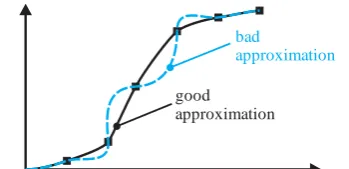
In order to design a neural network we also need to determine the number of neurons in the first layer. Common sense says that more neurons should be able to approximate functions better. There is however always a certain upper limit associated with this process. Too many neurons can namely also result in poor function approximation as demonstrated in Fig. 8.

Fig. 8: Good and poor function approximation



p1 p2 pR b1 w1,1 1

f

n1 a1

1

R 1x W

p

S Rx

b +

S 1x

f

n

S 1x S 1x

a R



b2 1

f

n2 a2



b1

wS,R

f

n1 a1

S

intralayer interlayer recurrent

feedforward feedback

1

R 1x W

1 p

S1x_R

b1 +

S 11 x

f

1

n1

S1 x₁

a1

R

S1x₁

1 W2 S S2x1

b2

+ n

_f

2 2

S2 x₁

S 12x

a2

S2x

1

1 W3 S S3x2

b3

+ n

_f

3 3

a3

S 13 x

S 13x

input first layer second layer third layer

1

R 1x W

1

p

S1x_R

b1

+

S 11x

n1

S1x₁

a1

R

S1x1

1

W2

S S2x 1

b2

+ n

2

S2x₁

S 12x

a2

S2x1

input logsig layer linear layer

good approximation

bad

[image:2.595.342.517.599.683.2] [image:2.595.51.293.604.694.2]

(3)

Its main application is function approximation. A very important question however still has to be answered. So far, nothing was said about the process of determining the correct values of the parameters w and b in order that the neural network functions properly. In order to do this a training process must be conducted. Although there is a myriad of training approaches, most of them fall in the following two categories [7]:

• Supervised learning

In this case a network is trained by a sequence of pairs of vectors. The first one is the input vector and the second one the target vector. The weights can be modified at each step (after each pair) or a matrix of all the vectors can be formed and then used for training. The training processes are therefore called incremental or batch learning [8].

• Unsupervised learning

In this case there are no target vectors. The weights are modified based only on the input vectors.

The algorithm used to train the two layer perceptron is the so called backpropagation algorithm (also known as Delta rule) [9]. It is composed of both forward and backward stage. It is described in some detail in [10]. The main goal of the algorithm is to make the difference between the actual and the target outputs as small as possible.

IV. PYTHON PROGRAM& RESULTS

In order to use Python, we must of course install it. On Windows platform it is very popular to install it together with Anaconda and then make the program in Jupyter Notebook [11]. Among many other possibilities a PyCharm software package canbe installed to use Python [12].

As already noted in the Introduction, Python is a high-level general-purpose programming language. It is especially popular among scientific community due to a wide set of freely available libraries, in particular scientific ones (linear algebra, visualization tools, plotting, image analysis, differential equations solving, symbolic computations, statistics etc.). Probably the three most important ones are Numpy, SciPy and Matplotlib [13]. NumPy is a library which adds a support for creation of large, multi-dimensional arrays and matrices, together with a large set of operations working on them [14].The SciPy software library implements a set of functions for processing scientific data, such as statistics, signal processing, image processing, and function optimization [15]. Matplotlib is, as the name of course suggests, a library used for plotting data [16]. Beside these common libraries, a Neurolab library, created specifically for neural networks implementation [17], will be used. The code starts with the import of the needed libraries:

importnumpy as np importneurolab as nl importpylab as pl

Then a two layer neural network is created by the following command:

net = nl.net.newff([[-10, 10]], [15, 1])

The parameters mean that the network expects inputs in the [-10, 10] range. The hidden layer has 15 neurons and the output layer 1 neuron. It should be emphasized that the weights are randomly initialized.

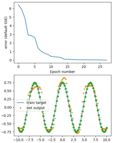
After that we need to create samples for neural network training. Let’s say that we want the neural network to approximate function 0.75 sin(s) in the range [-10, 10]. So, input vector x can be created by the following command:

x = np.linspace(-10, 10, 100)

It consists of 100 equally spaced values between -10 and 10. The corresponding output vector y can be easily obtained.

y = 0.75*np.cos(x)

In the next step we must reshape both x and y into column form. The len() function returns the number of items in an object.

size = len(x)

Then we can modify x and y into new vectors inp (input) and trg (target) by the following commands:

inp = x.reshape(size,1) trg = y.reshape(size,1)

The reshape() function’s arguments are the numbers of rows and columns in the new vector. Now, after the creation of the input and target vectors, we can train the neural network using them. We will use the following command:

error = net.train(inp, trg, epochs=300, show=100, goal=0.01)

The train() function we have used is the main part of the presented program. In order to get its detailed description, it is best to check the documentation [18]. It has several parameters. The first two are the input and the target vector. Then the number of epochs needs to be stated (the default value is 500). The show parameters determines the steps at which the error is printed out (the default value is 100). The goal parameter determines at which value of the error the training will stop (the default value is 0.01). It is also important to at least know which training algorithm is being used. The default is the “Gradient descent with momentum backpropagation and adaptive learning rate” algorithm (in Neurolab library it is known as neurolab.train.train_gdx(). Actually, all the default values can be obtained by the net.trainf.defaults command. The typical output of the program at this stage is given below:

Epoch: 100; Error: 0.02729823200135833; Epoch: 200; Error: 0.018311521643474635; Epoch: 300; Error: 0.01722912104269513;

The maximum number of train epochs is reached

(4)

during the network creation, we get a different result every time when we rerun the program. We might for example get the following output:

Epoch: 100; Error: 0.03487234318088822; Epoch: 200; Error: 0.01774028250123779; The goal of learning is reached

The error variable on the left side stores errors obtained during each training iteration. In order to comparethe actual output of the neural network with the target, we form the out

vector with the following command:

out = net.sim(inp)

So, in the out vector the actual values of the output of the neural network after training are stored. Now we just need to plot the results. We will lot the results in two subplots (one above the other). The first one will plot the error vector. We can get it with the following commands:

pl.subplot(211) pl.plot(error)

pl.xlabel('Epoch number') pl.ylabel('error (default SSE)')

The three digit parameter in the subplot() functions gives the number of rows, the number of columns and the index of the specific subplot. In order to visually analyze the performance of the neural network, we will compare the actual and the target output. This will be done in the second subplot using the following commands:

pl.subplot(212)

pl.plot(inp, trg, '-',inp , out, '.', inp, trg, 'p') pl.legend(['train target', 'net output']) pl.show()

[image:4.595.326.526.63.315.2]

The obtained output is shown in Fig. 9

Fig. 9: The result of the program

[image:4.595.332.520.388.625.2]

The result is by no means always that good. If for example we only use 20 values for training, we get the result shown in Fig. 10, despite the training goal being reached.

Fig 10: The result when only 20 values are used for training

[image:4.595.69.269.486.735.2]

When only 15 values are used, the result is even worse (see Fig. 11).

Fig 11: The result when only 15 values are used for training

(5)

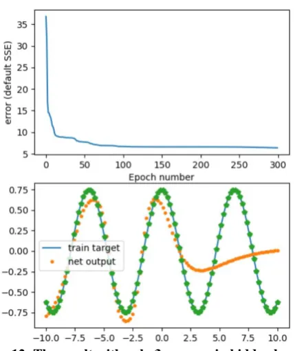
Fig 12: The result with only 3 neurons in hidden layer

[image:5.595.62.277.50.306.2]

Contrary to intuition, there is also a problem with neural network having too many neurons. If we discard longer training times needed when network has more neurons in hidden layer, a problem of overfitting might appear as well. If we use the network with 200 neurons in the hidden layer and then analyze with 500 values in the [-10,10] interval, we get the result shown in Fig. 13.

Fig. 13: The result with only 200 neurons in hidden layer

We can clearly see that many points are far from the target values, despite the goal of the training being reached.

V. CONCLUSION

Neural networks are still a hot topic within artificial intelligence field. In this paper a simple two layer perceptron used for function approximation is made in Python using Neurolab library. All the steps in the program are thoroughly explained. The performance of the network is also analyzed and the dependence of the network performance on the number of training samples and the number of neurons in the hidden layer are demonstrated. The whole procedure is valuable for anyone starting the study of neural networks and wanting them to be implemented in Python. The further step into more complex neural networks is facilitated in this way.

REFERENCES

1. L. V. Fausett, “Fundamentals of neural networks:

architectures, algorithms, and applications,” Prentice-Hall, 1994.

2. T. Lindblad, J. M. Kinser, and J. G. Taylor, J. G. “Image

processing using pulse-coupled neural networks,” Springer, 2005.

3. J. Howse, “OpenCV computer vision with Python,” Packt

Publishing, 2013.

4. J. L. McClelland, D. E. Rumelhart, and PDP Research Group,

“Parallel distributed processing,” Explorations in the Microstructure of Cognition, 2, 216-271, 1986

5. https://www.tiobe.com/tiobe-index/

6. R. Van Hattem, “Mastering Python,” Packt Publishing, 2016.

7. A. Zilouchian , and M. Jamshidi, “Intelligent control systems

using soft computing methodologies,” CRC press, 2001.

8. M. T. Hagan, H. B. Demuth, M. H. Beale, and O. De Jesus,

“Neural network design, 2nd Ed.,” Hagan and Demuth, 2013.

9. I. N. Da Silva, D. H. Spatti, D. H., R. A. Flauzino, R. A., L.

H. BartocciLiboni, and S. F. dos Reis Alves, “Artificial neural networks: A practical course,” Springer, 2017.

10. A. F. Gad, “Practical Computer Vision Applications Using

Deep Learning with CNNs,” Apress, 2018.

11. J. P. Mueller, “Beginning programming with Python for

dummies,” John Wiley & Sons, 2018.

12. Q. N. Islam, “Mastering PyCharm,” Packt Publishing, 2015.

13. R. Johansson, “Numerical Python: Scientific Computing and

Data Science Applications with Numpy, SciPy and Matplotlib, 2nd Ed.,” Apress, 2019.

14. I. Idris, “NumPy: Beginner's Guide, 3rd Ed.,” Packt

Publishing Ltd, 2015.

15. J. Nunez-Iglesias, S. van der Walt, and H. Dashnow, “Elegant

SciPy: The Art of Scientific Python," O'Reilly, 2017.

16. D. M. McGreggor, “Mastering matplotlib: A practical guide

that takes you beyond the basics of matplotlib and gives solutions to plot complex data,” Packt Publishing, 2015

17. https://pythonhosted.org/neurolab/

18. https://pythonhosted.org/neurolab/lib.html#neurolab.train.trai