https://doi.org/10.5194/angeo-36-1657-2018 © Author(s) 2018. This work is distributed under the Creative Commons Attribution 4.0 License.
Validation of Clyde River SuperDARN radar velocity measurements
with the RISR-C incoherent scatter radar
Alexander Koustov1, Robert Gillies2, and Peter Bankole1
1Department of Physics and Engineering Physics, University of Saskatchewan, Saskatoon, Saskatchewan, Canada 2Department of Physics and Astronomy, University of Calgary, Calgary, Alberta, Canada
Correspondence:Alexander Koustov ([email protected]) Received: 6 September 2018 – Discussion started: 14 September 2018 Accepted: 5 December 2018 – Published: 14 December 2018
Abstract. The study considers simultaneous plasma veloc-ity measurements in the eastward direction carried out by the Clyde River (CLY) Super Dual Auroral Radar Network (SuperDARN) high-frequency (HF) radar and Resolute Bay (RB) incoherent scatter radar – Canada (RISR-C). The HF velocities are found to be in reasonable agreement with RISR velocities up to magnitudes of 700–800 m s−1 while, for faster flows, the HF velocity magnitudes are noticeably smaller. The eastward plasma flow component inferred from SuperDARN convection maps (constructed for the area of joint measurements with consideration of velocity data from all the radars of the network) shows the effect of smaller HF velocities more notably. We show that the differences in eastward velocities between the two instruments can be sig-nificant and prolonged for observations of strongly sheared plasma flows.
1 Introduction
The Super Dual Auroral Radar Network (SuperDARN) high-frequency (HF) radars have been installed to continuously monitor the E×B plasma drift in the Earth’s ionosphere (Greenwald et al., 1995). To achieve this goal, the radars de-tect coherent ionospheric echoes from the F region and mea-sure their Doppler velocity. It is assumed that the decame-ter ionospheric irregularities, responsible for SuperDARN echoes, move with the velocity close to theE×B plasma drift. A number of comparisons of SuperDARN velocity measurements with concurrently operating incoherent scat-ter radars (ISRs) that measure the E×B plasma drift has been performed in the past (Ruohoniemi et al., 1987; Davies
et al., 1999, 2000; Milan et al., 1999; Xu et al., 2001; Gillies et al., 2009, 2010, 2018; Bahcivan et al., 2013; Koustov et al., 2016). These comparisons, overall, supported the above ma-jor assumption of the SuperDARN measurements. However, occasional significant differences between HF radar line-of-sight (LOS) velocities andE×Bdrift component along the beam have been noticed. Initially, these were thought to orig-inate from differences in the echo collecting areas and in the signal integration time (Davies et al., 1999) but the body of the data published so far questions this notion. It is now accepted that the HF velocities of the F region echoes are generally smaller (Gillies et al., 2018). One factor found to lead to this result is an assumption made during SuperDARN velocity measurements, which sets the index of refraction for the ionosphere of unity. However, this explanation can-not account for large differences of more than 20 %–30 %. Koustov et al. (2016) stressed the original finding by Xu et al. (2001) that the HF velocity magnitudes are substantially smaller (up to a factor of 2) than theE×Bdrift component for high-speed flows exceeding 1000 m s−1. Furthermore, the HF velocity magnitudes are often larger than theE×Bflow component along the radar beam (e.g., Ruohoniemi et al., 1987; Koustov et al., 2016; Gillies et al., 2018). Such obser-vations have been interpreted in terms of lateral deviation of HF radar beams (Koustov et al., 2016; Gillies et al., 2018). Other SuperDARN–ISR velocity inconsistencies have been associated with the occurrence of E region echoes at tradi-tionally expected F region ranges for SuperDARN (Bahcivan et al., 2013; Gillies et al., 2018).
con-this effort complements the previous validation work for the Rankin Inlet (RKN) and Inuvik (INV) SuperDARN radars by Koustov et al. (2009), Mori et al. (2012), Bahcivan et al. (2013), Koustov et al. (2016), and Gillies et al. (2018). Since the CLY radar currently provides a significant contri-bution to the global-scale convection mapping with Super-DARN such work is of particular importance. We take advan-tage of the availability ofE×Bplasma drift measurements made by the recently installed Resolute Bay (RB) incoherent scatter radar – Canada (RISR-C) (e.g., Gillies et al., 2016). In the present work, we compare CLY- and ISR-based velocities in a different way than the previous studies.
Traditionally, gate-by-gate comparison of data from two radar systems that make measurements in roughly the same directions is performed (e.g., Gillies et al., 2018). Such an ap-proach cannot be implemented for the CLY–RISR-C geom-etry because none of these radar’s beams are close enough in terms of their direction (see map on Fig. 1 in Gillies et al., 2018). For this reason, we consider RISR-C two-dimensional vectors in a certain area (which are inferred by merging data from multiple individual beams using the ap-proach by Heinselman and Nicolls, 2008) and compare them with CLY data averaged over three beams and four gates. Thus, we assess the data in a statistical sense, in terms of the average and median velocities over a large spatial domain.
A validation using highly averaged data is appropriate since the SuperDARN global-scale maps of plasma flow obtained with the Potential Fit technique (Ruohoniemi and Baker, 1998; Shepherd and Ruohoniemi, 2000) are built us-ing median-filtered line-of-sight (LOS) velocities (the so-called gridded velocities). These are inferred from up to 27 LOS velocity values in bins consisting of data in neighboring range gates (one smaller number gate and one larger number gate) and radar beams (one smaller number beam and one larger number beam) and for three consecutive radar scans. This implies that the input to the Potential Fit procedure is a highly smoothed HF velocity covering 3–6 min of raw data and a significant space domain. In this view, there is a sense in considering 2-D RISR-C data and comparing them with HF velocity medians, or vectors from the convection maps, over large spatial areas of overlap.
Although our aim is to validate the CLY velocity measure-ments, there is additional value from the CLY–RISR compar-ison. The RISR method of velocity vector estimations also has some limitations (Heinselman and Nicolls, 2008) that need testing. A couple of the limitations we will consider are a lack of velocity measurements along magnetic field lines and the expectation of spatially quasi-uniformity of flows,
2 Geometry of RISR-C and Clyde River radar observations
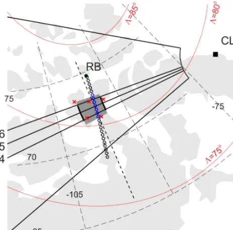
Figure 1 shows the fields of view (FoVs) of the CLY and RKN SuperDARN radars starting from range gate 5 and the location of the RB incoherent scatter radar RISR-C, which we will simply refer to as the RISR radar hereafter. This radar makes measurements in multiple beams; it uses 11 beams in the called “world-day” mode and 51 beams in the so-called “imaging” mode. Measured line-of-sight velocities in all the beams and at all ranges are used to infer 2-D vectors of theE×B plasma flow according to the procedure out-lined by Heinselman and Nicolls (2008). The resultant vec-tors are reported with 0.25◦bin size of magnetic/geographic latitude. The points to which the measurements are assigned are shown in Fig. 1 for the height of 300 km. The actual cen-terline for the points of data merging depends on data avail-ability in specific beams (Gillies et al., 2018).
Figure 1 also shows the orientation of the CLY beams 4, 5, 6 (along their centers), and the area from which data were considered, the shaded rectangle region flanked by beams 4 and 6 between range gates 18 and 22. The monitored iono-spheric region is centered at geographic latitude of∼72.5◦. An important feature of this area is that within these range gates the CLY beams 4–6 are almost parallel to the lines of equal geographic latitude at the chosen radar range gates, as shown in Fig. 1. This means that one can directly compare CLY LOS velocities with the eastward component (in geo-graphic coordinates) of a RISRE×B velocity vector. We note that the area of CLY observations was also covered by measurements from the RKN and INV radars (and occasion-ally by the Saskatoon and Kodiak SuperDARN radars), so that SuperDARN convection maps were usually well con-strained.
3 Methodology of the LOS velocity comparison
Figure 1.Field of view of the SuperDARN radar at CLY. The black straight lines are the orientation of specific beams (4–6) that were considered in this study. Shaded areas represent areas of HF radar data averaging. RB is the location of the RISR-C ISR. The radar reports theE×Bvector with a bin size of 0.25◦of geographic lat-itude for points shown as black circles stretching roughly along the magnetic meridian crossing the RB zenith. The blue-colored circles are those locations whose data were used for comparison with the CLY measurements. The solid red arcs are the magnetic latitudes of 75, 80, and 85◦.
Our approach to the CLY–RISR velocity comparison is as follows. We first select a 5 min period of RISR velocity mea-surements at geographic latitudes of∼71.625–73.125◦(see blue circles in Fig. 1) and compute the median velocity value for RISR. We then compute the median value of the CLY ve-locity over matching 5 min interval in three beams and four gates, as mentioned above. The matched data pair is then en-tered into a common data set.
[image:3.612.52.284.67.296.2]Figure 2 shows the total number of 5 min intervals of joint RISR–CLY radar measurements, times when RISR and CLY both made measurements in the blue and shaded regions shown in Fig. 1, as a function of UT. This histogram distribu-tion does not include individual events when CLY data were obviously contaminated by ground scatter profoundly affect-ing the velocity comparison (Gillies et al., 2018). The ground scatter was identified with the conventional selection criteria (e.g., Sect. 4.1 in Ponomarenko et al., 2007). The number of intervals was much larger from noon to dusk (local solar noon is at about 19:00 UT).This is because of the preferen-tial occurrence of CLY echoes at ranges of interest during the daytime (Ghezelbash et al., 2014).
Figure 2.Number of CLY–RISR 5 min intervals of joint observa-tions for all data considered. Total number of available intervals is shown in the top-left corner. For the area of observations, local time (scale at the top) roughly coincides with the magnetic local time.
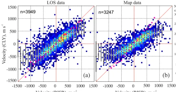
4 Results for CLY LOS velocity and RISR comparison Figure 3a shows the CLY LOS velocity versus the RISR east-wardE×Bcomponent for the entire data set, produced as described above. The total number of points is close to 4000, which is a significant number. Overall, both positive and neg-ative velocities are well represented. Although some spread is present, a significant amount of points are located close to the line of equality. To assess the plot, we binned the data ac-cording to the RISR measurements by using 100 m s−1bins of the latter. Binned in this way CLY velocity medians are shown by black–white dots. The vertical black–white bars crossing each dot are the binned CLY velocity value±1 stan-dard deviation. We also binned the data of Fig. 3 according to bins of the CLY velocity (pink asterisks, shown by thin symbols in order to not contaminate the plot).
The black–white dots are reasonably close to the line of the perfect agreement.The pink asterisks are actually very close to the line of equality. Good alignment with the line of equality and good correspondence between the location of the black dots and pink asterisks indicate that the veloci-ties are almost linearly related, especially in the range from −500 to +500 m s−1. One clear departure of the back dots from the line of equality are the RISR velocities with magni-tudes greater than∼750 m s−1.
An alternative way of assessing the data trends in Fig. 3a is to make a linear fit to the cloud of points. Parameters of the linear fit are presented in Table 1 for four ranges of the RISR velocity,±500,±750,±1000, and±1500 m s−1. The slope is 0.73 for the smallest velocities of±500 m s−1, which in-cludes about 71 % of all the data points. A linear fit to almost all the data has a decreased slope of 0.64.
5 Methodology of vector comparison between SuperDARN and RISR
Figure 3. (a)Scatterplot of the CLY LOS velocity versusE×Beastward velocity component as inferred by RISR. Total number of pointsn is shown in the top-left corner. The black–white dots are medians of the CLY velocity in 100 m s−1bins of RISR velocity. The black vertical lines are the standard deviations of the CLY velocity in each bin. The pink dots are medians of the RISR velocity in 100 m s−1bins of CLY measurements.(b)The same as(a)but the eastward flow component inferred from SuperDARN flow maps was considered.
Table 1.Parameters of the linear fit line VelocityCLY=a·VelocityRISR+b, the number of points involved in the fitting, and the squared
correlation coefficient for various ranges of the RISR velocity. Left three columns are the LOS velocity comparison while right three columns are for the 2-D velocity comparison.
LOS comparison 2-D comparison
m s−1 a b(m s−1) Points R2 a b(m s−1) Points R2 ±500 0.73 −9.90 2815 0.46 0.59 −16.32 2202 0.45
±750 0.71 −10.29 3558 0.58 0.56 −11.31 2851 0.57 ±1000 0.68 −8.27 3823 0.6 0.54 −9.91 3106 0.62
±1500 0.64 −5.31 3932 0.6 0.502 −7.08 3227 0.61
consideration to the same area of joint CLY–RISR obser-vations as in the LOS comparison, shown in Fig. 1. Here the SuperDARN convection vectors are available at geo-magnetic latitudes of 80.5–81.5◦and∼7◦of magnetic lon-gitude. In this area, the convection maps and vectors are mostly based on RKN, INV, and CLY radar measurements with only occasional contributions from other SuperDARN radars. We selected the three grid nodes at 81.5◦ magnetic latitude (MLAT) that were closest to the area of the CLY LOS velocity assessment and the two closest grid nodes at 80.5◦ magnetic latitude, marked by red crosses in Fig. 1. For each vector location, the geographic east component of the flow was computed and the median value (out of poten-tially five values, although for some periods it was as low as one measurement) was calculated to represent the eastward plasma flow component of a 5 min SuperDARN map. This is not a traditional temporal resolution for the SuperDARN mapping (which is usually 2 min); such data processing has been done to avoid the need of additional averaging of 2 min SuperDARN maps. Unfortunately, the start times of RISR measurement intervals were often irregularly spaced while SuperDARN maps were synchronized to exactly correspond
to 5 min boundaries (i.e., 0–5, 10–15 min, etc.). For the com-parison, only HF and ISR data that were less than 2 min apart were considered. For this reason, even when both radar sys-tems were operational, the actual number of joint points per hour was below the expected number of 12.
[image:4.612.141.454.342.425.2]6 Results for vector comparison between SuperDARN and RISR
Figure 3b plots the eastward component of the plasma flow measured by RISR and SuperDARN. The spread of the data looks similar to that of Fig. 3a (the LOS comparison). We assessed Fig. 3b using the same methods as performed on Fig. 3a (see Sect. 4). Overall agreement of the data clearly holds.
Several results from Fig. 3b are consistent with the data of Fig. 3a. First, the SuperDARN map-based velocities are somewhat smaller than those of RISR. This is recogniz-able through an obvious deviation of the distribution max-ima from the line of equality, especially at RISR positive ve-locities of > 500 m s−1. Secondly, the tendency for the Su-perDARN velocity being smaller is greater for larger RISR magnitudes. This feature is seen for both positive and nega-tive RISR velocities. Finally, consistent with previous reports (Koustov et al., 2016; Gillies et al., 2018), there is a number of points for which the radars show oppositely directed flows. This was more frequent for small RISR velocities. Although Fig. 3 shows good consistency of the data provided by the two radar systems, the differences can be as large as a factor of 2 in individual measurements.
The agreement between the convection vectors given by RISR and SuperDARN is expected. We see that the consis-tency deteriorates once 2-D data are involved, but mostly at intermediate velocity magnitudes of 300–600 m s−1. The
in-consistencies are characterized by slower SuperDARN ve-locities. Interestingly, the differences for large velocity mag-nitudes in Fig. 3b are comparable to those in Fig. 3a.
To assess the data trends in Fig. 3b in an alternative way, linear fits to the scatter of points in Fig. 3b were made for four ranges of the RISR velocity of±500,±750,±1000, and ±1500 m s−1, similar to those for the LOS velocity compar-ison. The slope of the fitted line, theyintercept, the number of points involved in each fitting, and the squared correla-tion coefficient are presented in Table 1. The slopes are close to 0.6 for the set of smallest velocities (±500 m s−1), which includes about 68 % of all the available data. The slope de-creases to 0.5 if almost all the data are considered. We think that the deterioration of the agreement at intermediate and large velocity magnitudes is due to the broader area over which the SuperDARN data are averaged for the 2-D com-parison. In this case, there is more chance for SuperDARN to include ground-scatter-contaminated measurements, giv-ing effectively slower grid velocities to the fittgiv-ing procedure.
7 On possible reasons for velocity disagreements One reason frequently given for the systematic underesti-mation of the SuperDARN velocity measurements is the as-sumption that the index of refraction is unity (Gillies et al., 2009; Ponomarenko et al., 2009). We attempted to evaluate
the importance of this effect in our data set. A plot similar to Fig. 3a was produced, but with the CLY velocity being corrected by considering the electron density (at the F region peak) measured by RISR. The plot looked very much similar to Fig. 3a. We assessed the plot by applying the linear fit line to the HF velocity medians in 100 m s−1bins of RISR veloc-ity, considering the range of almost linear dependence, be-tween−1000 and+1000 m s−1of RISR velocities. The slope of the best fit line improved to∼0.75 (from∼0.65). This improvement is consistent with the previous studies though it does not entirely account for the differences between the radar measurements.
We also investigated the diurnal variation of the veloc-ity ratioR=VelHF/VelRISR as done previously by Gillies
et al. (2018) to explore possible influences of the refrac-tive index on velocity using typical local time variations in the electron density as a proxy for refractive index. For the winter and equinoctial ionosphere over Resolute Bay, the largest densities are systematically observed near local solar noon and during the afternoon hours (18:00–22:00 UT) (e.g., Ghezelbash et al., 2014; Themens et al., 2017). It is therefore expected that the velocity ratioR would be smallest during these times, as reported by Gillies et al. (2018) for the RKN radar. The nighttime results by Gillies et al. (2018) are more confusing. First, strangely, the ratios here were often above 1 at latitudes southward of RB and systematically below 1 (but not as far below unity as they were near noon) at lati-tudes poleward of RB. Gillies et al. (2018) indicated that the vertical plasma flow velocities in RISR measurements were, very likely, incorrectly estimated for nighttime observations. Since the observation area in our comparison is close to RB, we expect that this effect will also affect the RISR–CLY com-parison.
Figure 4 plots the hourly median ratioRas a function of time for our CLY–RISR data set. One can see thatR varies significantly. It is lower during daytime (noon is at about 19:00 UT) than during dawn/prenoon (12:00–18:00 UT), but its values are smallest during nighttime (midnight is at about 07:00 UT). Interestingly, the average ratio over all UTs is 0.83, which is closer to 1 than the slopes of the lines in Fig. 3 (Table 1). This is probably because the infrequent high-velocity data are averaged out by dominating data at low velocities in certain RISR bins of Fig. 4.
Figure 4.Line plot of the hourly median velocity ratioRversus UT for the CLY radar. The data set is the same as for Fig. 3a. For the area of observations, local time (scale at the top) roughly coincides with the magnetic local time.
Gillies et al. (2018) believe that large nighttime ratios of RKN to RISR velocity could be due to errors in HF measure-ments because the RKN beams can experience significant lateral deviations so that actual measurements are performed at smaller flow angles with a larger LOS velocity compo-nent. This explanation cannot be applied to our observations. This is because the CLY radar observes azimuthally, along the average plasma flow most of the time (except of short periods at near noon and near midnight when the flows are predominantly meridional) so that lateral deviations of the CLY beams would lead to, depending of the orientation of the plasma flow with respect to the CLY beam, either smaller or larger LOS velocities.
[image:6.612.48.288.65.187.2]We think that the HF–RISR velocity inconsistency can also originate, at least partially, from the nature of HF signal formation. The effect has been discussed in general terms by Uspensky et al. (1989) as applied to E region coherent scatter and by Koustov et al. (2016) for F region coherent backscatter. The flows in the nighttime ionosphere are very likely to be more patchy/grainy with occasional occurrence of regions with enhanced flow magnitude (low electron den-sity) and decreased flow magnitude (high electron denden-sity). We argue that in the case of a patchy ionosphere there is a good chance that the ratio R would be smaller than in the case of a uniform ionosphere and homogeneous flow. Flow enhancements and decreases affect both RISR and HF mea-surements but in a profoundly different manner. The RISR radar would average the velocity in patches with enhanced and depleted electron density together, and it would report what can be classified as the background flow velocity. In the presence of electron density patches with enhanced and de-creasedE×Bplasma flows, HF radars would preferentially detect stronger signals from those areas where the electron density is enhanced, and the electric field (flow magnitude) is decreased, so that they would show somewhat smaller ve-locity than the background value measured by an incoherent scatter radar.
Figure 5.Eastward component of theE×Bdrift as measured by RISR (diamonds, 5 min resolution data) and matched velocity me-dians of CLY observations (blue circles, 5 min meme-dians of original 1 min measurements in beams and gates overlapping the region of RISR observations) for the event of 4 March 2016. For the area of observations, local time (scale at the top) roughly coincides with the magnetic local time.
It is conceivable to have the opposite situation with HF ve-locities above the background flow if regions with enhanced density have a stronger local electric field, as discussed in Uspensky et al. (1989). In this respect, Koustov et al. (2016) and Gillies et al. (2018) noticed that HF velocities could be larger than theE×B plasma drift component measured by ISRs. Such points are occasionally seen in previously pub-lished data (Ruohoniemi et al., 1987; Davies et al., 1999). Our data in Fig. 3 also show such points but, in general, the data agree fairly well. Although the work of Koustov et al. (2016) and Gillies et al. (2018) related the larger HF ve-locity effect to lateral deviations of the HF radar beams from the expected directions, it could partially be due to the afore-mentioned effect of ionospheric microstructuring.
Potentially, lowR values can be related to the occurrence of misidentified ionospheric scatter because some iono-spheric echoes with low velocities can actually be ground or mixed ionospheric and ground scatter. Gillies et al. (2018) showed that removal of points that could potentially be af-fected by ground scatter improves the RKN–RISR veloc-ity agreement significantly. Our analysis showed that ground scatter is rare during winter and equinox nighttime for the CLY radar, which is consistent with low nighttime F region densities (Ghezelbash et al., 2014; Themens et al., 2017). We also have to remind the reader that presumably obvious events with CLY ground-scatter contamination have been re-moved from our consideration in Fig. 3.
velocities differ consistently by several hundred m s−1over a period of almost 2 h.
Figure 6a illustrates the typical spatial velocity distribu-tion within the radar FoV, for one velocity scan during the above event. A sharp change in the LOS velocity polarity in the poleward and equatorward portions of the FoV is notice-able. The polarity transition occurs in the central beams 5–7. Figure 6b gives a global-scale map of plasma flow inferred from all SuperDARN radar measurements. The flow pattern in Fig. 6b was calculated by applying the new SuperDARN statistical model by Thomas and Shepherd (2018) which be-came available just recently. The map has a number of vec-tors originating from the RKN and INV radar measurements as well as those from CLY measurements. The presence of highly curved flows is evident near noon. Under these con-ditions, both SuperDARN and RISR can have difficulties in the construction of a 2-D vector field.
We comment that the flows seen in Fig. 6 are sunward, roughly along the magnetic meridian near noon, signifying the occurrence of a reverse convection cell. This is expected since the IMF Bz was steady at about+4 nT starting from 18:30 UT all the way until∼22:00 UT for this event.
Evaluating the extent to which the SuperDARN and RISR vectors are affected by the shear in the flow is difficult. We can see that the centers (foci) of the convection cells, accord-ing to RISR and SuperDARN, do not coincide in latitude for many maps in this event. In addition, the agreement between the RISR and SuperDARN map data improves dramatically when only the lower latitude SuperDARN map data are con-sidered.
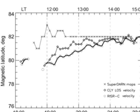
We investigated this further by determining the location of the convection reversal boundary (CRB) for the reverse vection cell (like that shown in Fig. 6b by the dashed con-tour). This is done by considering the standard 2 min Super-DARN maps, the CLY LOS velocity maps, and by looking at the reversal in the latitudinal profile of the RISR velocity (these are given for 5 min intervals). The CRB location based on the SuperDARN maps was determined by finding the mid-dle latitude between the two neighboring points on a standard plasma flow map with opposite directions of the flow, toward the Sun and away from the Sun. The CRB location based on the CLY LOS velocity maps was determined by plotting the LOS velocity versus beam number and finding the az-imuth and the range of the point at which the LOS veloc-ity is zero. The CRB location from the RISR measurements was found by plotting the azimuthal component of the RISR plasma flow versus latitude and finding the latitude with zero velocity. All the CRB locations were given in terms of the ge-omagnetic latitude. The accuracy of the CRB determination in all cases is on the order of half of a degree of geomagnetic latitude.
The resulting data are presented in Fig. 7. The CRB in-ferred from SuperDARN maps is located almost 2◦higher in MLAT than that determined from both CLY velocity maps and RISR data at the beginning of the event, and the
differ-ences are minimal toward the end of the event. The fact that the CRB location from CLY velocity maps is closer to that inferred from RISR data hints that perhaps the SuperDARN fitting procedure is the major factor for strong differences be-tween the SuperDARN maps and RISR measurements in this specific event. This is not to say that RISR measurements are exact; they are very likely also subject to errors under these strongly sheared and curved flows. One reason could be that the solution for the 2-D velocity vector field from the origi-nal LOS RISR data (Heinselman and Nicolls, 2008) smooths out the true sharp changes of the flow. Having a wider FoV for the RISR radar is expected to improve the quality of the flow pattern derivation under such conditions.
8 Summary and conclusions
In this study, we attempted to validate the CLY SuperDARN radar velocity measurements by comparing them with the data collected by the Resolute Bay incoherent scatter radar. Because no line-of-sight velocity comparison is possible for the geometry of joint observations, we adopted here a differ-ent approach. Namely, we considered the eastward compo-nent of theE×Bflow vector, as inferred from RISR mea-surements in multiple beams, and compared it to CLY ve-locities from a number of eastward-oriented beams and with the eastward component of the plasma flow inferred from 2-D Super2-DARN maps. The analysis undertaken allows us to draw several conclusions.
The CLY radar velocities measured in beams 4–6 are sta-tistically comparable to theE×Bcomponent of the plasma drift along these beams (eastward/azimuthal plasma flows) as measured by the RISR incoherent scatter radar. This implies that the velocity data provided by the CLY radar to the Su-perDARN database are reliable and suitable for convection mapping involving all SuperDARN radars. The comparisons performed are an addition to the previous validation work for the RKN and INV SuperDARN radars.
The slope of the best linear fit line to the CLY velocity variation versusE×B component (as measured by RISR) applied to the binned values is on the order of 0.65 if all the available data (removing data with obvious ground-scatter contamination) in the range±1000 m s−1are consid-ered. Correction of HF velocities on the index-of-refraction effect improves the slope to∼0.75. The slope of the linear fit line for the corrected data is still below 1, implying that additional factors affect the relationship. Additionally, diur-nal variations of the ratio of HF velocity to the RISR velocity show their strongest decrease below 1 during nighttime but not daytime. This implies that the deterioration of the RISR– SuperDARN velocity agreement at nighttime is caused not by the index-of-refraction effect but by other factors.
Figure 6. (a)A CLY LOS velocity map at 19:55 UT on 4 March 2016 and(b)a 5 min convection map calculated from all SuperDARN radar measurements for the same period of time. The TS2018 statistical model (Thomas and Shepherd, 2018) of order 8 for the solar wind electric field of 2.1 mV m−1was used. Contours of the electric potential are 6 kV apart.
Figure 7.Magnetic latitude of the flow reversal location within the dayside reverse convection cell as inferred from SuperDARN con-vection maps (crosses), CLY LOS velocity maps (diamonds), and RISR measurements for the event of 4 March 2016. For the area of observations, local time (scale at the top) roughly coincides with the magnetic local time.
One factor that may contribute to slower HF velocities, in addition to the refractive index, is the nature of HF signal col-lection. HF radars receive stronger signals from ionospheric regions with enhanced electron density where the electric field and/orE×Bplasma drift can be decreased compared to the background plasma.
In the case of highly sheared plasma flows, such as near dayside reverse convection cells occurring under strongly
dominant IMFBz>0, the differences between RISR and Su-perDARN velocity vectors can be large.
The reasonable agreement between the velocities of the two systems quantified as the slopes of the linear fit lines at the level of 0.6–0.8 for both the LOS and 2-D compar-isons implies that the RISR technique of theE×B deriva-tion from multiple individual radar beams is usually a reliable method most of the time. The comparison suggests that the RISR vectors are less reliable in the midnight sector where the flows are often very irregular, and strong vertical motions occur.
Data availability. SuperDARN data can be obtained from https: //superdarn.ca (last access: 11 December 2018). RISR-C data are available at http://data.phys.ucalgary.ca (last access: 11 Decem-ber 2018).
Author contributions. RG and PB worked on raw data processing and their preliminary analysis. PB prepared some diagrams. AK did most of the comparison work and wrote the initial manuscript. All authors participated in the writing, and all commented on the paper.
Competing interests. The authors declare that they have no conflict of interest.
[image:8.612.50.286.319.508.2]Canadian Foundation for Innovation, Canadian Space Agency’s Geospace Observatory (GO Canada) continuation initiative to the University of Saskatchewan radar group, and NSERC Discovery grant to Alexander Koustov. The University of Calgary RISR-C radar is funded by the Canada Foundation for Innovation and is a partnership with the US National Science Foundation and SRI International. We thank C. Graf for the initial analysis of RISR density data and R. Fiori for the help in software development. Dis-cussions of various aspects of the paper with Pavlo Ponomarenko and his help in software development are appreciated. The authors are indebted to two anonymous reviewers who not only identified weaknesses in the original manuscript but also made numerous constructive suggestions and, in addition, tremendously improved the writing style.
Edited by: Steve Milan
Reviewed by: two anonymous referees
References
Bahcivan, H., Nicolls, M. J., and Perry, G.: Comparison of Super-DARN irregularity drift measurements and F-region ion veloci-ties from Resolute Bay ISR, J. Atmos. Sol.-Terr. Phy., 105–106, 325–331, https://doi.org/10.1016/j.jastp.2013.02.002, 2013. Bristow, W. A., Hampton, D. L., and Otto, A.:
High-spatial-resolution velocity measurements derived us-ing Local Divergence-Free Fitting of SuperDARN ob-servations, J. Geophys. Res.-Space, 121, 1349–1361, https://doi.org/10.1002/2015JA021862, 2016.
Davies, J. A., Lester, M., Milan, S. E., and Yeoman, T. K.: A com-parison of velocity measurements from the CUTLASS Finland radar and the EISCAT UHF system, Ann. Geophys., 17, 892– 902, https://doi.org/10.1007/s00585-999-0892-9, 1999. Davies, J. A., Yeoman, T. K., Lester, M., and Milan, S. E.:Letter to
the Editor:A comparison of F-region ion velocity observations from the EISCAT Svalbard and VHF radars with irregularity drift velocity measurements from the CUTLASS Finland HF radar, Ann. Geophys., 18, 589–594, https://doi.org/10.1007/s00585-000-0589-6, 2000.
Ghezelbash, M., Koustov, A. V., Themens, D. R., and Jay-achandran, P. T.: Seasonal and diurnal variations of Po-larDARN F region echo occurrence in the polar cap and their causes, J. Geophys. Res.-Space, 119, 10426–10439, https://doi.org/10.1002/2014JA020726, 2014.
Gillies, R. G., Hussey, G. C., Sofko, J. G., McWilliams, K. A., Fiori, R. A. D., Ponomarenko, P. V., and St.-Maurice, J.-P.: Improvement of SuperDARN velocity measurements by estimating the index of refraction in the scattering re-gion using interferometry, J. Geophys. Res., 114, A07305, https://doi.org/10.1029/2008JA013967, 2009.
Gillies, R. G., Hussey, G. C., Sofko, G. J., Wright, D. M., and Davies, J. A.: A comparison of EISCAT and SuperDARN F-region measurements with consideration of the refractive in-dex in the scattering volume, J. Geophys. Res., 115, A06319, https://doi.org/10.1029/2009JA014694, 2010.
Gillies, R. G., van Eyken, A., Spanswick, E., Nicolls, M. J., Kelly, J., Greffen, M., Knudsen, D., Connors, M., Schutser, M., Valentic, T., Malone, M., Buonocore, J., St.-Maurice,
J.-P., and Donovan, E.: First observations from the RISR-C incoherent scatter radar, Radio Sci., 51, 1645–1659, https://doi.org/10.1002/2016RS006062, 2016.
Gillies, R. G., Perry, G. W., Koustov, A. V., Varney, R. H., Reimer, A. S., Spanswick, E., St.-Maurice, J.-P., and Donovan, E.: Large-scale comparison of polar cap ionospheric velocities, measured by RISR-C, RISR-N, and SuperDARN, Radio Sci., 53, 624–639, https://doi.org/10.1029/2017RS006435, 2018.
Greenwald, R. A., Baker, K. B., Dudeney, J. R., Pinnock, M., Jones, T. B., Thomas, E. C., Villain, J.-P., Cerisier, J.-C., Senior, C., Hanuise, C., Hunsuker, R. D., Sofko, J. G., Koehler, J. A., Nielsen, E., Pellinen, R., Walker, A. D. M., Sato, N., and Ya-magishi, H.: DARN/SuperDARN: A global view of the dynam-ics of high-latitude convection, Space Sci. Rev., 71, 761–796, https://doi.org/10.1007/BF00751350, 1995.
Heinselman, C. J. and Nicolls, M. J.: A Bayesian approach to elec-tric field and E-region neutral wind estimation with the Poker Flat Advanced Modular Incoherent Scatter Radar, Radio Sci., 43, RS5013, https://doi.org/10.1029/2007RS003805, 2008. Koustov, A. V., St-Maurice, J.-P., Sofko, G. J., Andre, D.,
Mc-Dougall, J. W., Hairston, M. R., Fiori, R. A., and Kadochnikov, G. E.: Three-way validation of the Rankin Inlet Polar-DARN radar velocity measurements, Radio Sci., 44, RS4003, https://doi.org/10.1029/2008RS004045, 2009.
Koustov, A. V., Lavoie, D. B., and Varney, R. H.: On the consistency of the SuperDARN radar velocity andE×Bplasma drift, Ra-dio Sci., 51, 1792–1805, https://doi.org/10.1002/2016RS006134, 2016.
Milan, S. E., Davies, J. A., and Lester, M.: Coherent HF radar backscatter characteristics associated with auroral forms identi-fied by incoherent radar techniques: A comparison of CUTLASS and EISCAT observations, J. Geophys. Res., 104, 22591–22604, https://doi.org/10.1029/1999JA900277, 1999.
Mori, D., Koustov, A. V., Jayachandran, P. T., and Nishitani, N.: Resolute Bay CADI ionosonde drifts, PolarDARN HF veloci-ties and SuperDARN cross polar cap potential, Radio Sci., 47, RS3003, https://doi.org/10.1029/2011RS004947, 2012. Ponomarenko, P. V., Waters, C. L., and Menk, F. W.: Factors
deter-mining spectral width of HF echoes from high latitudes, Ann. Geophys., 25, 675–687, https://doi.org/10.5194/angeo-25-675-2007, 2007.
Ponomarenko, P. V., St-Maurice, J.-P., Waters, C. L., Gillies, R. G., and Koustov, A. V.: Refractive index effects on the scat-ter volume location and Doppler velocity estimates of iono-spheric HF backscatter echoes, Ann. Geophys., 27, 4207–4219, https://doi.org/10.5194/angeo-27-4207-2009, 2009.
Ruohoniemi, J. M. and Baker, K. B.: Large-scale imaging of high-latitude convection with Super Dual Auroral Radar Network HF radar observations, J. Geophys. Res., 103, 20797–20811, https://doi.org/10.1029/98JA01288, 1998.
Ruohoniemi, J. M., Greenwald, R. A., Baker, K. B., Villain, J.-P., and McCready, M. A.: Drift motions of small-scale irregulari-ties in the high-latitude F region: An experimental comparison with plasma drift motions, J. Geophys. Res., 92, 4553–4564, https://doi.org/10.1029/JA092iA05p04553, 1987.
Thomas, E. G. and Shepherd, S. G.: Statistical patterns of ionospheric convection derived from mid-latitude, high-latitude, and polar SuperDARN HF radar obser-vations, J. Geophys. Res.: Space Physics, 123, 3196– 3216 https://doi.org/10.1002/2018JA025280, 2018.