Ab initio multiple cloning algorithm for quantum nonadiabatic molecular dynamics.

This is a repository copy of Ab initio multiple cloning algorithm for quantum nonadiabatic molecular dynamics..

White Rose Research Online URL for this paper: http://eprints.whiterose.ac.uk/88795/

Version: Accepted Version

Article:

Makhov, DV, Glover, WJ, Martinez, TJ et al. (1 more author) (2014) Ab initio multiple cloning algorithm for quantum nonadiabatic molecular dynamics. Journal of Chemical Physics, 141 (5). 054110. ISSN 0021-9606

https://doi.org/10.1063/1.4891530

Reuse

Items deposited in White Rose Research Online are protected by copyright, with all rights reserved unless indicated otherwise. They may be downloaded and/or printed for private study, or other acts as permitted by national copyright laws. The publisher or other rights holders may allow further reproduction and re-use of the full text version. This is indicated by the licence information on the White Rose Research Online record for the item.

Takedown

If you consider content in White Rose Research Online to be in breach of UK law, please notify us by

Ab initio

_{Multiple Cloning algorithm for quantum nonadiabatic}

molecular dynamics

Dmitry Makhov,1William J. Glover,2,3Todd J. Martinez,2,3Dmitrii Shalashilin1

1

Department of Chemistry, University of Leeds

2

Department of Chemistry and The PULSE Institute, Stanford University, Stanford, CA 94305

3

SLAC National Accelerator Laboratory, Menlo Park, CA

Abstract: We present a new algorithm forab initio quantum nonadiabatic molecular dynamics

that combines the best features ofab initio Multiple Spawning (AIMS) and Multiconfigurational

Ehrenfest (MCE) methods. In this new method,ab initiomultiple cloning (AIMC), the individual

trajectory basis functions (TBFs) follow Ehrenfest equations of motion (as in MCE). However,

the basis set is expanded (as in AIMS) when these TBFs become sufficiently mixed, preventing

prolonged evolution on an averaged potential energy surface. We refer to the expansion of the

basis set as “cloning,” in analogy to the “spawning” procedure in AIMS. This synthesis of AIMS

and MCE allows us to leverage the benefits of mean-field evolution during periods of strong

nonadiabatic coupling while simultaneously avoiding mean-field artifacts in Ehrenfest dynamics.

We explore the use of time-displaced basis sets, “trains,” as a means of expanding the basis set

for little cost. We also introduce a new bra-ket averaged Taylor expansion (BAT) to approximate

the necessary potential energy and nonadiabatic coupling matrix elements. The BAT

approximation avoids the necessity of computing electronic structure information at intermediate

points between TBFs, as is usually done in saddle-point approximations used in AIMS. The

efficiency of AIMC is demonstrated on the nonradiative decay of the first excited state of

ethylene. The AIMC method has been implemented within the AIMS-MOLPRO package, which

I. Introduction

The dynamics of electronically nonadiabatic transitions is fundamental to many

photoinduced processes in chemistry and biochemistry. Examples include photosynthetic light

harvesting, the first events in visual reception in rhodopsin, and fluorescent sensors such as the

Green Fluorescent Protein (GFP). As the dynamical events in these problems are initiated by

electronic excitation, multiple electronic states and nonadiabatic transitions between these states

are invariably involved. Furthermore, both nuclear and electronic coherence effects can be

crucial, as recently shown in the context of photosynthetic light harvesting.1-5 An acceptable

model for nonadiabatic processes must be able to describe coherent phenomena, including also

the loss of coherence, i.e. decoherence. Ideally, this is achieved by a quantum mechanical

description of the nuclear degrees of freedom. At the same time, such models must be able to

describe the potential energy surfaces and their nonadiabatic couplings near the conical

intersections6-7(true degeneracies of two or more electronic states) that often promote electronic

transitions. This can be difficult using traditional analytic force fields and provides impetus (even

more so than for ground state processes) for ab initio molecular dynamics (AIMD) methods8-10

where the electronic wavefunctions are solved simultaneously with the nuclear dynamics.

Trajectory-based mixed quantum-classical methods are perhaps the simplest approach for

modeling nonadiabatic phenomena in the context of ab initiomolecular dynamics. There are two

extremes here, according to the form of the potential energy surface used to guide the

trajectories. This can be chosen as an average over the populated electronic states (Ehrenfest

mean-field method),11-13 in which case a single trajectory represents evolution on multiple

electronic states. Mean-field methods can often be quite accurate for very short times, but fail

when the wavefunction splits into multiple parts (one on each of the involved electronic states).

the trajectory describe electronic superposition while maintaining a single phase space center).

Indeed, this was well recognized by Meyer and Miller, who proposed incorporating a binning

procedure to resolve the resulting dynamics into pure electronic states.11The other extreme is the

surface hopping method,14-15 where each trajectory evolves on a pure electronic state and

nonadiabatic transitions are described as stochastic hops between different electronic states. The

widely used “fewest-switches” surface-hopping15 leverages an Ehrenfest-like dynamics for the

quantum amplitudes (but not the phase space centers of the trajectory) in order to determine

when to stochastically switch between electronic states. The description of electronic coherence

with a single trajectory (even one which always evolves on a pure electronic state) leads to

difficulties in describing these coherences correctly. Indeed, the method sometimes seems to

enhance coherence (introducing interferences where none should be present) and other times

seems to do the opposite (averaging over interferences that should be present), and these

characteristics of the method were recognized at the outset.15On the other hand, surface-hopping

provides a much better (but still incorrect) description of the expected equilibration behavior

compared to the Ehrenfest method that often leads to an unphysical heating of the quantum

mechanical subsystem.16-18

A major difficulty of the mixed quantum-classical trajectory methods is that there is no

simple way to improve their description of quantum coherence. Neither the Ehrenfest nor

surface-hopping schemes contain any limit where they are guaranteed to converge to the correct

quantum mechanical wavepacket evolution. This can be quite unsettling when considering

nonadiabatic AIMD methods, which can be quite computationally time-consuming. Ideally, it

would be possible to improve the description of quantum mechanical coherence and verify the

nonadiabatic AIMD eschewed Ehrenfest or surface-hopping methods for the dynamics. Instead,

the ab initio multiple spawning (AIMS) method was developed,10,23-24 exploiting the physical

intuition underlying the surface-hopping method15 but augmenting it with a basis set expansion

perspective. The basis set was expressed in terms of traveling Gaussian wavepackets (trajectory

basis functions or TBFs), due to their well-known connections to classical mechanics.25-26

Because of its formulation as a basis set expansion, the AIMS method is guaranteed to converge

to the exact solution of the Schrodinger equation for a large enough basis set and this has been

demonstrated for model problems.27-28

The development of AIMS occurred during a revival of interest in Gaussian wavepacket

methods (motivated largely by their suitability for AIMD), and was quickly followed by the

development of the coupled coherent states29-30 (CCS) and variational multiconfigurational

Gaussian wavepacket31-32 (vMCG) methods. The vMCG method is perhaps the most flexible of

all of these, using a variational procedure to determine the equations of motion for the phase

space centers of the TBFs. Unfortunately, this also introduces strong couplings between the

equations of motion for the phase space centers and the quantum amplitudes, leading to stiff

differential equations which are numerically difficult to integrate. Another issue with vMCG in

the context of AIMD is that it is not easy to employ adiabatic representations of the electronic

states (which are the natural representation provided by electronic structure methods) and a

“diabatization” procedure has to be developed. Nevertheless an ab initio on-the-fly direct

dynamics version of vMCG does exist.33

Theab initioMultiple Spawning (AIMS)10,24,34-36method uses a much simpler choice for

the evolution of the TBFs: their phase space centers evolve classically on a specific electronic

spawning becomes particularly important near the intersection with another electronic state,

where more Gaussians are spawned on the second PES. The growing adaptive basis follows the

dynamics more accurately than a basis of simple classical trajectories.

Recently the Multiconfigurational Ehrenfest (MCE)37-40 dynamics was introduced. This

method also employs predetermined trajectories to guide the basis set, but the MCE recipe is

different from that of AIMS: the MCE technique uses Ehrenfest mean field trajectories with the

Hamiltonian averaged (with proper weights) between two or more electronic PESs. The MCE

approach is a fully coupled basis set expansion of TBFs (like AIMS) and thus is also guaranteed

to converge to the correct solution of the Schrodinger equation for a sufficiently large number of

TBFs. It has the advantage that TBFs do not separate as quickly as they would in AIMS, which

could aid in convergence at short time. Unfortunately, the average potential guiding the

Ehrenfest trajectories is likely to hamper convergence at longer times. An intermediate

representation would be desirable and might lead to faster convergence of the underlying

dynamics.

In this paper we propose a new algorithm that combines the advantages of AIMS and

MCE methods. The new ab initio multiple cloning (AIMC) algorithm introduces Ehrenfest

Configuration Cloning (ECC), which expands the basis set of TBFs representing the

wavefunction. The cloning procedure is introduced when any of the TBFs becomes strongly

mixed (corresponding to a coherent superposition of multiple electronic states with similar

amplitudes) and the forces on these electronic states are considerably different (such that

representing the evolution of the wavepacket by its average will be a poor approximation). This

will typically happen after a TBF passes through/near a conical intersection or region of strong

superposition of distinct TBFs, each dominated by a single electronic state. By cloning, we

sidestep the prolonged mixed state propagation which is known to lead to erroneous retention of

coherence41-42 and violations of detailed balance.15-17 The cloning procedure is analogous to

spawning in AIMS, and the AIMS and AIMC methods can be viewed as complementary

approaches.

In AIMD methods, the computational bottleneck is invariably the solution of the

electronic structure problem to obtain potential energy surfaces, forces, and nonadiabatic

couplings. Here, we use the idea of time-displaced basis functions43 or “trains”44 in order to

increase the size of the TBF basis set without increasing the number of electronic structure

calculations. Time-displaced basis functions follow each other along the same trajectory, i.e. are

displaced from each other by a time shift, allowing multiple reuse of electronic structure results.

This means of increasing the basis set is particularly efficient in AIMD, where the trains greatly

increase the basis set size at almost no extra cost.

Finally, we introduce a bra-ket averaged Taylor expansion method (BAT) for calculating

the matrix elements of the potential energy surface and nonadiabatic couplings. The BAT

approximation can be computed using only the electronic structure information along each TBF

and does not require any further electronic structure calculations at intermediate molecular

geometries. A form of this approximation has been previously used for AIMD with MCE

dynamics,37 but here we show that it can easily take advantage of both potential energies and

gradients along the trajectories. Our AIMC algorithm has been implemented within the

II. Theory

II.I Working equations

We first provide the equations of the Multiconfigurational Ehrenfest (MCE) approach.

The Hamiltonian of a system of electrons and nuclei is given as:

, (1)

where Hˆ_el is the fixed-nucleus electronic Hamiltonian and M-1 is a diagonal matrix of inverse

masses of the atoms. In MCE dynamics, the wave-function is represented as:

Ψ

(

R,r,t

)

= cn

( )

t ψn(R,r,t) n

∑

, (2)

wherenare trajectory basis functions (TBFs) composed of nuclear and electronic parts:

ψ_n(R,r,t) = χn(R,t) aI n

t

( )

ϕ_I(r;R)

I

∑

 

 



 ₍₃₎

whereI are electronic wavefunctions (assumed to be orthonormal) andnare Gaussian nuclear

basis functions:

, (4)

where R_n and P_n are the phase space center of thenth basis function andNdof is the number of

degrees of freedom, i.e. the length of the vector R_n. The parameter determines the width of the

Gaussian in each degree of freedom, and we choose it to be atom dependent and constant, i.e.

these are frozen Gaussian basis functions.26Note that there are three formally redundant sets of

variables in Eq. 2: the TBF amplitudes (cn), the Ehrenfest amplitudes for a given TBF

( )

a_In , and

the phase of the frozen Gaussian basis function

( )

γ

_n . The redundancy of the phase is resolved by

dγ_n dt =

PnR

•

n

2 . (5)

As in AIMS,10,23-24,27the equations of motion for the phase space centers are not chosen

variationally,45 but rather prescribed. Unlike AIMS, we do not use Hamilton’s equations for

these basis function parameters, but instead choose to use Ehrenfest equations of motion. The

electronic representation is taken to be adiabatic in this work (although this is not necessary and

a diabatic representation is also possible). The Ehrenfest equations of motion for the phase space

centers of a trajectory in the adiabatic representation are given as46(here shown for thenth TBF):

R

•

n =M−1Pn P

•

n =Fn

Fn = a_I n2_∇

RVI

( )

Rn + aI n

( )

*

an_Jd_IJ

( )

Rn V_I

( )

Rn −V_J

( )

Rn  J≠I

∑

I

∑

I

∑

(6)

where VI(R) is the adiabatic electronic energy of the Ith electronic state for molecular

coordinates R, and dIJ is the nonadiabatic coupling vector connecting the Ith andJth electronic

states:

d_IJ

( )

Rn = ϕ_I

(

r;R_n

)

∇_R ϕ_J

(

r;R_n

)

r (7)

As is commonly done, we assume here and throughout that the second derivative of the

electronic wavefunction can be neglected, i.e. that

ϕ

_I

∇

_R

M

−1

∇

_R

ϕ

_J

≈

0

₍₈₎

The equations of motion for the Ehrenfest amplitudes of each TBF are

, (9)

. (10)

Both V_I

( )

Rn and

d

_IJ

( )

R

n can be obtained from standard electronic structure codes for many

methods, including complete active space self-consistent field (CASSCF)47-48 and perturbation

corrected variants (CASPT2).49-51

With the above prescribed equations for the evolution of the phase and Ehrenfest

amplitudes, we can now obtain the equations of motion for the TBF amplitudes cn by inserting

the ansatz into the time-dependent Schrödinger equation, giving:

ψm

( )

t ψn

( )

t cn

( )

t = −

i



n

∑

Hmn−i ψm

( )

t

d dt ψn

( )

t

 

 cn

( )

t n

∑

, (11)

where

ψ_m ψ_n = a_Imχ_m a_Inχ_n I

∑

≡S_mn

(12)

is an overlap matrix and

H_mn= a_Im_χ

mϕI H aˆ J n_χ

nϕJ IJ

∑

(13)

are the matrix elements of the full (electronic and nuclear) Hamiltonian from Eq. 1. The term

ψ

m

( )

t d

dt

ψ

n

( )

t , which originates from the time dependence of the basis functions, can easily

be calculated analytically:

, (14)

where,

. (15)

It remains to deal with the integrals in Eq. 13. In general, these cannot be evaluated

completely analytically, at least when the electronic structure is being solved “on the fly.”

Neglecting the second derivative coupling term (see above), the matrix element becomes:

(16)

The first term (kinetic energy) is easily calculated analytically (see Appendix). Approximations

are needed for the two remaining terms. A saddle point approximation (SPA) has been used

previously in AIMS, expanding V(R) ordIJ(R) in a Taylor series centered about the maximum of

the

χ

_m

χ

_n product (the “centroid” of the two basis functions). This has the drawback of requiring

electronic structure calculations at the centroids, implying O N

(

_TBF2

)

electronic structure

calculations at each time step. In practice, many of these can be (and are) neglected because the

basis functions are far apart. The practical scaling in terms of number of electronic structure

calculations per time step is thus intermediate between O N

(

_TBF

)

and O N

(

_TBF2

)

. Here, we show

that a slightly different (bra-ket averaged Taylor expansion or BAT) approximation can be much

more efficient. Instead of a single Taylor expansion, we average the result of two Taylor

expansions, each one centered about the maximum of one of the basis functions involved in the

matrix element. For the second term in Eq. 16, expansion to first order yields:

χ_m V_I(R) χ_n ≈ χ_m χ_n VI(Rn)+VI(Rm)

2

 

 

 

+ χm

(

R−Rn

)

χn ∇RVI(Rn)+ χm

(

R−Rm

)

χn ∇RVI(Rm)

2



  



  

(17)

Note that the values of the potential energy and its gradient at these two positions

(

R_n andR_m

)

extra electronic structure calculations associated with the BAT approximation (in contrast to the

SPA). A zeroth order BAT approximation is used for the third term in Eq. 16:

. (18)

An additional advantage of the BAT approximation for the matrix elements in Eq. 13 is

that one can separate the evolution of TBFs from the solution of the TBF amplitudes cn.Thus, it

is possible toindependentlyevolve all of the desired TBFs using Eqs. 5, 6, and 9. Provided all of

the electronic structure information at each time step for each of the TBFs was saved, one then

has all the needed information to solve Eq. 11 which determines the TBF amplitudescnand thus

provides the time-evolved nuclear wavefunction. This is not possible with the SPA used

previously in AIMS.

We have previously used a zeroth order BAT approximation for the potential energy

matrix elements in MCE.37 The first-order BAT approximation should be better and, as noted

above, incurs no extra cost. Just as in the SPA,10it is of course possible to go to second order, but

this requires the evaluation of second derivatives of the potential energy surfaces, which is

usually quite costly.

A rather subtle point is worthy of some discussion here. The electronic wave functionI

in Eq. 3 depends parametrically on the nuclear coordinates R. However, because of the BAT

approximation for the matrix elements, it is only ever calculated at the center of the wave packet,

i.e. for R=R_n

( )

t . One can thus reformulate the above MCE approach with the alternative

ansatz (compare Eqs. 2 and 3):

, (19)

In this case, the nonadiabatic coupling no longer originates from the kinetic energy operator,

since the electronic wavefunction does not depend on the nuclear coordinates (but only on the

basis function parameters). Instead, nonadiabatic coupling terms will appear from the time

derivative of , i.e. the analog of Eq. 14 will have new terms involving the nonadiabatic

coupling. Fortunately, the final equations are unchanged as long as the electronic wave function

does not depend too strongly on the nuclear coordinates. A detailed derivation is provided in the

Appendix.

II.II Basis improvement

II.II.I Coherent state trains

Apart from the BAT approximation for matrix elements, the only approximation in MCE

is the finite size of the basis set, i.e. we only use a limited number of TBFs. Thus, it would be

useful to expand the basis set, if this were possible at little or no computational expense. Since

most of the expense inab initio molecular dynamics will be in the computation of the electronic

structure (energies, gradients, and nonadiabatic couplings), one might thus consider adding

time-displaced variants of each TBF into the simulation. This has been suggested previously, and is

known as time-displaced basis sets43 or trains.44 The basic idea is illustrated in Figure 1. The

upper panel (Figure 1a) depicts an evolving set of TBFs, with each TBF shown as a circle

evolving in time along a dashed line. We now place additional TBFs along the same trajectory

(dashed line) corresponding to each of the existing TBFs, as shown in Figure 1b. The basis set

has been expanded, but no new electronic structure information is needed since the new TBFs all

evolve exactly the same as the TBFs in the smaller basis set.

This idea is straightforwardly implemented within the context of a sequential procedure

an example, consider that we want each “train” to consist of Ntrain+1 time-displaced TBFs, with

Ninitialdistinct initial conditions. Our calculation will thus comprise Ninitial(Ntrain+1) TBFs, while

the calculation without time-displacement would have a much smaller basis set of only Ninitial

TBFs. We define a time shiftttraincorresponding to the temporal spacing between the “cars” in

the “train” (this should be an integer multiple of the time step used to integrate the trajectories).

We calculate the complete time evolution up to tsim+ttrainNtrain/2 of the NinitialTBFs and then

back-propagate each of the initial conditions byttrainNtrain/2. For each initial condition, we thus

now have all data required to specify any of the time-displaced TBFs for the entire simulation

time tsim. Each of the “cars” in the “train” is now specified by the initial condition TBF it

corresponds to and also a time shift. We choosettrainto be small enough that neighboring basis

functions have significant overlap (and thus significant coupling). However, one should not

choose it so small that the expansion of the basis is meaningless or that unnecessary linear

dependence is introduced (numerically complicating the solution of Eq. 11). A basis set of

several trains, as shown in Fig 1b, can be made quite large and dense at almost no additional cost

(in the context of ab initio molecular dynamics, where the electronic structure is much more

costly than the solution of Eq. 11) because electronic structure information is reused within each

train many times.

II.II.II Basis-function cloning

As in any mean field approach, the fundamental difficulty with Ehrenfest propagation

occurs when the average is no longer a faithful representation of the whole. In the context of

nonadiabatic dynamics, this occurs when an Ehrenfest trajectory has significant population on

multiple electronic states with widely varying forces. The force that governs the Ehrenfest

Ehrenfest trajectory can follow a path that does not resemble the evolution predicted by the

Schrodinger equation. In MCE, there are multiple interacting Ehrenfest trajectories. Thus, the

failure of any of these Ehrenfest trajectories could be ameliorated in principle by the solution of

Eq. 11, if there were a large enough number of TBFs. Unfortunately, experience suggests that

practical calculations are far from the number of TBFs needed to remedy this defect. The

solution we propose here follows the spawning idea introduced in AIMS, i.e. adaptive expansion

of the basis set of TBFs. We expand the basis set by “cloning” a new TBF when the Ehrenfest

force differs significantly from the force that would be felt on one of the electronic states that the

Ehrenfest amplitudes predict to have significant population. The difference between the force on

theIth state and the averaged force is given by:

 

R J

n J J n J I R n

I  V  a a  V





*

,

F ₍₂₁₎

We also want to consider the population on theIth state, since there is no point in cloning to the

Ith state if the corresponding Ehrenfest amplitudes indicate it is insignificantly populated. Thus,

we define the “breaking force” which will trigger cloning as:

F_Ibr_,n= aI

n

( )

*

aI n_D

F_{I,n (22)}

Multiplication by the inverse mass matrix gives an acceleration, and we use the norm of this

acceleration as the trigger which signals the need to clone, i.e. when M−1

F_Ibr_{,n >δ}

clone, a new TBF

will be cloned from the nth TBF onto the Ith electronic state. The cloning threshold cloneneeds

to be determined empirically. Choosing a value which is too small will lead to a large rate of

basis set expansion with no benefit, while a value which is too large will lead back to the original

MCE method.

As in spawning, we choose the basis set expansion such that it does not alter the

TBF enters the calculation with a vanishing amplitude. For AIMC, the procedure is slightly

different. The Ehrenfest TBF corresponds to a superposition of multiple electronic states,

evolving on an averaged potential energy surface. When we clone, we create two copies of the

same TBF, but we then adjust the Ehrenfest amplitudes such that one of the clones corresponds

to a pure electronic state and the other contains all the remaining electronic states (in the case of

two electronic states which we consider here, both clones correspond to pure electronic states).

The sum of the two cloned TBFs is then exactly equivalent to the original “parent” TBF. A

schematic description of the cloning procedure is shown in Figure 1c.

Prior to cloning, the TBF is represented as an Ehrenfest configuration n as in Eq. 3.

After cloning, this TBF is replaced by two TBFs, ψ′_n and ψ_n′′:

′ ψn = χn

aI n

a_In × ϕI + 0×ϕJ J≠I

∑

        (23) ′′

ψn = χn 0×ϕI +

1

1−aI n2

aJ n _ϕ

J J≠I

∑

        

. (24)

The TBF amplitudes for the two new TBFs are set to:

′

c_n =c_n a_In _{, (25)}

′′

cn =cn 1−aI n 2

(26)

As can be easily verified, the sum of the two clone TBFs is precisely the same as the parent TBF:

c

_n

ψ

_n

= ′

c

_n

ψ

_n

′

+ ′′

c

_n

ψ

′′

_{n . (27)}

However, the ensuing dynamics will be different – the positions and momenta of the ψ′_n clone

will evolve on the Ith pure electronic state and those of the

ψ

′′_n clone will evolve on a mixed

coupling increases, both of these TBFs will become mixed states again, and they may be subject

to further cloning.

In the presently coded version of the AIMC algorithm, we also demand that the

nonadiabatic coupling be small before cloning can occur, i.e. d_IJ <

δ

_nac . This ensures that

cloning happens outside the region of strong transitions, limiting the rate of basis set growth.

This is not strictly necessary and future work will investigate the effects of lifting this restriction.

In the specific case of two electronic states, the breaking force that triggers cloning (Eq. 22) can

be written as:

F_1,br_n= −F_2,br_n= a₁na₂n2∇

(

V₁−V₂

)

_{. (27)}

This expression makes it clear that F₁br is largest when both states have equal amplitudes,

vanishes when only one state is populated, and increases as the difference between the forces on

the two states increases. These are precisely the cases where the Ehrenfest dynamics of the TBF

becomes suspect. Of course, the algorithm for cloning can be further refined and this will be

investigated in future work.

III. Computational details and results

In order to benchmark the AIMC method, we performed calculations of the

photodynamics of ethylene after * excitation. As ethylene is the simplest molecule with a

C=C double bond, it has been extensively studied both experimentally and computationally.

22,50-58

The AIMC and AIMS simulations were carried out with a modified version of

AIMS-MOLPRO,36 which was extended to include Ehrenfest dynamics for the TBFs. Electronic

structure calculations were performed with the complete active space self-consistent field

state-averaging over the three lowest singlet states, i.e. SA-3-CAS(2/2). The electronic

wavefunction is represented with the 6-31G** basis set. The width of the Gaussian trajectory

functions was taken to be 4.7 Bohr-2 for hydrogen and 22.7 Bohr-2for carbon atoms, as used in

the AIMS-MOLPRO package.59The simulations are restricted to two electronic states – S0 and

S1.

We compare the standard MCE method (without cloning) to the AIMC and AIMS

methods. For MCE and AIMC, we also compare the influence of trains on the results. Matrix

elements for AIMC were evaluated using the BAT approximation as discussed above, while the

AIMS calculations use the SPA for this purpose. For the AIMC simulations, we set the cloning

thresholds clone and nacto 5x10-6 and 2x10-3 atomic units, respectively. The similar “spawning

threshold” in AIMS was set to 4.0 atomic units. When the norm of the nonadiabatic coupling

vector exceeds the spawning threshold, the AIMS calculations will spawn a new TBF (see

previous work10for details). In the AIMS calculations, spawning is prohibited for TBFs that are

insignificantly populated (norm of TBF amplitude less than 0.1). A similar procedure controls

the growth of the basis set in the AIMC calculations, where we allow each TBF to clone at most

3 times.

In all cases, the simulations are initiated with 200 distinct initial TBFs, sampled randomly

from a Wigner distribution corresponding to the ground vibrational state in the harmonic

approximation, and then projected onto the S1 state. For the MCE and AIMC calculations with

train basis sets, we use a time-shiftttrainof 25 atomic time units (0.6fs), which corresponds to a

nearest neighbor overlap of0.6. The number of basis functions in each train, Ntrain, is set to 100

for MCE/AIMC calculations. Initially each train is independent from all other trains. For

of basis set (2) remains equal to 100 and does not change during the simulations. In contrast, the

size of basis set increases every time cloning occurs in AIMC. Moreover, each event of cloning

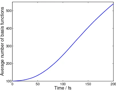
increases the number of trains, which are coupled with each other. Figure 2 shows the growth of

the average number of TBFs in the AIMC simulations. Each of the initial TBFs gives rise to an

average of 4 further TBFs through the cloning process. In the AIMS calculations, each initial

condition spawns an average of 4.1 new TBFs, giving a similar basis set growth rate compared to

AIMC.

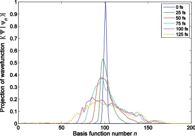
An example of wavefunction spreading over a train basis set with Ntrain=200 for ethylene

is shown in Figure 3. The initial population is localized on the middle “car” of the set of TBFs in

a “train” corresponding to the same initial condition. As time progresses, the window of TBFs

along the trajectory that are being included in the calculation also shifts forward. Thus, the

corresponding population of the “cars” stays localized in the middle TBF, but spreads over the

cars in the train. As Figure 3 shows, for this case, the wavefunction remains largely localized on

the 100 TBFs in the middle of the train. On the basis of this and similar preliminary studies, we

concluded that Ntrain=100 would be sufficient for the MCE and AIMC calculations in this case.

Figure 4 compares the average ground-state population as a function of time given by

MCE and AIMC calculations, with and without basis set expansion using trains. The population

was averaged over 200 non-interacting trajectories with initial conditions randomly generated

from the ground-state vibrational Wigner distribution. The ground-state population evolution

predicted by calculations , with and without train basis functions, is very similar. The results are

somewhat smoother when the train basis set is used, but the difference is within the error bars.

One can conclude that, at least for this problem where the conical intersection is highly peaked

basis set expansion are not pronounced. Of course, one should also recall that this basis set

expansion carries no cost (in the context of ab initio molecular dynamics). Future work will

investigate the degree to which the representation of the nuclear wavefunction is improved by the

use of time-displaced basis set expansion.

The initial population dynamics predicted by MCE and AIMC are similar. However, as

the ground state population increases the predictions begin to deviate, and by 100fs they are quite

different. The relaxation rate predicted by AIMC is significantly faster. This behavior is as

expected – as the population on the ground and excited states becomes nearly equal, the

Ehrenfest dynamics of the TBFs will become that of the average of the two electronic states.

This will tend to keep the TBFs in the region near the conical intersection longer and population

transfer in both directions (to the upper state and to the lower state) will be equally probable.

This is a manifestation of the violations of detailed balance which are a well known difficulty in

Ehrenfest dynamics.16-17 The cloning procedure in AIMC solves this problem by allowing the

TBFs to separate and evolve on adiabatic states.

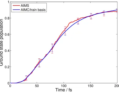
In Figure 5, we compare the results from AIMS and AIMC calculations. The AIMS

results for ethylene have been previously verified by direct comparison to experiment using

CASPT2 for the electronic structure.52Gratifyingly, the AIMC and AIMS methods agree almost

quantitatively on the population dynamics in this case, and are certainly indistinguishable within

the error bars shown.

IV Summary

We propose a new algorithm for quantum molecular dynamics (ab initio Multiple

Cloning or AIMC) which combines the best features of two existing methods: MCE and AIMS.

coherent states in place of the classical equations of motion used in AIMS. Thus, the trajectories

move on an averaged potential energy surface. As is well-known,15 this can lead to problematic

behavior when the electronic states in the average are very different. We alleviate this by

expanding the basis set, similar to spawning, in a procedure we call cloning. As for spawning in

AIMS, cloning does not change the wavefunction – it merely reexpresses it in an expanded

representation. However, itdoeslift the restrictions of the ansatz, i.e. the newly cloned trajectory

basis functions now feel the force appropriate to an adiabatic state and are free to separate.

We have also introduced a new approximation (BAT) for the required matrix elements

that is an alternative to the SPA used in AIMS. The BAT approximation averages truncated

Taylor expansions centered on the two TBFs involved in the matrix element. By comparison, the

SPA evaluates the matrix element by a truncated Taylor series expansion about a single point

intermediate between the position centers of the two trajectory basis functions. The advantage of

the BAT approximation for the matrix element is that it can be computed without any additional

information beyond the energies, gradients, and nonadiabatic couplings at the position centers of

each TBF. There is no need for evaluation of these quantities at intermediate positions. Hence

the number of electronic structure calculations needed scales linearly with the number of TBFs,

as compared to a formally quadratic scaling when the SPA is used.

We have implemented the AIMC algorithm in the AIMS module of the MOLPRO

package and tested it on the benchmark case of photodynamics in ethylene. We showed that the

AIMS and AIMC algorithms give comparable results for the excited state lifetime in this

molecule. In this test case, there does not appear to be any benefit from the use of

advantages to time-displacement in other cases or for more sensitive properties than the

electronic population (e.g. the absorption spectrum60-61or multi-dimensional spectroscopies).

Acknowledgement

This work was supported by EPSRG Grant EP/J001481/1 International Collaboration in

Chemistry: New First Principles Methods for Nonadiabatic Dynamics and NSF CHE-11-24515.

We also gratefully acknowledge Rick Heller who suggested combining features of the AIMS and

Figures

Figure 1. Graphical illustration of the propagation on a small Ehrenfest trajectory guided basis

[image:24.595.86.492.124.443.2]

Figure 2. Growth of the average number of TBFs in an AIMC calculation (with 200 initial

conditions) using trains with Ntrain=100. On average, each TBF produces an additional 4 TBFs

through cloning.

0 50 100 150 200

100 200 300 400 500

Time / fs

A

v

e

ra

g

e

n

u

m

b

e

r

o

f

b

a

s

is

fu

n

c

ti

o

n

[image:25.595.92.490.151.433.2]

Figure 3. Time evolution of ethylene’s wave function in a train basis set. The basis is moving

along a quasi-classical trajectory so that the maximum of amplitude remains in the middle of the

Figure 4. Ground-state population dynamics of ethylene following excitation to the

spectroscopic 1Bu (*) state. . We compare calculations using Ehrenfest dynamics with a

basis of one Gaussian function (MCE), coherent state trains (MCE/train, Ntrain=100), one

Gaussian function with basis function cloning (AIMC), and coherent state trains with basis

function cloning (AIMC/train, Ntrain=100). Results are averaged over 200 initial conditions and

[image:27.595.96.489.124.430.2]

Figure 5. Comparison of time evolution of ground state population after * photoexcitation

from AIMS (red) and AIMC (using trains, Ntrain=100, blue) calculations with

SA-3-CAS(2/2)/6-31G**. Results are averaged over 200 initial conditions and error bars (95% confidence interval)

are shown.

0 50 100 150 200

0 0.2 0.4 0.6 0.8 1

Time / fs

G

ro

u

n

d

s

ta

te

p

o

p

u

la

ti

o

n

AIMS

Appendix 1

The equations for integrals involving complex Gaussian basis functions, which appear in our

formalism, are as follows:

(A1.1)

(A1.2)

(A1.3)

(A1.4)

(A1.5)

(A1.6)

where

D

R

=

R

n

−

R

m,

D

P

=

P

n

−

P

m, Dγ = γ_n−γ_m, R=

R_n+R_m

2 , P=

Pn+Pm

2 .

Appendix 2

Let us consider the ansatz of Eqs. 19-20 for the full wave function

, (A2.1)

where the basis functions are the Ehrenfest configurations composed, as before, of nuclear and

electronic parts:

, (A2.2)

but unlike the standard ansatz in Eq. 2, the electronic part here is “attached” to the center of the

. (A2.3)

Substituting the ansatz (A2.1) into the Schrodinger equation one obtains:

. (A2.4)

The matrix elements are as follows:

, (A2.5)

, (A2.6)

, (A2.7)

where are the kinetic energy matrix elements.

Comparing to Eq. 14, Eq.(A2.6) contains an extra term which includes ;

likewise, comparing to Eq. 16, Eq.(A2.7) does not have the term containing

ϕ

_N

∇

_R

ϕ

_M and

ϕ

_N

∇

_R2

_ϕ

M . The difference is due to the fact that

ϕ

I

=

ϕ

I

(

r

;

R

)

is a function of R and,

therefore, is acted upon by the nuclear kinetic energy operator. On the other hand, the function

depends on the time dependent Rn and therefore is subject to time

differentiation.

Approximations must again be introduced in order to evaluate the matrix elements. As in

function depends weakly on Rk, the position of the nuclei. Then for pairs of basis functions with

sufficient nuclear overlap we can write:

, (A2.8)

, (A2.9)

i.e. the nonadiabatic coupling matrix element between two wave functions localized at points

m

R and Rn is an average between the two “local” nonadiabatic couplings. For m=nit is not an

approximation.

We assume the following approximation for the Born-Oppenheimer potential energy

matrix elements:

(A2.10)

The last two terms can be disregarded because far from intersection the nonadiabatic coupling

terms are small and near the intersection where VI VJ the two terms cancel out. Then using the













                       2 ) ( ) ( 2 ) ( ) ( ~ , ˆ ~( ) ( ) n I n n m m I n m m IJ n I m I n m IJ n n J r el m I m V V V V H R R R R R R R R R r, R

R  

          . (A2.11) As before

χ_m ∂

∂t χn = R

•

n χ_m ∂ ∂Rn

χ_n +P

•

n χ_m ∂ ∂Pn

χ_n 



 



_{. (A2.12)}

Altogether, under the same assumption of smoothness of the electronic wave function and its

weak dependence on the nuclear coordinates, the equations for the amplitudes cnbecome the

same as for those in the ansatz of Eqs. 2-3. The only difference is that the nonadiabatic coupling

term a_Imχ_m a_Jnχ_m R

•

md_IJ

( )

Rm +R

•

nd_IJ

( )

Rn

2

IJ

∑

originates now from the time dependence of the

electronic basis functions but not the kinetic energy operator. Although currently both forms of

the total wave function given by Eqs. 2-3 or Eqs. 19-20 obey the same equation, it is not clear

which of the two approaches will be more convenient for generalization in future, and for the

References

1. Cheng, Y.-C.; Fleming, G. R. Dynamics of Light Harvesting in Photosynthesis. Ann. Rev.

Phys. Chem.2009,60, 241.

2. Blanchet, V.; Zgierski, M. Z.; Seideman, T.; Stolow, A. Discerning vibronic molecular

dynamics using time-resolved photoelectron spectroscopy.Nature1999,401, 52.

3. Collini, E.; Wong, C. Y.; Wilk, K. E.; Curmi, P. M. G.; Brumer, P.; Scholes, G. D. Coherently

wired light-harvesting in photosynthetic marine algae at ambient temperature. Nature2010, 463,

644.

4. Herek, J. L.; Wohlleben, W.; Cogdell, R. J.; Zeidler, D.; Motzkus, M. Quantum control of

energy flow in light harvesting.Nature2002,417, 533.

5. Kuroda, D. G.; Singh, C. P.; Peng, Z.; Kleiman, V. D. Mapping Excited-State Dynamics by

Coherent Control of a Dendrimers Photoemission Efficiency.Science2009,326, 263.

6. Yarkony, D. R. Diabolical conical intersections.Rev. Mod. Phys.1996,68, 985.

7. Lasorne, B.; Worth, G. A.; Robb, M. A. Excited-state dynamics. Wiley Interdiscip.

Rev.-Comput. Mol. Sci.2011,1, 460.

8. Car, R.; Parrinello, M. Unified Approach for Molecular Dynamics and Density-Functional

Theory.Phys. Rev. Lett.1985,55, 2471.

9. Tuckerman, M. E.; Ungar, P. J.; von Rosenvinge, T.; Klein, M. L. Ab initio molecular

dynamics simulations.J. Phys. Chem.1996,100, 12878.

10. Ben-Nun, M.; Martínez, T. J. Ab Initio Quantum Molecular Dynamics. Adv. Chem. Phys.

2002,121, 439.

11. Meyer, H.-D.; Miller, W. H. A classical analog for electronic degrees of freedom in

nonadiabatic collision processes.J. Chem. Phys.1979,70, 3214.

12. Billing, G. D. On the use of Ehrenfest's theorem in molecular scattering. Chem. Phys. Lett.

1983,100, 535.

13. Negele, J. W. The mean-field theory of nuclear structure and dynamics. Rev. Mod. Phys.

14. Tully, J. C.; Preston, R. K. Trajectory surface hopping approach to nonadiabatic molecular

collisions: The reaction of H+ with D2.J. Chem. Phys.1971,55, 562.

15. Tully, J. C. Molecular dynamics with electronic transitions.J. Chem. Phys.1990,93, 1061.

16. Parandekar, P. V.; Tully, J. C. Mixed quantum-classical equilibrium. J. Chem. Phys. 2005,

122, 094102.

17. Parandekar, P. V.; Tully, J. C. Detailed Balance in Ehrenfest Mixed Quantum-Classical

Dynamics.J. Chem. Theo. Comp.2006,2, 229.

18. Schmidt, J. R.; Parandekar, P. V.; Tully, J. C. Mixed quantum-classical equilibrium:

Surface-hopping.J. Chem. Phys.2008,129, 044104.

19. Martinez, T. J.; Levine, R. D. First-principles molecular dynamics on multiple electronic

states: A case study of NaI.J. Chem. Phys.1996,105, 6334.

20. Martinez, T. J.; Levine, R. D. Dynamics of the collisional electron transfer and femtosecond

photodissociation of NaI on ab initio electronic energy curves.Chem. Phys. Lett.1996,259, 252.

21. Martinez, T. J. Ab initio molecular dynamics around a conical intersection: Li(2p)+H2.

Chem. Phys. Lett.1997,272, 139.

22. Ben-Nun, M.; Martinez, T. J. Ab Initio Molecular Dynamics Study of cis-trans

Photisomerization in Ethylene.Chem. Phys. Lett.1998,298, 57.

23. Martinez, T. J.; Ben-Nun, M.; Ashkenazi, G. Classical/quantal method for multistate

dynamics: A computational study.J. Chem. Phys.1996,104, 2847.

24. Martinez, T. J.; Ben-Nun, M.; Levine, R. D. Multi-Electronic-State Molecular Dynamics: A

Wave Function Approach with Applications.J. Phys. Chem.1996,100, 7884.

25. Heller, E. J. Time-dependent approach to semiclassical dynamics.J. Chem. Phys. 1975, 62,

1544.

26. Heller, E. J. Frozen Gaussians: A very simple semiclassical approximation. J. Chem. Phys.

1981,75, 2923.

27. Ben-Nun, M.; Martinez, T. J. Nonadiabatic Molecular Dynamics: Validation of the multiple

spawning method for a multidimensional problem.J. Chem. Phys.1998,108, 7244.

28. Ben-Nun, M.; Martinez, T. J. A Continuous Spawning Method for Nonadiabatic Dynamics

and Validation for the Zero-Temperature Spin-Boson Problem.Isr. J. Chem.2007,47, 75.

29. Shalashilin, D. V.; Child, M. S. Time dependent propagation in phase space. J. Chem. Phys.

30. Shalashilin, D. V.; Child, M. S. The phase space CCS approach to quantum and semiclassical

molecular dynamics for high-dimensional systems.Chem. Phys.2004,304, 103.

31. Burghardt, I.; Meyer, H. D.; Cederbaum, L. S. Approaches to the approximate treatment of

complex molecular systems by the multiconfiguration time-dependent Hartree method. J. Chem.

Phys.1999,111, 2927.

32. Worth, G. A.; Burghardt, I. Full quantum mechanical molecular dynamics using Gaussian

wavepackets.Chem. Phys. Lett.2003,368, 502.

33. Worth, G. A.; Robb, M. A.; Lasorne, B. Solving the time-dependent Schrodinger equation

for nuclear motion in one step: direct dynamics of non-adiabatic systems. Mol. Phys.2008, 106,

2077.

34. Ben-Nun, M.; Martinez, T. J. Photodynamics of ethylene: ab initio studies of conical

intersections.Chem. Phys.2000,259, 237.

35. Yang, S.; Coe, J. D.; Kaduk, B.; Martinez, T. J. An ``optimal'' spawning algorithm for

adaptive basis set expansion in nonadiabatic dynamics.J. Chem. Phys.2009,130, 134113.

36. Levine, B. G.; Coe, J. D.; Virshup, A. M.; Martiinez, T. J. Implementation of ab initio

multiple spawning in the Molpro quantum chemistry package.Chem. Phys.2008,347, 3.

37. Saita, K.; Shalashilin, D. V. On-the-fly ab initio molecular dynamics with

multiconfigurational Ehrenfest method.J. Chem. Phys.2012,137, 8.

38. Shalashilin, D. V. Multiconfigurational Ehrenfest approach to quantum coherent dynamics in

large molecular systems.Faraday Disc.2011,153, 105.

39. Shalashilin, D. V. Nonadiabatic dynamics with the help of multiconfigurational Ehrenfest

method: Improved theory and fully quantum 24D simulation of pyrazine. J. Chem. Phys. 2010,

132.

40. Shalashilin, D. V. Quantum mechanics with the basis set guided by Ehrenfest trajectories:

Theory and application to spin-boson model.J. Chem. Phys.2009,130.

41. Bittner, E. R.; Rossky, P. J. Quantum decoherence in mixed quantum-classical systems:

Nonadiabatic processes.J. Chem. Phys.1995,103, 8130.

42. Prezhdo, O. V.; Rossky, P. J. Mean-field molecular dynamics with surface hopping.J. Chem.

Phys.1997,107, 825.

43. Ben-Nun, M.; Martinez, T. J. Exploiting temporal nonlocality to remove scaling bottlenecks

44. Shalashilin, D. V.; Child, M. S. Basis set sampling in the method of coupled coherent states:

Coherent state swarms, trains and pancakes.J. Chem. Phys.2008,128, 054102.

45. Ronto, M.; Shalashilin, D. V. Numerical Implementation and Test of the Modified

Variational Multiconfigurational Gaussian Method for High-Dimensional Quantum Dynamics.J.

Phys. Chem. A.

46. Doltsinis, N. L.; Marx, D. First Principles Molecular Dynamics Involving Excited States and

Nonadiabatic Transitions.J. Theo. Comp. Chem.2002,01, 319.

47. Roos, B. O. The Complete Active Space Self-Consistent Field Method and Its Applications

in Electronic Structure Calculations.Adv. Chem. Phys.1987,69, 399.

48. Lengsfield, B. H., III; Yarkony, D. R. Nonadiabatic interactions between potential energy

surfaces: Theory and applications.Adv. Chem. Phys.1992,82, 1.

49. Roos, B. O. Theoretical Studies of Electronically Excited States Using Multiconfigurational

Perturbation Theory.Acc. Chem. Res.1999,32, 137.

50. Mori, T.; Glover, W. J.; Schuurman, M. S.; Martinez, T. J. Role of Rydberg States in the

Photochemical Dynamics of Ethylene.J. Phys. Chem. A2012,116, 2808.

51. Tao, H.; Levine, B. G.; Martinez, T. J. Ab initio multiple spawning dynamics using

multi-state second-order perturbation theory.J. Phys. Chem. A2009,113, 13656.

52. Tao, H.; Allison, T. K.; Wright, T. W.; Stooke, A. M.; Khurmi, C.; van Tilborg, J.; Liu, Y.;

Falcone, R. W.; Belkacem, A.; Martinez, T. J. Ultrafast internal conversion in ethylene. I. The

excited state lifetime.J. Chem. Phys.2011,134, 244306.

53. Sension, R. J.; Hudson, B. S. Vacuum ultraviolet resonance Raman studies of the excited

electronic states of ethylene.J. Chem. Phys.1989,90, 1377.

54. Cromwell, E. F.; Stolow, A.; Vrakking, M. J. J.; Lee, Y. T. Dynamics of ethylene

photodissociation from rovibrational and translational energy distributions of H2 products. J.

Chem. Phys.1992,97, 4029.

55. Stert, V.; Lippert, H.; Ritze, H. H.; Radloff, W. Femtosecond time-resolved dynamics of the

electronically excited ethylene molecule.Chem. Phys. Lett.2004,388, 144.

56. Viel, A.; Krawczyk, R. P.; Manthe, U.; Domcke, W. Photinduced dynamics of ethene in the

N, V, and Z valence states: A six-dimensional nonadiabatic quantum dynamics investigation. J.

57. Viel, A.; Krawczyk, R. P.; Manthe, U.; Domcke, W. The sudden-polarization effect and its

role in the ultrafast photochemistry of ethene.Ang. Chem. Int. Ed.2003,42, 3434.

58. Kosma, K.; Trushin, S. A.; Fuss, W.; Schmid, W. E. Ultrafast dynamics and coherent

oscillations in ethylene and ethylene-d(4) excited at 162nm.J. Phys. Chem. A2008,112, 7514.

59. Thompson, A. L.; Punwong, C.; Martinez, T. J. Optimization of width parameters for

quantum dynamics with frozen Gaussian basis sets.Chem. Phys.2010,370, 70.

60. Ben-Nun, M.; Martinez, T. J. Electronic absorption and resonance Raman spectroscopy from

Ab Initio Quantum Molecular Dynamics.J. Phys. Chem. A1999,103, 10517.

61. Sulc, M.; Hernandez, H.; Martinez, T. J.; Vanicek, J. Relation of exact Gaussian basis

methods to the dephasing representation: Theory and application to time-resolved electronic