Joint contour nets

This is a repository copy of

Joint contour nets

_.

White Rose Research Online URL for this paper:

http://eprints.whiterose.ac.uk/79282/

Version: Accepted Version

Article:

Duke, DJ and Carr, H (2013) Joint contour nets. IEEE Transactions on Visualization and

Computer Graphics. ISSN 1077-2626

https://doi.org/10.1109/TVCG.2013.269

[email protected] https://eprints.whiterose.ac.uk/

Reuse

Unless indicated otherwise, fulltext items are protected by copyright with all rights reserved. The copyright exception in section 29 of the Copyright, Designs and Patents Act 1988 allows the making of a single copy solely for the purpose of non-commercial research or private study within the limits of fair dealing. The publisher or other rights-holder may allow further reproduction and re-use of this version - refer to the White Rose Research Online record for this item. Where records identify the publisher as the copyright holder, users can verify any specific terms of use on the publisher’s website.

Takedown

If you consider content in White Rose Research Online to be in breach of UK law, please notify us by

Joint Contour Nets

Hamish Carr,

Member, IEEE,

and David Duke,

Member, IEEE,

Abstract—Contour Trees and Reeb Graphs are firmly embedded in scientific visualization for analysing univariate (scalar) fields. We

generalize this analysis to multivariate fields with a data structure called theJoint Contour Netthat quantizes the variation of multiple

variables simultaneously. We report the first algorithm for constructing the Joint Contour Net, and demonstrate some of the properties that make it practically useful for visualisation, including accelerating computation by exploiting a relationship with rasterisation in the range of the function.

Index Terms—Computational Topology, Contour analysis, Contour Tree, Reeb graph, Reeb space, Joint Contour Net, Multivariate.

✦

1

I

NTRODUCTION

S

Imulations of physical phenomena have three major

types of data: scalar, vector and multi-variate (multi-field). For scalar and vector data, many visualization techniques exist, from colour maps and glyphs to feature recognition and display. In recent years, these tools have included topological analysis to support visualization both analytically and algorithmically.

Research has only just begun to analyse the topological relationships of two or more properties. We report on the Joint Contour Net, an extension of the Reeb graph, that expresses the relationship between subsets of the domain with common properties. Developing this representation depends on early notions of the contour tree as the rela-tionship between explicit contours or regions, however, rather than working directly from Morse Theory.

2

S

CALAR

F

IELD

T

OPOLOGY

For a scalar function f on a continuous d-manifold M, a level set for isovalueh∈IR is the inverse image ofh:

f−1_{(h) ={x∈M :f(x) =h} (1)}

In 2D, level sets are referred to asisolines, and in 3D, as isosurfaces. Since a level set may not be fully connected, we call a single connected component a contour. For a Morse functionf, contours have one dimension less than the original manifold: e.g. contour lines on a topographic map have one dimension where the surface has two.

In practice, continuous Morse functions with infinite differentiability are intractable, and computational topol-ogy uses piecewise-continuous functions which may or may not be differentiable. These are usually defined on a mesh composed of polygonal, polyhedral or polytopal cells, where the value of f is only known at the vertices of the mesh. Morse behaviour is assured by simulation of simplicity [21], simulation of differentiability [20],

• H. Carr and D. Duke are with the School of Computing, University of Leeds, Leeds, UK.

E-mail:{h.carr,D.J.Duke}@leeds.ac.uk

and/or Discrete Morse Theory [22], which provides a combinatorial equivalent of Morse functions, recon-structing a smooth function for the purposes of analysis. An alternate approach to constructing a smooth func-tion is to work with a quantized representafunc-tion (i.e. discretized in the range of the function). Weber et al. [45] relaxed the constraint of unique values, collecting iso-valued regions and using them for topological analysis, an approach later extended to arbitrary dimension by Allili et al. [1]. More recently, Duffy et al. [14] have recognized that quantization of values in the range must also be taken into account: we will defer this to Section 5. One form of analysis is the Reeb graph [34], which contracts contours to points, giving a graph description of connectivity. For simple domains, this is the contour tree [3]. Both structures are important in graphics and visualization because they capture the relationships of all contours of a function. Moreover, their combinatorial structure, based on equivalence classes between con-tours, subdivides the domain into regions of common behaviour, an important property for analysing data. They have been used for acceleration of isosurface algo-rithms [9], volume rendering [44], comparison of surface shapes [27] and of protein molecules [46], topological simplification of data sets [9], and reduction of high-dimensional data to landscape representations [43], [23]. Van Kreveld et al. [41] computed the contour tree for a mesh of N simplices in O(NlogN) time in two dimensions, O(N2

For the Reeb graph, Pascucci et al. [33] gave a fast streaming algorithm editing the Reeb graph locally as simplices are added to a 2-manifold. While worst case runtime is at leastO(N2

), this is rare, and the algorithm is fast in practice. More recently, Tierney et al. [40] computed the Reeb graph in O(N2

) by cutting a vol-umetric mesh along contours, applying the contour tree algorithm of Carr et al. [8], then repairing the cuts to con-struct the Reeb graph. Doraiswamy and Natarajan [12] have since extended this to arbitrary dimensions and reduced the memory overhead to O(N), thus making the algorithm more efficient in practice. Most recently,

O(NlogN)time algorithms have also been described for both contour trees and Reeb graphs[24], [31], although earlier algorithms may still outperform them in practice.

3

M

ULTI

-V

ARIATE

T

OPOLOGICAL

A

NALYSIS Although multi-variate computational topology is in its infancy, but four approaches can be identified: Jacobi sets, Reeb graph comparison, Reeb spaces, and range tessellation. For clarity, we will use multi-field to refer to functions of the form IRd→IRr, and multivariate data to refer to computational discretizations of multi-fields, although this distinction is not common in the literature. Jacobi sets were described by Edelsbrunner and Harer [17] as the systematic variation of critical points in multi-fields. These are extracted by taking a contour with respect to one variable, restricting another variable to that contour, and finding the critical points of the restricted function. As the first variable varies, the critical points sweep out paths in the domain. Moreover, Jacobi Sets can also be defined for time-varying data sets, and constructed in polynomial time [18]. Jacobi Sets can be simplified with rules similar to the contour tree [30].

A second approach uses the Reeb graph and contour tree to compare scalar fields. Hilaga et al. [27] used graph matching on Reeb graphs of different 2-manifolds to recognize shape similarities. Zhang et al. [46] extended this to3-manifold functions, computing the contour tree with quantized data, then graph matching to recognize similar molecular shapes as expressed in the electrostatic potential field. Schneider et al. [37] took contour trees for two properties in a simulation, simplified the contour trees, then compared the overlap of features defined in the contour tree. While these papers have shown that the Reeb graph / contour tree can be used for comparison, they merely identify similarities between individual fields rather than giving overall structure.

A third approach starts by extending the Reeb graph to multivariate functions. Edelsbrunner et al. [19] did so, calling the result the Reeb space. We will illustrate an example of a Reeb space in Section 4, but observe that this is tightly linked with the mathematical analysis of singular fibers [35]. This analysis has been completed for functions of the form IR3→IR2 and IR4→IR3, but has not been accompanied by an algorithm for computation. Edelsbrunner et al. [19] reported a complex and math-ematically formalised algorithm for the Reeb space,

lacking implementation details and asymptotic analysis. Moreover, the algorithm reported only works for 4 or fewer variables. In contrast, our approach works on principle for an arbitrary number of variables. More recently, Carlsson et al. [5] generalised a related notion, persistence, to higher dimensions. Their algorithm, how-ever, isO(m2

n4

)wherenis the number of properties and

mis the number of cells in the input complex.

A fourth approach observed that statistics of isosur-faces were closely related to histograms [6]. Further developed by inverse gradient weighting [36], the latest work has shown that the relationship is defined by formal models of integration over interval volumes [14], typically defined by unit intervals in the range. This approach was used to improve scatterplot visualisations of continuous phenomena by using graphics hardware to project tetrahedra into the range of a function [2]. The relevance of this line of work is that it projects the graph of the function from an m+n-dimensional embedding space. As we will see later, this provides a method for accelerating computation of the Joint Contour Net.

In short, while some work has been done on multi-variate topological analysis, what is lacking is a simple, efficient algorithm that computes usable structures. We report such an algorithm for the Joint Contour Net or JCN, which computes an approximate representation of multi-variate topology. Where m > n, the JCN is an approximation of the Reeb space. For m =n, the Reeb space is identical to the manifold of the function, but for

m < n, the Reeb space is undefined. This is of particular concern when analysing scientific data, as it is common to compute many properties on a grid, so thatm << n. In contrast to the Reeb space, since the JCN is based on explicit subdivision of geometry, it can be computed even whenm≤n. For such cases, however, the JCN does not compute either the Reeb space or an approximation to it. Instead, it computes a graph representation of a remeshed version of the input data. We will, however, defer discussion of the details of this until Section 7, and start by generalising the notion of contour contraction.

4

G

ENERALIZED

C

ONTOUR

C

ONTRACTION

It is straightforward to extend level sets to multi-variate functions. Instead of a scalar functionf :IRm→IR, we shall consider scalar functions of the formf :IRm→IRn, and define a level set for an isovalueh∈IRn to be:

f−1_{(h) ={x∈M ⊆IR}m_{:f(x) =h} (2)}

As before, a contour is a connected component of a level set: one method of constructing the level set for a multi-variate isovalue h= (h1, . . . , hn)is to decompose

f into scalar functions f1, . . . , fn, and take the level set

f−1

1 (h1) of the first component h1 of the isovalue. As

an example, we will define a bivariate function f :A⊂

IR3 → IR2 where A = [−1,1]×[−1,1]×[0,1], and f = (f1, f2), wheref1(x, y, z) =

p

x2_+y2_+z2 _{is a spherical}

0.25 0.50 0.75 1.00 1.25 1.50 1.75 2.00

arbitrary

1 2 3 4 5 6

0.25

0.50

0.75

1.00

f1 h1

1 −

( )

f1 h1 f2 h2

1 1 − −

∩

( ) ( )

IR

3

Contour lines of f1 restricted to f2 1_{( )h}

(

)

Contour trees of f1 restricted to f2 1_{( )h}

(

)

Contour lines of

f₂ restricted to f₁1_{( )h}

(

)

Contour trees of

f₂ restricted to f₁1_{( )h}

(

)

Joint Contours can be found by intersecting contours of the individual functions: here, a single hemispherical contour of f1 (distance) is shown with

a joint contour found by intersection with a planar contour of f2 (z-height) f1 (distance)

[image:4.612.53.566.59.493.2]

f2 (z-height)

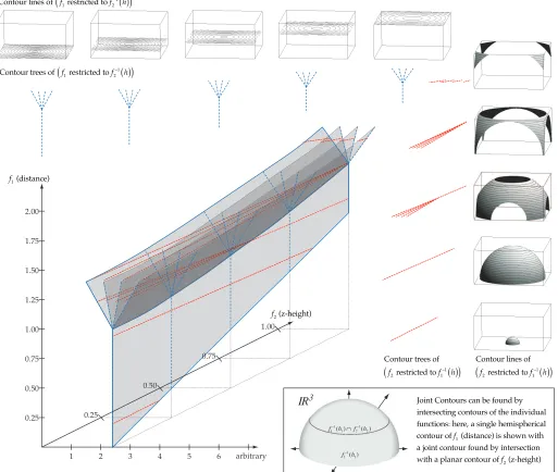
Fig. 1: The variation in level sets of a bivariate function can be expressed as a2-manifold. Here, the functionf1 is

a distance field, and the functionf2 is a height field. If we take an isosurface off1then compute the Reeb graph of

f2 restricted to that surface, we get the sequence shown on the right. If we take an isosurface off2 then compute

the Reeb graph of f1 restricted to that surface, we get the sequence displayed along the top. Note that the Jacobi

Set in this example is a subset of the edges of the Reeb Space projected back into the domain of f.

linear inz. As shown in Figure 1, the level sets off1 are

hemispheres. We take as a second function f2(x, y, z) =

z, whose level sets are planes parallel to z = 0. Then, where the domain of the function is a 3-manifold, the level sets of f1 and f2 are 2-manifolds, possibly with

boundary, and the level sets of f are 1-manifolds.

Figure 1 shows a small example of a bivariate function combining a distance function as f1 and a height

func-tion as f2. Isosurfaces of f1 are hemispheres truncated

to the domain A, (right). We show contours of f2 on

these isosurfaces, and their contour trees. As h1 varies,

the Reeb graph sweeps out the Reeb space, as shown. Equally, we can fix h2 to get isosurfaces of f2, in this

case flat sheets. Plotting the contours of f1 on these

sheets, we get the sequence along the top. Here, the Reeb graph remains combinatorially consistent across all isovalues, but the values of the critical points change, and unsurprisingly, the Reeb space is again swept out.

As with the Reeb graph, any contour of f contracts to a point on the Reeb Space. And, since Jacobi Sets track the evolution of critical points of one property with respect to level sets of another, it then follows that the Jacobi Sets in this representation are a subset of the edges of the Reeb Space. To be precise, the critical points of f1 or f2 trace out the internal edges of the

8 4 3 7 5 6 1 2 9 8 5 6 7 4 3 4 6 7 8 9 3 2 1

7 8 9

4 1 5 2 6 3 3 9 5 1 2 4 6 7 8 9 1 5 9 1 8 3 (3,1) (4,1) (3,2) (4,2) (4,3)

[image:5.612.52.299.49.313.2]

(5,2)(6,2) (7,2) (4,4) (5,4) (6,5) (7,6) (8,7) (7,7) (6,6) (5,5) (6,7) (5,4) (6,4) (6,3) (7,4) (8,3) (9,3) (3,5) (1,8) (1,9) (4,9) (3,9) (2,9) (6,8) (3,6) 8/7 4/4 3/1 1/9 2/6 9/3 6/2 7/8 (1,9) (2,9) (8,7) (3,1) (9,3)

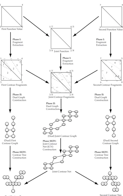
Fig. 2: Contour trees & JCN where f : IR2 → IR2. Note how the JCN retessellates the manifold based on properties of the range rather than of the domain.

extreme values of the domain. In Figure 3, for example, computing the Jacobi set by analysing critical points of

f2on isosurfaces off1extracts all non-manifold edges of

the Reeb space, but doing so by analysing critical points of f1 on isosurfaces of f2 does not extract the edges

at minimum and maximum values of f2. This occurs

because the formal definition of Reeb space assumes a manifold without boundary, where our example has boundaries. Moreover, the Jacobi Set is usually shown in the domain off, rather than in the Reeb Space.

This process of contracting contours to points has a drawback. Each time we fix an isovalue, we reduce the dimensionality of the graph of the function M by one. Thus, for m ≤ n, our level sets will in general have dimension zero (points) or be empty, and the Reeb space will be the original manifold M.

5

F

RAGMENTS AND

S

LABS

Following Hilaga et al. [27], we use connected compo-nents of interval regions instead of contours. As ob-served by Duffy et al. [14], these are of full dimension, allowing intersection without dimension loss.

In Figure 2, we show a simple two-dimensional exam-ple. Here, instead of contour lines, we consider quantised contours: note how the dashed lines divide the mesh into regions of uniform connectivity. For clarity, we will use fragmentto refer to such a region in a single cell, butslab to refer to such a region with respect to the entire mesh. Since fragments are adjacent across cell boundaries, we collect them across cells to compute the contour tree,

as shown on the sides of Figure 3. For quantized data on a simplicial mesh, the resulting tree is identical to the contour tree for a suitable choice of quantization.

For multi-variate data, we intersect slabs, as in Fig-ure 3. We define a Joint Level Setat isovalueh∈ZZn as:

f−1_{(h) ={x∈M :round(f(x)) =h} (3)}

For simplicial meshes, Joint Level Sets are not always connected, so we define a slab to be a single connected component of a Joint Level Set, in the same way that a contour is a single connected component of a level set.

In practice, we assume f is piecewise linear over a simplicial mesh. The slabs in each simplex are convex polytopes of full dimension - polygons in 2D, polyhedra in 3D. Combining the Joint Slabs of all simplices gives a slab decomposition of the entire domain, where adjacent slabs may or may not share the same discrete isovalue(s).

6

J

OINT

C

ONTOUR

N

ETS

After extracting fragments for each simplex, each slab in the entire mesh is a union of connected fragments in different simplices. By computing fragment connectivity, we can therefore identify the slabs.

Since fragments are adjacent between cells, the Joint Contour GraphGis their dual graph. Here, nodes repre-sent fragments and edges reprerepre-sent adjacencies. We then see that slabs are equivalent to connected components of isovalued nodes in the Joint Contour Graph.

We now perform a final reduction to find the con-nected components of each Joint Level Set, applying Tar-jan’s union-find [39] to edges of the Joint Contour Graph between isovalued nodes. This contracts components as identified by Reeb [34], and results in the Joint Contour NetorJCN, an abstraction which captures the systematic variation of all propertiessimultaneously.

Expressed in pseudo-code, the JCN algorithm consists of four phases: division of the domain into fragments, construction of the Joint Contour Graph G, union-find to find slabs (i.e. nodes in the JCNJ), and a final phase to identify the edges of J. In practice, Phases I and II can be combined, as can Phases III and IV.

In Phase I, we start off with the meshM0=M. At each

iteration of Steps 4-8, mesh Mi₋1 has each cell divided

with respect to propertyfi, generating a new subdivided

mesh Mi at each stage. When complete,Mn then holds

the Joint Contour Slabs as defined above.

Phase II then constructsGfrom the fragment adjacen-cies. In practice, this will actually be computed during Phase I as part of the mesh data structure.

Phase III then applies Union-Find to identify the nodes of J. Initially, each representative in the Union-Find corresponds to a fragment - i.e. a node of G. As each fragment Ka is processed, each neighbour Kb is

examined. Iffi(Ka) =fi(Kb)for alli, then the fragments

1/7 3/6 2/8 4/5 1 3 2 4

First Function Value

7

6 8

5

Second Function Value

Joint Function 1 3 2 4 1.5 1.5 1.5 2.5 3.5 2.5 3.5 2.5 2.5 2 3 4 3 2 1 1 7 5 8 6 6.5 6.5 6.5 6.5 7.5 7.5 7.5 5.5 5.5 6 7 8 8 7 6 5

First Contour Fragments Second Contour Fragments

1/7 3/6 2/8 4/5 2/7 3/7 2/6 3/6 2/8 1/7 1/7 2/7 2/8 2/6 3/6 3/7 4/5 4/6 3/5

Joint Contour Fragments

4/5 3/5 4/6 3/6 2/6 3/7 2/7 1/7 2/8 2/7 1/7 2/8 2/6 3/7 3/6

(Dual) Joint Contour Graph

4/5 3/5 4/6 3/6 2/6 3/7 2/7 2/7 1/7 2/8 2/6 3/7 3/6

Joint Contour Net

4 3 3 2 1 2 1 8 8 7 7 6 6 5 (Dual) First Contour Graph (Dual) Second Contour Graph 4/5 3/5 4/6 3/6 2/6 3/7 2/7 1/7 2/8 2/7 2/6 3/7 3/6 4/5 3/5 4/6 3/6 2/6 3/7 1/7 2/7

2/8 2/7

2/6 3/7

3/6

First Contour Tree Second Contour Tree

[image:6.612.102.511.42.691.2]

Phase I: Fragment Extraction Phase I: Fragment Extraction Phase I: Fragment Extraction Phase II: Dual Graph Construction Phase II: Dual Graph Construction Phase II: Dual Graph Construction Phase III/IV: Contour Tree Construction Phase III/IV: Contour Tree Construction Phase III/IV: Joint Contour Net (JCN) Construction

Algorithm 1Algorithm for Computing JCN

Require: For simplicial mesh M with functions

f1, . . . , fn sampled to integer values at vertices of

M, compute Joint Contour NetJ

1: PHASE I: CREATE FRAGMENTS

2: SetM0=M 3: fori= 1 tondo

4: for allCellsK∈Mi−1 do

5: Initialize subdivided meshMi← ∅ 6: forj=min(fi|K)tomax(fi|K) do

7: Add fragmentKT

f−1([j−0.5, j+ 0.5])toM_i

8: end for

9: end for

10: end for

Ensure: Mn holds the fragmentsFi off

11:

12: PHASE II: COMPUTE JOINT GRAPHG

13: forevery fragmentFi inMn do

14: forevery fragmentFj adjacent toFi do 15: ConnectF1, F2 in G

16: end for

17: end for

Ensure: Gis the dual graph of the fragments

18:

19: PHASE III: COMPUTE NODES OF JCNJ

20: Let Nf =Size(Mn)be the number of fragments in

Mn

21: fora= 1 toNf do

22: Initialize Union-Find:U(a) =a

23: end for

24: fora= 1 toNf do

25: for allcellsKb∈Mn adjacent toKa do

26: iffi(Ka) =fi(Kb)∀1≤i≤nthen 27: Union(U, a, b): Adde= (a, b)toU

28: end if

29: end for

30: end for

Ensure: The representatives ofU are the slabs

31:

32: PHASE IV: COMPUTE EDGES OF JCNJ

33: fora= 1 toNf do

34: IfU(a) =a, addaas node to J

35: end for

36: for alledges(Kb, Ka)∈Gdo

37: iffi(Ka)6=fi(Kb)for any1≤i≤nthen 38: Add edge(U(a), U(b))to J

39: end if

40: end for

Ensure: J now holds the Joint Contour Net

Finally, Phase IV strips out connected components of

U to be used as nodes inJ, then iterates through all cells

Ka, Kb. For each pair of cellsKa, Kbthat are which share

a common m−1 dimensional face but do not share all isovalues, Ka cannot be in the same component ofU as

Kb, so an edge is added between their representatives

in J (if already present, this operation has null effect). When complete, the JCNJ has been constructed.

6.1 Algorithmic Analysis

To analyse this algorithm, we observe that it is depen-dent on the number N of simplices in the input mesh, the numberQiof levels of quantization for each function

fi, the number r of functions defined, and the number

dof input dimensions.

In Phase I, the loops over d and over the cells are functionally independent, so we assume each cellK∈M

is subdivided d times. The analysis then depends on the number of cells produced by intersectingQ1, . . . , Qd

fragments. Barycentric interpolation of f on the simpli-cial mesh means that each set of fragments has parallel cuts: an easy upper bound on the number of fragments isk =Qd

i=1Qi, although finer analysis might be found

in the extensive literature on ham-sandwich cuts [16]. Accordingly, an upper bound on the computation time for Phase I is O(rNf) time where Nf = O(kN). Here,

the factor of r is because each cell isr-dimensional, so insertion of new cells is assumed to takeO(r) time.

Phase II iterates over every fragment in the mesh, then over every adjacent fragment. Assuming that retrieving each pair of adjacent fragments takesO(1)time, as does storing them in the graph G, then this phase takes

O(Ne+Nf) time, where Ne is the number of edges in

G, i.e. the number of adjacencies between fragments. While graph connectivity means that Ne may be

O(N2

f), a tighter bound exists. As we will see in Section 7,

each fragment is the projection of a hypercube in the range onto the graph of the function - i.e. a form of rasterisation. Thus, each fragment is a convex distorted hypercube, possibly intersecting faces of the simplex.

Now, a hypercube of dimension r has 2r faces, and each side of the simplex can only add one face by trun-cation. Thus, each fragment can have at most2r+d+ 1

faces, each of which contributes at most one edge to

G. Thus, Ne = O((2r +d)Nf), which is

dimension-dependent but not quadratic in the number of fragments. Phase III performs a Union-Find to identify slabs (nodes in the JCNJ). Here, each adjacency is considered twice, but comparingnfields means that the cost will be

O(r) each time, for an overall cost ofO(rNe). However,

once the comparison is complete, at mostNe edges will

be added to the union-find structure, giving an overall cost for this phase of O(rNe+Neα(Ne)), whereα(x) is

the slow-growing inverse Ackermann function [39]. Phase IV iterates through the Union-Find U in at most Nfα(Nf) time to extract the vertices of J, then

iterates through the adjacencies. Each comparison may take O(r) time, giving at most O(rNe) time. Adding

edges to J however is assumed to take O(1) time, for an additional time of O(Ne), which can be subsumed.

Phase IV therefore takesO(Nfα(Nf)+rNe)time in total.

Adding the costs, we getO(Nf)+O(Ne+Nf)+O(rNe+

Neα(Ne))+O(Nfα(Nf)+rNe). SinceNe=O((2r+d)Nf),

While this is polynomial, the upper bound is very loose: the algorithm is primarily sensitive to k, the product of the number Qi of quantization levels of the

properties. Recent work [13] has shown that up to 95%

of cells have only one quantization level, and most cells only have a few quantization levels. As a result, the worst-case behaviour is likely to occur only in a small number of cells, and can probably be bounded by examining the Jacobian of the function [14].

7

P

ROPERTIES

The JCN has a number of interesting properties that are likely to be useful for multi-variate analysis. Some of these properties are essentially theoretical and or algorithmic, while others are practical and related to known visualization tasks.

7.1 Theoretical Properties

It should be clear from the discussion in previous sec-tions that the JCN and the Reeb Space are effective generalisations of the Reeb Graph and the Contour Tree and closely related to the analysis of singular fibers. Thus, the JCN can be viewed as part of the iterative process by which we explore the relationship between formal analysis, algorithmic development, and practi-cal computations. Since the implications are broad, we list some of the issues we have identified, along with sketches of potential developments.

Reeb Graph / Contour Trees: Good generalisations

can often be reflected back to the original example to develop further insights. Since the JCN generalizes Reeb Graph computations, new algorithms may be expected, although the work of Hilaga et al. [27] can now be recognized as essentially the same computation..

Pascucci showed a sort-based Ω(tlog(t)) bound on contour tree computation [42]. However, quantization in the form of the radix sort escapes the generalO(tlog(t))

bound on sorting. Since the JCN algorithm exploits quantization, so this lower bound does not apply.

A less obvious point is that most existing Contour Tree and Reeb graph algorithms rely on a global sort order of the vertices, and that this global property hampers parallel computation. Our algorithm processes each sim-plex independently in Stage I: as a form of rasterisation, fragment creation can be parallelized. While further work is needed to produce an efficient implementation, the absence of any global ordering means that the new algorithm can be expected to parallelize relatively easily. The mapping from discrete fragments onto JCN nodes should replace the global sorting step of existing algo-rithms with a radix sort, which is easy to parallelize.

Re-meshing:As identified by an anonymous reviewer,

the effect of the fragment and slab computation is to retessellate the function with respect to range properties instead of domain properties. To see this, consider the bottom row of Figure 2, in which the left hand image shows the original mesh with each cell broken up into

fragments, and the middle image shows the slabs. Since these slabs fill the space, they constitute a remeshing of the domain. Moreover, one can project them onto the graph Gr(f) of the function and observe that each slab constitutes an identifiable fragment ofGr(f).

However, since this small example isIR2→IR2,Gr(f)

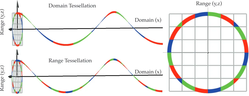
is embedded in IR4, which is difficult to illustrate. We instead show a simplified example in Figure 4 of a function g : IR → IR2: i.e. a space curve in IR3, in this instance a helix, i.e. g(x) = (y =cosx, z =sinx). Since our fragments and slabs are defined by taking intervals in the ranges ofy, z, the effect of this is to retessellate the graph into the coloured segments shown (note that they have no thickness except for the purposes of illustration). Given this retessellation, we can now see that as the number of slabs increases, the tessellation will converge to the original space, with each coloured region in general representing a slab composed of one or more fragments. And, since the JCN is the dual edge graph of these slabs, convergence to the connectivity of the Reeb Space then follows, although true convergence requires handling higher-order faces as well.

Relationship to Reeb Space:In Section 4, we observed

that m > n, m = n and m < n need to be treated separately. Form > n, the Reeb Space, the JCN and the singular fiber analysis are well defined, and the JCN is an approximation of the connectivity of the Reeb space. Form=n, joint contours or fibers (i.e. inverse images of values in the range) will in general be of dimension0

- i.e. finite collections of individual points, and the Reeb space is identical to the graph of the function. For the same reason, singular fiber analysis does not handle this case at present. The JCN, however, can still be computed, as it is explicitly based on geometric subdivision.

Form < n, no Reeb space is defined, but the JCN can still be computed, as shown in Figure 4. Since the JCN remeshesGr(f), and varying mesh representations is of practical value, we expect that geometric [9] information can be captured and analysed this way.

For example, in the JCN, the density (resolution) of the tessellation will be related to the rapidity with which the quantization changes - i.e. to the Jacobian off. We note that high gradients in volumetric data lead to aliasing problems, and observe that, in previous work, aliasing was resolved by exploiting continuity [14]. As a result, we may be able to look at local correlation of variables by examining the density in the domain of the slabs. Second, there may be graph algorithms which use prop-erties of the JCN to identify boundaries that do not map to isovalued boundaries or Joint Contours. And third, the slab density and the related graph representation may still be useful even for cases where m < n, and the Reeb Space is equivalent to the original domain.

7.2 Practical Properties

Rang

e (y

,z)

Domain (x)

Domain (x)

Rang

e (y

,z)

Range (y,z)

Domain Tessellation

[image:9.612.51.555.58.252.2]

Range Tessellation

Fig. 4: A function g :IR→IR2 that defines a helix. At left, Gr(g) is shown as a space curve, once with segments coloured by uniform tessellation of the domain (top), once coloured by uniform tessellation of the range (below). At right,Gr(g)shown by projection into the range: the same coloured segments now become fragments with respect to the range, even though multiple components may project to the same range cell. As a result, computation of the JCN is equivalent to rasterising Gr(g) with respect to pixels in the range (as with Continuous Scatterplots [2]. Note that the segments are of zero thickness, but are exaggerated for the purposes of illustration.

properties of the Reeb Graph / Contour Tree, or to potential visualization tasks:

Representation of Multi-Variate Contours:Each

uni-variate or multi-uni-variate contour corresponds to a con-nected set in the JCN. This follows directly from the characterization of the slabs as equivalence classes of contours used in the proof above.

Extraction of Contours: Either uni-variate or

multi-variate slabs can be extracted using the JCN. Again, from the characterization of the slabs as equivalence classes of contours, this follows provided that we store a single fragment as a representative of each slab (i.e. node in the JCN). Extracting a contour can then be done with depth-first or breadth-first search through the cells of the mesh, following to adjacent fragments. Alternately, since the fragment adjacency is encoded in the Joint Contour Graph, a simple flood-fill can be used to extract all relevant fragments.

Contours and Features: Uni-variate contours cut the

domain into pieces, thus defining features: moreover, the nesting relationship induced by this property is one of the definitions of the Contour Tree [3]. Most multi-variate contours, however, do not cut the domain into pieces. However, and perhaps more interestingly, not all algorithms use contours. Instead, methods such as level sets use alternate formulations to construct boundary surfaces that separate an inside from an outside, or otherwise segment the domain into features.

Given any such boundary that cuts the domain into pieces, let B be the set of slabs through which the boundary passes. SinceB is a superset of the boundary, removing it will also disconnect the domain. Since each

slab corresponds to a JCN node, removing the nodes corresponding to B must also disconnect the JCN.

Inversely, since each node in the JCN represents a slab in space, and the edges of the JCN represent face-adjacencies of the slabs, a connected setN of nodes in the JCN represents a contiguous region of the domain. And, if N is a cut set for the JCN, each cut component will correspond to a disjoint region of the domain - hence, cut sets in the JCN induce cuts in the domain that separate potential features. It then follows that graph properties such as minimal cut sets in the JCN are likely to reveal interesting boundary phenomena in the multifieldf.

Representation of Sub-Nets: For any subset of the

variablesfi, the JCN for those variables can be computed

by repeating Phases III & IV, using the JCN for all variables as the input graph, and collapsing nodes that match on the chosen subset of variables. Thus, partial relationships between variables can be found directly from the JCN. In particular, the Reeb Graph and Contour Tree for any variable can be extracted directly fromJ.

Quantization Simplifies: Varying the level of

quan-tization simplifies the Joint Contour Graph. This is a direct consequence of the construction being a form of retessellation of the graph of the function. Simplified versions of the JCN then follow, as they are constructed from a simplified Joint Contour Graph in the first place. Moreover, if coarse quantization levels use a subset of the boundaries at the finest level, adaptive refinement can be used to compute the Joint Contour Graph. In short, the quantization need not be uniform in the range, and it should even be possible to vary it according to topological properties of a coarsely computed version.

suit-20 _{10 4} Resolution of Slabs in Distance Field:

Res

o

lut

io

n o

f S

lab

s in L

inear F

ield

:

4

10

[image:10.612.98.507.67.402.2]

20

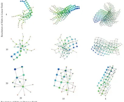
Fig. 5: Effects of Quantization. The bivariate functionf :IR3→IR2shown in Figure 1 was sampled onto a tetrahedral mesh, and the JCN was computed with slab intervals of 20, 10 and 4 with respect to both properties. Note that as the slab interval decreases, the JCN converges to the manifold structure of Figure 1, as predicted. Graph layout is still an issue, as appropriate aesthetics are as yet unclear. Here and elsewhere unless otherwise stated, force-directed layout has been used (vtkForceDirectedLayoutFilter). Each layout uses the same random seed for initial positioning of vertices, but final results are sensitive to graph structure and there is no guarantee of layout consistency between structurally similar graphs.

able geometric measures [9], topological simplification can be driven by geometric information, as with the Con-tour Tree and much of the existing literature on remesh-ing. We also note that this idea – of varying the level of simplification, was prefigured by Hilaga et al. [27] and Zhang et al. [46] in their computations of coarser versions of the Reeb Graph and Contour Tree.

We show the effects of varying levels of quantization in Figure 5 using a synthetic two-field dataset. One field has constant values along each row, decreasing from top to bottom. The second field approximates a radial distance function, with the origin at the center of the mesh. As expected, the combined fields exhibits a four-fold symmetry; the figure shows that the JCN captures this feature even at quite coarse resolutions.

This ability of the JCN to discriminate features at coarse levels has already been exploited to analyse data arising in a specific domain problem, identifying the point of “scission” within simulations of heavy

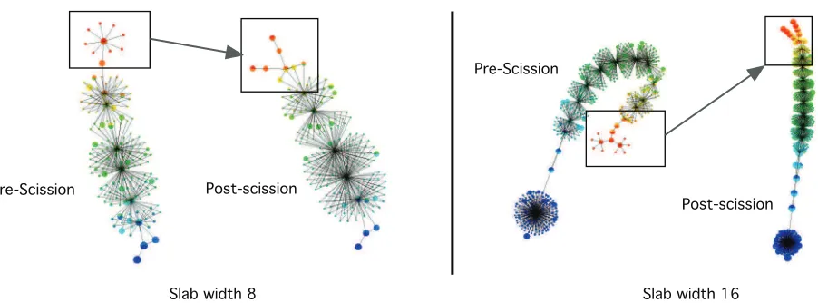
nu-clei [15], derived from density functional theory (DFT). Figure 6 uses four JCNs to show the joint topologi-cal structure of proton and neutron density fields for fermium. These JCNs were computed from volumetric density data in turn derived from two sites along a trajectory in the high-dimensional space underlying DFT. The data are 8-bit samples; the top row was constructed using a slab width of 32, the lower row a slab width of 16. Rectangles highlight the position of a significant combinatorial event, the point at which a nucleus split into multiple (in this case two) fragments.

Graph Layout: We have deliberately not considered

ab-Pre-Scission Post-scission

Slab width 16 Slab width 8

Pre-Scission

[image:11.612.55.506.48.215.2]

Post-scission

Fig. 6: Joint Contour Nets of nuclear density data used to locate the scission (nucleus fragmentation) point along a trajectory in a higher-dimensional space defined by density functional theory. JCN’s in the left column are pre-scission, those in the right are post-scission. Identification of combinatorial change in the JCN structure is marked by boxes. The top row is computed at slab width 16, the second row at slab width 8. Although the bottom-left figure shows some branching in the structure, the scission point is marked by the appearance of extended linear branches, a hypothesis supported by blind calibration experiments carried out by our physics collaborators [15].

straction for multifield topology, further work will be needed to map out structural properties of the network that should be highlighted in its external representation. There is clearly a “chicken and egg” problem here; we break the cycle by using force-directed layout in the first instance, on the grounds that there has been success in using the algorithms to highlight structural symmetry and other regularities in both local and global network structure. As recent work on layout of Contour Trees demonstrates [25], it can take signficant time and effort between identifying important abstractions, and having effective algorithms for their representation.

Summary: In short, many properties of the Contour

Tree that have been applied for visualization have direct equivalents in the JCN, and we can predict that this will allow the development of topological tools for multifield visualization. As an example of the use of the JCN to analyse multivariate data, Figure 6 shows illustrations from an application paper [15] applying JCN analysis for nuclear fission simulations. Figure 7 shows the JCN for a vector field from the meso-scale atmospheric simu-lation [26]: the resimu-lationship between the JCN (operating on arbitrary collections of scalar fields), and tools for the topological analysis of ‘multifields’ representing vector and tensor quantities, is an interesting but open question.

8

I

MPLEMENTATION

: B

ASE

A

LGORITHM

The JCN algorithm has been implemented as a filter for the Visualization Toolkit (VTK) [38]. As proof-of-concept, our initial implementation favours brute-force simplicity and generality over performance. The filter takes as input an unstructured grid, which is assumed to contain simplicial cells (either all triangles, or all tetrahedra), and generates three outputs:

1) the Joint Contour Net, as an undirected graph

2) (optionally) each individual fragment, as a polyg-onal mesh

3) (optionally) each contour slab, as a polygonal mesh Dataset processing goes through three phases. In the first, simplicial cells are converted into fragments. In-ternally we maintain a queue of (partially fragmented) polytopes (polygons or polyhedra, depending on dimen-sionality). We iterate over cells, initialising the fragment queue to the cell itself. Then for each scalar field and threshold, we run through the fragment queue, cutting each polytope against the current field threshold, and requeuing the resulting fragments. Once a polytope can-not be clipped further, it is placed in the output. Second, the dual graph of fragments is computed using tables from the first phase that record information about shared fragment edges/faces. The dual graph is then simplified by collapsing adjacent nodes with the same combination of field values. Last, Joint Contour Slab boundaries are computed by iterating over fragment facets (edges or faces) and discarding those internal to a slab.

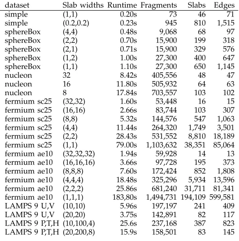
Testing has been carried out on both synthetic datasets (allowing for verification of the JCN implementation), and on the real fermium and plutonium datasets referred to in the application paper [15]. In the case of single-field data (e.g. the nucleon dataset), the JCN analysis shows that the JCN reduces to a tree, as expected. As a baseline for future work, Tables 1 and 2 set out the results of runtime tests. The former reports dataset sizes, while the latter gives performance measurements: the width (granularity) of each slab across each data dimension; the total number of fragments generated; the number of slabs; and the size of the resulting contour net.

[image:12.612.197.527.59.289.2] [image:12.612.313.564.362.482.2]

Fig. 7: Fields U and V (horizontal vector components) from time Step 11 of the Limited Area Meso-Scale Prediction System (LAMPS) data set [26]. In this example JCN nodes on the right are positioned in a 3D space at the barycenter of the corresponding slabs on the left. The circular structure in the JCN appears to correspond to rotational movement in the simulation: we expect to explore this further in future work.

TABLE 1: Dataset Statistics

Dataset Spatial Dimensions Simplices Field Widths

simple 3×3 8 9×9

sphereBox 11×6×11 2,500 [0,6]×[-4,71] nucleon 41×41×41 320,000 256 fermium 19×19×19 29,160 256×256×256

underlying field. For fermium, the trials reported involve doubling the resolution of three fields, so in the worst case we might expect an 8-fold increase in runtime and output size. Other than in the transition to (1,1,1), runtime growth is closer to a factor of 2, while changes in JCN node and edge size vary by around 5. These figures should be treated with caution, since our implementation was proof-of-concept rather than production-oriented. For example, it explicitly constructs and discards large volumes of fragment geometry.

9

R

ASTER

A

CCELERATION

As noted above, the effect of the JCN is to tessellate the function manifold with respect to the range of the function rather than the domain. Moreover, since the slabs are defined by intervals in each univariate channel in the range, the effect is to project a regular grid in the range onto the function manifold, with each Joint Contour Slab corresponding to a Euclidean box in the range. For a function f : IR2 → IR2, these boxes are pixels, and the relationship to Bachthaler & Weiskopf’s work on continuous scatterplots [2] becomes apparent.

Since the neighbourhood relationships of pixels are easily described, this simplifies the computation of the

8/7 7/8

4/4 5/5

5 6 7 8

4 5 6 7 8

4

Fig. 8: Rasterising the JCN. Each slab (left) corresponds to a Euclidean box (pixel) in the range (right), trans-forming this into a rasterisation problem. Each pixel rasterised corresponds to a fragment.

JCN by transforming it to a well understood rasterisation problem. For two dimensions, this immediately gives an effective method of computing the JCN without explic-itly extracting geometric slabs. This gives a full order of magnitude speed up compared with the na¨ıve algorithm, at a slight cost in accuracy because rasterisation algo-rithms do not necessarily rasterise every pixelintersected by the primitive. However, since the JCN is already an approximate computation, this is an acceptable cost in some circumstances, and does give the basis for further acceleration once efficient and accurate rasterisation al-gorithms are available in arbitrary dimensions.

Explicit geometry

Rasterized Approximation

Explicit geometry

Rasterized Approximation

Fermium sCF, pre-scission (site 25)

Fermium sCF, post-scission (site 26)

Sl

a

b

w

idt

h

1

6

Sl

a

b

w

idt

h

8

Sl

a

b

w

idt

h

[image:13.612.49.549.58.479.2]

4

Fig. 9: Comparison between explicit geometric construction of JCN, and rasterization for two different methods of inter-cell linking, both before (site 25) and after scission (site 26) in fermium sCF dataset [15]. Differences in the graph structure, particularly at slabwidth 4, are a result of the approximation in rasterization (visible by comparing graphs at high slabwidth), and compounded by sensitivity of force directed layout to graph structure.

scission point of a fermium nucleus, at which a single nucleus breaks into two fragments. Within each figure the top row shows the images generated using explicit geometric construction of JCN slabs, for three different levels of quantization (slab widths 16, 8, and 4). The bottom row shows the rasterised approximation, with major features clearly carrying over, but some artifacts in the form of isolated nodes. We have not included a qualitative comparison of the LAMPS data, as for this JCN the appropriate layout positions nodes at the barycenter of the corresponding geometric slab [15], and the raster implementation does not generate this data.

Dataset statistics and timing information are shown in Table 3, using the system configuration described in Table 2. For the nucleon data (which consists of a single scalar field), we note that the geometric and raster

im-plementations return the same (tree) structure, and that the performance gain from the raster implementation improves substantially as finer levels of quantization.

10

C

ONCLUSIONS AND

F

UTURE

W

ORK

[image:14.612.52.539.93.205.2]

TABLE 3: Runtime statistics for rasterization, for a subset of the 2D range datasets from 2. Statistics for explicit geometry have been copied over for ease of comparison. Rasterization results for lower-dimensional (1D) datasets are also shown. Speedup was computed by taking the ratio of the times stated.

Explicit Geometry Rasterization

Dataset Quantization nr-frags nr-nodes nr-edges time nr-frags nr-nodes nr-edges time Speedup Fermium sc25 16,16 83,744 163 307 2.75 104,619 157 280 0.59 4.7 Fermium sc25 8,8 144,576 547 1,063 5.32 142,451 268 497 1.01 5.3 Fermium sc25 4,4 264,320 1,749 3,501 11.44 266,817 917 1,769 2.16 5.3 Fermium sc25 2,2 531,552 8,810 18,189 28.43 547,360 2,755 5,536 6.61 4.3 Fermium sc25 1,1 1,103,632 38,351 85,064 79.00 1,193,128 9,042 18,216 24.72 3.2 LAMPS 9 (U,V) 10, 10 197,197 241 490 5.96 163,428 310 444 1.54 3.8

Nucleon 32 405,556 48 47 8.35 402,104 48 47 1.62 5.2

Nucleon 16 505,932 64 63 11.33 500,831 64 63 1.72 6.6

Nucleon 8 703,557 103 102 17.61 774,496 103 102 1.94 9.1

Nucleon 4 1,095,526 166 165 29.80 1,091,981 166 165 2.44 12.2

TABLE 2: Runtime Statistics. All timings were performed on a 2GHz MacBook Air with 8GB memory, running OSX 10.7.5, and using VTK 5.10 configured as a re-lease build: times are substantially lower than previously reported[15], which used a debug build. Fermium tim-ings in this table use site 25 of the sCF trajectory, and proton and neutron density fields (see [15] for details). To broaden the results, a further set of timings has been included from a different trajectory from the same dataset, site aEF. This uses a third, derived, field (total density) that was not required for the study reported in [15]. LAMPS timings are for time step 9 of the dataset.

dataset Slab widths Runtime Fragments Slabs Edges

simple (1,1) 0.20s 73 46 71

simple (0.2,0.2) 0.23s 945 810 1,515 sphereBox (4,4) 0.48s 9,068 68 97 sphereBox (2,2) 0.70s 15,900 199 318 sphereBox (2,1) 0.71s 15,900 329 576 sphereBox (1,2) 1.00s 27,300 400 647 sphereBox (1,1) 1.10s 27,300 650 1,145 nucleon 32 8.42s 405,556 48 47 nucleon 16 11.80s 505,932 64 63 nucleon 8 17.84s 703,557 103 102 fermium sc25 (32,32) 1.60s 53,448 16 15 fermium sc25 (16,16) 2.66s 83,744 103 307 fermium sc25 (8,8) 5.32s 144,576 547 1,063 fermium sc25 (4,4) 11.44s 264,320 1,749 3,501 fermium sc25 (2,2) 28.43s 531,552 8,810 18,189 fermium sc25 (1,1) 79.00s 1,103,632 38,351 85,064 fermium ae10 (32,32,32) 1.94s 59,928 14 13 fermium ae10 (16,16,16) 3.66s 97,728 195 373 fermium ae10 (8,8,8) 7.60s 172,424 852 1,808 fermium ae10 (4,4,4) 18.48s 325,296 5,934 13,596 fermium ae10 (2,2,2) 25.86s 681,240 31,711 81,341 fermium ae10 (1,1,1) 183,80s 1,494,731 194,109 599,581 LAMPS 9 U,V (10,10) 5.96s 197,197 241 409 LAMPS 9 U,V (20,20) 3.75s 142,891 82 117 LAMPS 9 P,T,H (10,100,4) 25.6s 237,168 387 823 LAMPS 9 P,T,H (20,200,8) 15.9s 158,501 83 145

the graph of the function, extracting and storing a fully meshed complex [4] will be useful for some problems, but that for other problems, such as parameter space analysis, construction from graph structures such as the Gabriel graph [11] will be more fruitful.

We also intend to study the relationship between the JCN and Jacobi Sets, and consider whether there is an equivalent to the Morse-Smale Complex. While the current work has used existing two-dimensional

rasterisation methods, future work will necessarily ex-tend to higher-dimensional rasterisation, which will be applicable not only to the JCN, but also to many other multi-variate analysis and visualisation techniques.

A

CKNOWLEDGEMENTS

Acknowledgements are due to Bob Laramee and Eugene Zhang, presentation of whose work triggered this line of thought. Our initial results on the nuclear fission datasets were produced in collaboration with Aaron Knoll, Nico-las Schunck, Hai Ah Nam, and Andrzej Staszczak. This work is supported by the UK Engineering and Physical Sciences Research Council under Grant EP/J013072/1. Thanks are also due to the anonymous reviewers for suggestions on how to improve the presentation and for the significant observation that the JCN re-tessellates the graph of the function with respect to the range.

R

EFERENCES

[1] M. Allili, M. Ethier, and T. Kaczynski. Critical Region Analysis of Scalar Fields in Arbitrary Dimensions. InProceedings of Visual-ization and Data Analysis 2010, pages 753008–12, 2010.

[2] S. Bachthaler and D. Weiskopf. Continuous Scatterplots. IEEE Transactions on Visualization and Computer Graphics, 14(6):1428– 1435, 2008.

[3] R. L. Boyell and H. Ruston. Hybrid Techniques for Real-time Radar Simulation. InProceedings, 1963 Fall Joint Computer Confer-ence, pages 445–458. IEEE, 1963.

[4] D. Canino, L. de Floriani, and K. Weiss. IA*: An Adjacency-Based Representation for Non-Manifold Simplices in Arbitrary Dimensions. Computers and Graphics, 35(3):747–753, 2011. [5] G. Carlsson, G. Singh, and A. Zomorodian. Computing

Multi-dimensional Persistence. Journal of Comp. Geometry, 1(1):72–100, 2010.

[6] H. Carr, B. Duffy, and B. Denby. On Histograms and Isosurface Statistics.IEEE Transactions on Visualization and Computer Graphics, 12(5):1259–1266, September/October 2006.

[7] H. Carr and J. Snoeyink. Representing Interpolant Topology for Contour Tree Computation. In H.-C. Hege, K. Polthier, and G. Scheuermann, editors, Topology-Based Methods in Visualization II, Mathematics and Visualization, pages 59–74. Springer, 2009. [8] H. Carr, J. Snoeyink, and U. Axen. Computing Contour Trees in

All Dimensions. Computational Geometry: Theory and Applications, 24(2):75–94, 2003.

[image:14.612.50.296.372.620.2]

[10] Y.-J. Chiang, T. Lenz, X. Lu, and G. Rote. Simple and Optimal Output-Sensitive Construction of Contour Trees Using Monotone Paths.Computational Geometry: Theory and Applications, 30:165–195, 2005.

[11] C. D. Correa and P. Lindstrom. Towards Robust Topology of Sparsely Sampled Data. IEEE Transactions on Visualization and Computer Graphics, 17(12):1852–1861, 2011.

[12] H. Doraiswamy and V. Natarajan. Computing Reeb Graphs as a Union of Contour Trees. IEEE Transactions on Visualization and Computer Graphics, page DOI: 10.1109/TVCG.2012.115, 2012. [13] B. Duffy and H. Carr. Interval based data structure optimisation.

InProceedings, Theory and Practice of Computer Graphics 2010, pages 151–158, 2010.

[14] B. Duffy, H. Carr, and T. M ¨oller. Integrating Histograms and Iso-surface Statistics. IEEE Transactions on Visualization and Computer Graphics, 19(2):263–77, 2013. DOI: 10.1109/TVCG.2012.118. [15] D. Duke, H. Carr, A. Knoll, N. Schunck, H. A. Nam, and

A. Staszczak. Visualizing nuclear scission through a multifield extension of topological analysis.IEEE Transactions on Visualization and Computer Graphics, 18(12):2033–40, 2012.

[16] H. Edelsbrunner.Algorithms in Combinatorial Geometry. Springer-Verlag, 1987.

[17] H. Edelsbrunner and J. Harer. Jacobi Sets of Multiple Morse Functions. InFoundations in Computational Mathematics, pages 37– 57, Cambridge, U.K., 2002. Cambridge University Press. [18] H. Edelsbrunner, J. Harer, A. Mascarenhas, V. Pascucci, and

J. Snoeyink. Time-Varying Reeb Graphs for Continuous Space-Time Data.Computational Geometry, 41(3):149–166, 2008. [19] H. Edelsbrunner, J. Harer, and A. K. Patel. Reeb Spaces of

Piecewise Linear Mappings. In Proceedings of ACM Symposium on Computational Geometry, pages 242–250., 2008.

[20] H. Edelsbrunner, J. Harer, and A. Zomorodian. Hierarchical Morse Complexes for Piecewise Linear 2-Manifolds. In Proceed-ings, 17th ACM Symposium on Computational Geometry, pages 70– 79. ACM, 2001.

[21] H. Edelsbrunner and E. P. M ¨ucke. Simulation of Simplicity: A Technique to Cope with Degenerate Cases in Geometric Algo-rithms.ACM Transactions on Graphics, 9(1):66–104, 1990. [22] R. Forman. Discrete Morse Theory for Cell Complexes.Advances

in Mathematics, 134:90–145, 1998.

[23] W. Harvey and Y. Wang. Generating and Exploring a Collec-tion of Topological Landscapes for VisualizaCollec-tion of Scalar-Valued Functions.Computer Graphics Forum, 29(3), 2010.

[24] W. Harvey, Y. Wang, and R. Wenger. A Randomized O(m log m) Algorithm for Computing Reeb Graphs of Arbitrary Simplicial Complexes. InACM Symposium on Computational Geometry, pages 267–276, 2010.

[25] C. Heine, D. Schneider, H. Carr, and G. Scheuermann. Drawing contour trees in the plane. IEEE Transactions on Visualization and Computer Graphics, 17(11):1599–1611, 2011.

[26] W. Hibbard and D. Santek. Visualizing Large Data Sets in the Earth Sciences.Computer, 22(8):53–57, 1989.

[27] M. Hilaga, Y. Shinagawa, T. Kohmura, and T. L. Kunii. Topology Matching for Fully Automatic Similarity Estimation of 3D Shapes.

ACM Transactions on Graphics, pages 203–212, 2001.

[28] S. Maadasamy, H. Doraiswamy, and V. Natarajan. A hybrid parallel algorithm for computing and tracking level set topology. In High Performance Computing (HiPC), 2012 19th International Conference on, pages 1–10. IEEE, 2012.

[29] D. Morozov and G. Weber. Distributed merge trees. InProceedings of the 18th ACM SIGPLAN symposium on Principles and practice of parallel programming, PPoPP ’13, pages 93–102, New York, NY, USA, 2013. ACM.

[30] S. Nagaraj and V. Natarajan. Simplification of Jacobi Sets. In V. Pascucci, X. Tricoche, H. Hagen, and J. Tierny, editors, Topo-logical Data Analysis and Visualization: Theory, Algorithms and Ap-plications, Mathematics and Visualization, pages 91–102. Springer, 2011.

[31] S. Parsa. A Deterministic O(m log m) Time Algorithm for the Reeb Graph. InACM Symposium on Computational Geometry, pages 269–276, 2012.

[32] V. Pascucci and K. Cole-McLaughlin. Parallel Computation of the Topology of Level Sets.Algorithmica, 38(2):249–268, 2003. [33] V. Pascucci, G. Scorzelli, P.-T. Bremer, and A. Mascarenhas. Robust

On-line Computation of Reeb Graphs: Simplicity and Speed.ACM Transactions on Graphics, 26(3):58.1–58.9, 2007.

[34] G. Reeb. Sur les Points Singuliers d’une Forme de Pfaff Compl`etement Int´egrable ou d’une Fonction Num´erique.Comptes Rendus de l’Acad`emie des Sciences de Paris, 222:847–849, 1946. [35] O. Saeki.Topology of Singular Fibers of Differentiable Maps. Number

1854 in Lecture Notes in Mathematics. Springer, 2004.

[36] C. E. Scheidegger, J. M. Schreiner, B. Duffy, H. Carr, and C. T. Silva. Revisiting Histograms and Isosurface Statistics. IEEE Transactions on Visualization and Computer Graphics, 14(6):1659–1666, 2008. [37] D. Schneider, A. Wiebel, H. Carr, M. Hlawitschka, and G.

Scheuer-mann. Interactive Comparison of Scalar Fields Based on Largest Contours with Applications to Flow Visualization. IEEE Transac-tions on Visualization and Computer Graphics, 14(6):1475–1482, 2008. [38] W. Schroeder, K. Martin, and B. Lorensen.The Visualization Toolkit: An Object-Oriented Approach to 3D Graphics. Kitware, Inc., fourth edition, 2006.

[39] R. E. Tarjan. Efficiency of a Good but not Linear Set Union Algorithm.Journal of the ACM, 22:215–225, 1975.

[40] J. Tierny, A. Gyulassy, E. Simon, and V. Pascucci. Loop Surgery for Volumetric Meshes: Reeb Graphs Reduced to Contour Trees.IEEE Transactions on Visualization and Computer Graphics, 15(6):1177– 1184, 2010.

[41] M. van Kreveld, R. van Oostrum, C. L. Bajaj, V. Pascucci, and D. R. Schikore. Contour Trees and Small Seed Sets for Isosurface Traversal. In Proceedings, 13th ACM Symposium on Computational Geometry, pages 212–220, 1997.

[42] M. J. van Kreveld, R. van Oostrum, C. L. Bajaj, V. Pascucci, and D. R. Schikore. Topological Data Structures for Surfaces: An Introduction for Geographical Information Science, chapter 5: Efficient contour tree and minimum seed set construction, pages 71–86. John Wiley & Sons, May 2004.

[43] G. Weber, P.-T. Bremer, and V. Pascucci. Topological Land-scapes: A Terrain Metaphor for Scientific Data. IEEE Transactions on Visualization and Computer Graphics, 13(6):1416–1423, Novem-ber/December 2007.

[44] G. Weber, S. Dillard, H. Carr, V. Pascucci, and B. Hamann. Topology-Controlled Volume Rendering. IEEE Transactions on Visualization and Computer Graphics, 13(2):330–341, March/April 2007.

[45] G. Weber, G. Scheuermann, and H. Hagen. Detecting Critical Regions in Scalar Fields. In Proceedings of Eurographics-IEEE Symposium on Visualization 2003, pages 85–94,288, 2003.

[46] X. Zhang, C. L. Bajaj, and N. Baker. Fast Matching of Volumetric Functions Using Multi-resolution Dual Contour Trees. Technical report, Texas Institute for Computational and Applied Mathemat-ics, Austin, Texas, 2004.

Hamish Carr completed his PhD at the Uni-versity of British Columbia in May 2004 and has worked as a lecturer at University College Dublin and a senior lecturer at the University of Leeds. His research interests include scientific and medical visualization, computational geom-etry and topology, computer graphics and geo-metric applications. He is a member of the IEEE and the IEEE Computer Society and Chair of the UK Chapter of the Eurographics Association.