A rectangular waveguide cell for measurement of the shielding effectiveness of anisotropic materials

This is a repository copy of

A rectangular waveguide cell for measurement of the shielding

effectiveness of anisotropic materials

.

White Rose Research Online URL for this paper:

http://eprints.whiterose.ac.uk/132796/

Version: Published Version

Proceedings Paper:

Flintoft, Ian David orcid.org/0000-0003-3153-8447, Marvin, A C

orcid.org/0000-0003-2590-5335, Dawson, J F orcid.org/0000-0003-4537-9977 et al. (1

more author) (2010) A rectangular waveguide cell for measurement of the shielding

effectiveness of anisotropic materials. In: EMC Europe 2010, 9th International Symposium

on EMC joint with 20th International Wroclaw Symposium on EMC:13-17 September,

2010. Oficyna Wydawnicza Politechniki Wroclawskiej , Wroclaw, Poland , pp. 591-596.

[email protected] https://eprints.whiterose.ac.uk/ Reuse

Items deposited in White Rose Research Online are protected by copyright, with all rights reserved unless indicated otherwise. They may be downloaded and/or printed for private study, or other acts as permitted by national copyright laws. The publisher or other rights holders may allow further reproduction and re-use of the full text version. This is indicated by the licence information on the White Rose Research Online record for the item.

Takedown

If you consider content in White Rose Research Online to be in breach of UK law, please notify us by

A Rectangular Waveguide Cell for Measurement of

the Shielding Effectiveness of Anisotropic Materials

L. Dawson, I.D. Flintoft, A.C. Marvin and J.F. Dawson

Department of Electronics University of York, Heslington,

York, UK, YO10 5DD {ld5,idf1,acm,jfd}@ohm.york.ac.uk

Abstract— A method for measuring the shielding effectiveness of planar anisotropic materials using a rectangular waveguide cell is proposed. Computational models are used to verify the behaviour of the cell and validate its ability to measure shielding effectiveness. Results of measurements on a control sample and three carbon-fibre composite laminates in a GTEM cell are presented. A dynamic range of 70 dB with a capability to discriminate 20 dB of anisotropy is achieved in the frequency range 400-1600 MHz using cubic cells of side length 200 mm and 300 mm.

Keywords: shielding measurement, shielding effectiveness, composite materials, anisotropic materials

I. INTRODUCTION

When constructing enclosures to have a particular level of shielding it is necessary to know the properties of the material from which the enclosure is to be manufactured. Most materials traditionally used for this purpose are isotropic in their shielding performance, but with the increasing use of carbon-fibre composite (CFC) materials that are built up from layers of fibres that are layered in different directions, or woven in different ways, this is no longer the case.

Knowledge of the differing shielding performance with polarisation of the incident electromagnetic field is therefore important as design criteria for the enclosure. Also, when considering the overall electromagnetic compatibility of complex systems, such as aircraft exposed to external High Intensity Radiated Field (HIRF) threats, it is increasingly important to have an accurate model for the shielding characteristics of the composite materials used in the construction of the system. It is difficult to derive these models directly from known characteristics of the composite; hence an experimental technique that allows macro-models to be derived from measurements of the actual materials used is being sought [1]. Unfortunately many of the standard methods generally used to measure the shielding effectiveness (SE) of planar samples provide a result that is determined by the overall performance of the material, with the polarisation effects „averaged‟ out [2]. The coaxial ASTM cell, used at lower frequencies, illuminates the sample with a radially polarised electric field [3]. The nested reverberation chamber

technique applies a statistical field to the sample consisting of illumination from all polarisations and angles of incidence [4,5]. Both these techniques yield a SE that is a dominated by the lowest shielding polarisation direction of the material. Other techniques based on wide band horns have been considered [6].

In this paper we describe the initial developments of a measurement technique based on a waveguide cell that has some capability to measure the polarisation dependence of the SE of planar anisotropic samples. The rationale of the proposed method is described in Section II. A number of computational models that were used to develop the technique are described in Section III. Section IV presents the results of a series of measurements made on CFC samples using cells of two sizes. Section V summarises the paper and indicates further work being undertaken.

II. THE PROPOSED METHOD

The proposed method uses a rectangular waveguide cell with a square cross-section as shown schematically in Fig. 1.

The “front” face of the cell contains a large aperture over

which the sample is fixed. Inside the cavity formed by the cell and sample a probe antenna is used to sense the electric field immediately behind the sample. The sample is then illuminated externally with a linearly polarised uniform plane electromagnetic wave using a suitable transducer, for example a standard antenna in an anechoic chamber (AC) or a Gigahertz Transverse Electromagnetic (GTEM) cell. The internal probe antenna is a balanced dipole that is aligned with the polarisation of the illuminating field. The SE of a sample for a given polarisation of the incident field can then be determined by an insertion loss measurement on the transmission through the system. The response for the perpendicular polarisation is obtained by turning the sample though 90 degrees. The ability to discriminate anisotropy will depend on a number of factors including the polarisation purity of the external transducer, the characteristics of the modes excited inside the cell and the balance of the dipole. These factors are discussed and investigated below.

the region of the TE10 propagation. The small balanced dipole was supported using a length of semi-rigid coaxial cable attached via a SMA connector at the centre of the rear face. The addition of the cable meant that the system was no longer a simple waveguide operating below cut-off or with a small number of propagating modes, but also had a TEM mode of propagation. Ideally an optically coupled probe would have been used but the dimensions of the system and the sensitivity required meant that this was not possible. Radio absorbing material (RAM), either layered foam or ferrite tiles, was placed at the rear of the cell to terminate any propagating modes [7].

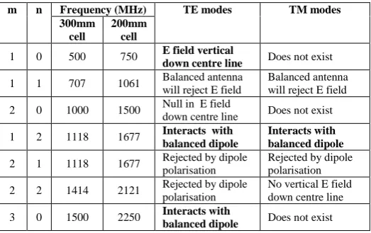
Examination of the field patterns of the first few propagating modes in the cell shows that a well-balanced dipole positioned in the centre of the face will reject several of the lowest frequency modes due to a number of factors: (1) The balance of the dipole rejecting coaxial like modes. Importantly this is the case for the TEM mode caused by the cable to the probe antenna; (2) The polarisation of the waveguide mode being normal to the dipole polarisation; (3) The waveguide mode has a null in the vertical electric field at the position of the dipole. These effects and the corresponding cut-off frequencies for cells with side lengths of 200mm and 300mm are summarised in Table 1.

TABLE I. SUMMARY OF THE LOWEST FREQUENCY WAVEGUIDE TEmn

AND TMmn MODES IN THE 200 MM AND 300 MM CELLS AND HOW THEY

INTERACT WITH A BALANCED DIPOLE SENSOR AT THE CENTRE OF THE CELL.

m n Frequency (MHz) TE modes TM modes 300mm

cell

200mm cell

1 0 500 750 E field vertical

down centre line Does not exist

1 1 707 1061 Balanced antenna will reject E field

Balanced antenna will reject E field

2 0 1000 1500 Null in E field

down centre line Does not exist

1 2 1118 1677 Interacts with

balanced dipole

Interacts with balanced dipole

2 1 1118 1677 Rejected by dipole polarisation

Rejected by dipole polarisation

2 2 1414 2121 Rejected by dipole polarisation

No vertical E field down centre line

3 0 1500 2250 Interacts with

balanced dipole Does not exist

The first higher order mode which will interact with the balanced dipole is the degenerate TE/TM21 and TE/TM12, at a frequency of 1118 MHz in a 300 mm cell and 1677 MHz in a 200 mm cell. This mode will also couple horizontally to vertically polarised fields and therefore defines the upper frequency limit of the use of each cell when measuring anisotropic samples. In practice achieving good rejection of the TE/TM11 and TE20 is difficult since it requires very good physical and electrical balance from the dipole antenna and high symmetry and homogeneity of the cell and sample.

Three enclosures were manufactured from brass plate as shown in Fig. 2. They were all cubic with dimensions of 100mm, 200mm and 300mm with TE10 mode cut-off

frequencies of 500MHz, 750MHz and 1500MHz respectively. The sample holder consists of a flange on the front face of the cell with a conductive gasket inset. The sample is trimmed to overlap the gasket and then clamped in place using another brass plate and brass bolts. As usual with shielding measurements, obtaining good electrical contact with the sample is imperative to achieving reliable measurements [8].

III. ANALYSIS OF THE TEST CELL

A. Method-of-Moments Simulation of Dipole Balance The 200mm cell was modelled using a method-of-moments (MoM) solver to investigate the effects of the balance of the probe antenna on the response of the system [9]. The computational mesh of the MoM model is shown in Fig. 3. The cell walls were modelled using perfectly conducting boundaries with a basic patch size of 10 mm and local refinement near the edges of the aperture, cell corners and the attachment point of the cable to the dipole probe. The arms of the dipole were modelled using a wire with two 25  resistive loads either side of the central segment, to which another wire representing the outer shield of the coaxial cable was attached. This allowed the overall 50 impedance of the cable to be modelled and both the balanced and unbalanced response of the dipole to both the waveguide TE10 and coaxial TEM modes to be calculated from the phasor sum and difference of Figure 2. Photograph of the 100 mm and 200 mm test cells showing the sample mounting plate with conductive gasket and probe dipole.

Front plate clamping sample to cell

Conductive gasket Balanced dipole

with balun

Absorber (carbon loaded or ferrite)

Sample under test

10mm

the voltages in the two loads respectively. To represent the imperfect balance of a physical dipole the length of the arms of the modelled dipole could be made unequal.

The front face of the cell was illuminated by a uniform plane wave polarised in the z-direction, co-polar to the dipole. The results are presented as a reception aperture, Arec, defined

by

inc rec rec

S

P

A



where Prec is the power received in the dipole load and Sinc is

the power density of the field incident on the sample.

Fig. 4 shows the results of the MoM model when the dipole is not perfectly balanced (one arm was made 5 mm longer than the other). Note that for this model there was no absorber on the back wall of the enclosure as this could not be modelled efficiently using the MoM code. The intended balanced response of the dipole to the illuminating plane-wave exhibits a smooth response over the whole frequency range depicted. The unbalanced response to the coaxial TEM mode along the cable is typically 10 to 20 dB lower then the balanced response, except near 330 MHz where the cable, “top-loaded” by the dipole, is an open circuit quarter-wave transmission-line. Here there is a substantial response from the imbalanced dipole, demonstrating the importance of maximising the dipole balance in the physical system.

Fig. 4 also shows measurement results obtained by illuminating the cell with a log-periodic antenna in an AC. Results are shown for a completely unloaded cell and for the case where the back wall of the cell is loaded with ferrite

absorber. The unloaded measurement is in good agreement with the predicted balanced response of the MoM model. The peak in the unloaded measurement at 330 MHz, caused by the quarter-wave resonance of the TEM mode on the cable, is in reasonable agreement with the unbalanced response predicted by the model. Loading the cell with ferrite can be seen to substantially reduce the effect of this resonance, mitigating the imperfect balance of the physical dipole antenna.

The cross-polar response of the dipole antenna in the illuminating transducer will limit the ability of the cell to discriminate anisotropic samples. Fig. 5 shows the measured co- and cross-polar response of the 200 mm cell without a sample, illuminated by a log-periodic antenna in an AC. In these measurements the cell was again either completely unloaded or had ferrite tiles on the rear wall. The results show that the polarisation purity of this system was limited to about 15dB. For this configuration the limiting factor was found to be the log-periodic antenna in which the staggered design of the elements causes a significant cross-polar field.

Figure 5. Co-polar and cross-polar coupling of the 200 mm cell wthout a sample measured in an anechoic chamber with and without ferrite absorber on back wall of the cell.

Figure 3. The method-of-moments model of the 200mm cell. The model does not include absorbing material at the back of the cell . Points 1 and 2 are the location of the two 25  loads used to calcalute the differential-mode and common-differential-mode responses.

B. Transmission-Line Matrix Model of SE Measurement

The capability of the test cell to determine the SE of a sample was also investigated using a Transmission Line Matrix (TLM) model of the 300mm cell [10]. The geometry of the model is shown in Fig. 6. The cell was modelled as a cubic perfect electrically conducting (PEC) box with the upper face left open; the flange was not included for simplicity. The rear of the cell was loaded with a model of multilayered carbon-loaded foam RAM using material parameters from the manufacture‟s datasheet [6]. Due to limitations of the TLM code only a frequency independent material could be modelled, so the parameters at 1 GHz were used. The dipole was modelled using a line of PEC cells with a split load across another line of PEC cells representing the cable, similar to the MoM discussed earlier. A uniform Cartesian mesh was used with a cell size of 5 mm. The overall size of the model was 1203 cells occupying about 120 Mb and requiring a run-time of about 60 minutes.

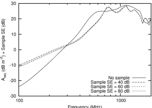
Verification that the system was indeed measuring SE was obtained by modelling samples with different characteristics using a sub-cell partially reflecting/transmitting TLM boundary with defined transmission coefficients [10]. This boundary was defined across the whole upper face of the cell in Fig. 6. These boundaries are the TLM equivalent of impedance boundary models in finite-difference time-domain, which are often used to simulate composite materials [11,12,13]. The TLM boundary model is parameterised by the scattering matrix of the transverse field components at the boundary. To show more explicitly the abilities and dynamic range of the system a range

of “fictitious” numerical samples with frequency independent transmission coefficients ranging from -40 dB to -80 dB were modelled (the corresponding reflection coefficient, was chosen to ensure energy conservation and provide a little absorption in the boundary). The transmission coefficient defined for the boundary is implicitly the inverse of the plane-wave infinite

planar SE of the “fictitious” sample.

The results of the TLM simulations are shown in Fig. 7 as the reception aperture of the cell in dB m2, defined in (1), plus the known plane wave SE of the numerical sample in dB. The reception aperture for the cell with no sample is also shown. If the change in response of the cell with a sample is purely due to the SE of the sample all the curves should overlay. The close agreement between the curves for all the high shielding samples implies that the difference in reception aperture of the

cell with different samples is predominantly due to the SE of the sample. However, the substantial difference between the curves with a sample and without a sample (which is often used as the calibration method) indicates that the difference in reception aperture relative to the no sample case is not purely due the SE of material. The above results imply that the cell can be used to measure SE but that the calibration of the system is not as simple as comparing the transmission through the system with (S21sample) and without (S21nosample) the sample

and defining the SE as the ratio

sample 21 nosample 21 sample

S

S

SE



Instead, it is necessary to calibrate the system using a reference sample with similar reflectivity to the sample-under-test, so that the mode structure in the cell is the same in both measurements. Providing the SE of the reference sample (which does not need to be anisotropic) is already known, the SE of the sample-under-test can be defined using

sample 21

ref 21 ref sample

S

S

SE

SE



where SEref is the known SE of the reference sample, SE21ref is

the measured transmission through the reference sample and SE21sample is the measured transmission through the

sample-under-test. Well controlled reference samples with suitable characteristic can be easily be manufactured, for example, from metal plates with a periodic two-dimensional array of small circular apertures. Such perforated plates have a 20 dB/decade behaviour at low frequencies and they can be measured reliably using other techniques [3,4,5].

The results in Fig. 7 also show that the reception aperture with a sample in place falls at 20 dB/decade with decreasing frequency below 300 MHz, limiting the dynamic range of the system at low frequency. However, many samples of interest, including CFCs, have lower SE at low frequencies so this behaviour matches that of the sample.

Figure 6. Illustration of the TLM model of the 300 mm cell with layered absorber on the back of the cell. Note that the flange is not included on the front face of the cell. The cell is illuminated from the upper side of the grid using a Huygen‟s surface.

IV. GTEMSAMPLE MEASUREMENTS

Measurements on a number of samples were undertaken using the 200 mm and 300 mm waveguide cells in a GTEM cell. The GTEM was expected to have greater polarisation purity and uniformity than the log-periodic antenna used in the AC and therefore provide greater discrimination of sample anisotropy. The experimental configuration used is shown in Fig. 8. In order to increase the dynamic range of the measurement to a level suitable for CFC samples a power amplifier was used to increase power of the illuminating field. A calibrated variable attenuator was then used to control the transmit power depending on the SE of the sample in order to protect the network analyser.

The cross polar field in the 300 mm cell was measured by turning the cell through 90 degrees and is shown in Fig. 9. Over the operational range of the cell the cross-polar response is seen to be approximately 20 dB below the co-polar fields. This is a 5 dB improvement compared to using the same cell in an AC with a log-periodic antenna. These measurements indicate that any anisotropy which causes a difference in the SE between the two polarisations of greater than 20 dB cannot be measured.

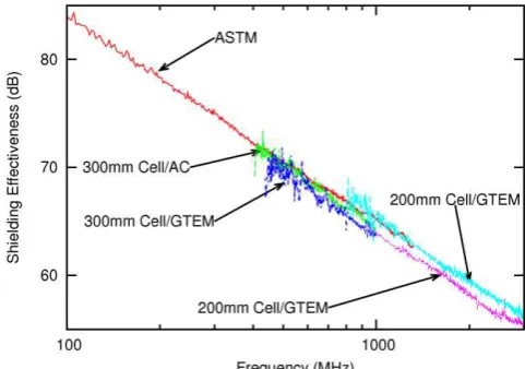
The cells were calibrated using a perforated brass sheet, 0.3mm in thickness, with a periodic array of 3 mm diameter holes spaced on a two-dimensional 10 mm grid. This reference sample was also measured in an ASTM cell and a straight line fit to the SE (in dB) as a function of frequency was obtained for use in (3).

An initial measurement was then made on another perforated plate with a grid of 1.5 mm diameter holes spaced at 5 mm. This plate has an SE about 6 dB higher than the reference sample and was also measured in the ASTM cell. Fig. 10 shows the SE of this plate measured in the 200mm and 300 mm test cells compared to the ASTM measurement. Note that the two measurements for the 300 mm cell in the GTEM use different power amplifiers. The agreement between the test cells and the standard ASTM method is seen to be very good for this metallic isotropic sample, typically lying within about 1 dB of each other. This shows that for an isotropic sample the technique described here can give results that are very similar to those obtained from the ASTM cell. This can be an advantage as the authors have found that the ASTM cell is very fragile and is prone to error if the centre conductors do not meet correctly. Note that the measurement is in fact also accurate above the nominal cut-off frequency of the 200 mm cell at about 1.6 GHz.

Further measurements were then made on a series of three CFC samples. Sample 1 (CFC1) consisted of a single layer of 5-harness satin weave which was physically unbalanced and tended to bend unless it was restrained. Sample 2 (CFC2) was a twin layer of the same 5-harness satin weave constructed in such a way that the laminate was mechanically balanced and remains flat unless force is applied. The structure of sample 3 (CFC3) is unknown, although it is a commercial aerospace laminate. All three samples were encased in resin giving a flexible sheet of thickness 0.5 mm (CFC1 and CFC3) and 0.65 mm (CFC2).

As with most SE measurements the results depend on the sample edge preparation (a good electrical contact must be formed around the whole sample) and each sample was

Network analyser Septum

Probe

Amplifier

attenuator

Figure 8. Measurement set-up in the GTEM cell.

Figure 9. Measurement of the transmission (S21) between the GTEM and the 300 mm cell with no sample in co-polar and cross-polar configurations.

prepared by abrading the edges and surface near the edge before applying a coat of conductive paint around the side and over the abraded surface so that it would meet with the surface of the conducting gasket which can be observed in Fig. 2.

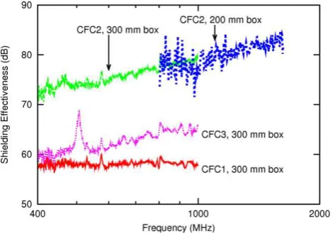
The measured SEs of the three CFC samples in two orthogonal polarisations are shown in Fig. 11 and Fig. 12. The

terms „vertical‟ and „horizontal‟ refer to a nominal reference

direction marked on each sample relative to the weave of the fibres. It can be seen that the results from the two enclosures overlap well but that there is a potential problem with sensitivity in the smaller enclosure for the samples with higher screening. The results show that CFC1 and CFC3 have little anisotropy but that CFC2 shows anisotropy of approximately 6 dB which is well within the levels which can be accepted as due to the material not imperfections in the source.

V. CONCLUSIONS

The modelling and measurement results indicate that the waveguide test cells can be used to measure the shielding effectiveness of conducting materials providing the system is calibrated using a conducting sample with known shielding

effectiveness. Initial measurements indicate that the results for anisotropic materials are comparable to those obtained from an ASTM cell but further work needs to be carried out to compare with other techniques. The cell can be used to give an indication of anisotropy of materials but the difference, which can be obtained for the two polarisations, is limited to less than 20 dB. The frequency range of the cells is relatively limited as the maximum frequency which can be used for each cell is 2.1 times the cut-off frequency of the TE10 mode. Another major drawback, shared by most other techniques, is that the samples must be in good electrical contact with the enclosure which can be a problem for CFC and some other materials.

Further work is being undertaken to correlate the SE determined by the cells with other techniques such as nested reverberation chambers and an absorber system that can also discriminate anisotropy and to verify the polarization and anisotropic capabilities of the cell [14].

REFERENCES

[1] I. D. Flintoft, J. F. Dawson, A. C. Marvin and S. J. Porter, “Development of Time-Domain Surface Macro-Models from Material Measurements”, 23rd _{International Review of Progress in Applied}

Computational Electromagnetics (ACES2007), Verona, Italy, 19-23 March, 2007.

[2] P. F. Wilson, M. T. Ma and J. W. Adams, “Techniques for Measuring the Electromagnetic Shielding Effectiveness of Materials: Part I: - Far-Field Source Simulation”, IEEE Trans. Electromag. Compat., vol. 30, no. 3, pp. 239-249, Aug. 1988.

[3] American Society for Testing and Materials, “Standard test method for measuring the electromagnetic shielding effectiveness of planar materials”, Standard D4935-99, 1999.

[4] International Electrotechnical Commission, “Testing and measurement techniques - reverberation chamber test methods”, Standard 6100-4-21:2003, 2003.

[5] C. L. Holloway, D. A. Hill, J. Ladbury, G. Koepke, and R. Garzia, “Shielding effectiveness measurements of materials using nested reverberation chambers”, IEEE Trans. Electromag. Compat., vol. 45, no. 2, pp. 350–356, May 2003.

[6] J. Catrysse, “Shielding effectiveness of flat samples and conductive gaskets: New measuring cell for the frequency range 1-18 GHz”, IEEE Int. Symp. on Electromag. Compat., Detroit, 18-22 Aug., 2008. [7] Emerson and Cuming Microwave Products, ECCOSORB AN79

Material Data Sheet. Available: http://www.eccosorb.com.

[8] J. Catrysse, M. Delesie and W. Steenbakkers, “The influence of the test fixture on shielding effectiveness measurements”, IEEE Trans. Electromag. Compat., vol. 34, no. 3, pp. 348-351, Aug. 1999.

[9] H. D. Brüns, A. Freiberg and H. Singer, “CONCEPTII - Manual of the program system”, The Institute of Electromagnetic Theory, Department of Electrical Engineering, University of Technology Hamburg-Harburg. [10] C. Christopoulos, “The Transmission-Line Modeling (TLM) Method in

Electromagnetics”, Morgan & Claypool, 2006.

[11] J. F. Dawson, “Representing ferrite absorbing tiles as frequency dependent boundaries in TLM”, IEE Electronics Lett., vol. 29, no. 9, pp. 791-792, Sep. 1993.

[12] M. S. Sarto, "A new model for the FDTD analysis of the shielding performances of thin composite structures", IEEE Trans. Electromag. Compat., vol. 41, no..4, pp. 298-306, Nov. 1999.

[13] C. L. Holloway, M. S. Sarto and M. Johansson, “Analyzing Carbon -Fiber Composite Materials With Equivalent-Layer Models”, IEEE Trans. Electromag. Compat., vol. 47, no. 4, pp. 833-844, Nov. 2005. [14] A. C. Marvin, L. Dawson and I. D. Flintoft and J. F. Dawson, “A

Method for the Measurement of Shielding Effectiveness of Planar Samples Requiring no Sample Edge Preparation or Contact”, IEEE Transactions on Electromagnetic Compatibility, Vol. 51, No. 2, May 2009, pp. 255-262.

Figure 11. GTEM measurement results for the SE of the three CFC samples: „vertical‟ polarisation.