Amazon Forest Response to Changes in Rainfall Regime: Results from an Individual-Based Dynamic Vegetation Model

Full text

(1)Amazon Forest Response to Changes in Rainfall Regime: Results from an Individual-Based Dynamic Vegetation Model. a dissertation presented by Marcos Longo to Department of Earth and Planetary Sciences in partial fulfillment of the requirements for the degree of Doctor of Philosophy in the subject of Earth and Planetary Sciences. Harvard University Cambridge, Massachusetts December, 2013.

(2) © 2013 - Marcos Longo All rights reserved..

(3) Dissertation advisors: Steven C. Wofsy and Paul R. Moorcroft. Marcos Longo. Amazon Forest Response to Changes in Rainfall Regime: Results from an Individual-Based Dynamic Vegetation Model Abstract The Amazon is the largest tropical rainforest in the world, and thus plays a major role on global water, energy, and carbon cycles. However, it is still unknown how the Amazon forest will respond to the ongoing changes in climate, especially droughts, which are expected to become more frequent. To help answering this question, in this thesis I developed and improved the representation of biophysical processes and photosynthesis in the Ecosystem Demography model (ED-2.2), an individual-based land ecosystem model. I also evaluated the model biophysics against multiple data sets for multiple forest and savannah sites in tropical South America. Results of this comparison showed that ED-2.2 is able to represent the radiation and water cycles, but exaggerates heterotrophic respiration seasonality. Also, the model generally predicted correct distribution of biomass across different areas, although it overestimated biomass in subtropical savannahs. To evaluate the forest resilience to droughts, I used ED-2.2 to simulate the plant community dynamics at two sites in Eastern Amazonia, and developed scenarios by resampling observed annual rainfall but increasing the probability of selecting dry years. While the model predicted little response at French Guiana, results at the mid-Eastern Amazonia site indicated substantial biomass loss at modest rainfall reductions. Also, the response to drier climate varied within the plant community, with evergreen, early-successional, and larger trees being the most susceptible. The model also suggests that competition for water during prolonged periods of drought caused the largest impact on larger trees, when insufficient wet season rainfall did not recharge deeper soil layers. Finally, results suggested that a decrease in return period of long-lasting droughts could prevent ecosystem recovery. Using different rainfall datasets, I defined vulnerability based on the change in climate needed to reduce the return period of long droughts. The most vulnerable areas would be near Southeastern edge, a large band in mid-Eastern Amazonia, Western and Northern Bolivia and areas in Eastern Peru, whereas areas in mid-Southern Amazonia could be surprisingly resilient.. iii.

(4) Contents 1. 2. Introduction. 1. 1.1. Motivation. . . . . . . . . . . . . . . . . . . . . . . . . . . . . . . . . . . . . . .. 1.2. Thesis overview. . . . . . . . . . . . . . . . . . . . . . . . . . . . . . . . . . . .. 1 7. Enthalpy, water, and carbon-dioxide cycles in the Ecosystem Demography Model, version 2.2. 12. 2.1. Introduction . . . . . . . . . . . . . . . . . . . . . . . . . . . . . . . . . . . . . . 12. 2.2. Structure of the ED-2.2 model . . . . . . . . . . . . . . . . . . . . . . . . . . . . 16. 2.3. 2.4. 2.2.1. Hierarchical levels . . . . . . . . . . . . . . . . . . . . . . . . . . . . . . 16. 2.2.2. Model requirements . . . . . . . . . . . . . . . . . . . . . . . . . . . . . 21. Overview of enthalpy, water, and carbon dioxide cycles . . . . . . . . . . . . . . . 24 2.3.1. Definition of the thermodynamic state . . . . . . . . . . . . . . . . . . . . 24. 2.3.2. Heat, mass flux, and enthalpy fluxes . . . . . . . . . . . . . . . . . . . . . 27. 2.3.3. ED-2.2 Carbon dioxide cycle. . . . . . . . . . . . . . . . . . . . . . . . . 35. Sub-models and parameterizations . . . . . . . . . . . . . . . . . . . . . . . . . . 37 2.4.1. Precipitation and vegetation dripping . . . . . . . . . . . . . . . . . . . . 37. 2.4.2. Hydrology sub-model and ground energy exchange. 2.4.3. Radiation model . . . . . . . . . . . . . . . . . . . . . . . . . . . . . . . 42. 2.4.4. Surface layer model and eddy fluxes. 2.4.5. Heat and water exchange between surfaces and canopy air space. iv. . . . . . . . . . . . . 38. . . . . . . . . . . . . . . . . . . . . 53 . . . . . 59.

(5) 3. Leaf physiology . . . . . . . . . . . . . . . . . . . . . . . . . . . . . . . 66. 2.4.7. Non-leaf autotrophic respiration . . . . . . . . . . . . . . . . . . . . . . . 73. 2.4.8. Heterotrophic respiration. . . . . . . . . . . . . . . . . . . . . . . . . . . 74. Evaluation of ED-2.2 at multiple time scales for South America. 76. 3.1. Introduction . . . . . . . . . . . . . . . . . . . . . . . . . . . . . . . . . . . . . . 76. 3.2. Material and methods. 3.3. 3.4. 4. 2.4.6. . . . . . . . . . . . . . . . . . . . . . . . . . . . . . . . . 79. 3.2.1. Biophysical and biogeochemical cycles . . . . . . . . . . . . . . . . . . . 79. 3.2.2. Long-term dynamics . . . . . . . . . . . . . . . . . . . . . . . . . . . . . 87. Results from short-term simulations . . . . . . . . . . . . . . . . . . . . . . . . . 90 3.3.1. Radiation model . . . . . . . . . . . . . . . . . . . . . . . . . . . . . . . 91. 3.3.2. Productivity and respiration . . . . . . . . . . . . . . . . . . . . . . . . . 94. 3.3.3. Water cycle . . . . . . . . . . . . . . . . . . . . . . . . . . . . . . . . . . 103. 3.3.4. Heat and temperature. 3.3.5. Momentum . . . . . . . . . . . . . . . . . . . . . . . . . . . . . . . . . . 111. . . . . . . . . . . . . . . . . . . . . . . . . . . . . 108. Results from long-term simulations. . . . . . . . . . . . . . . . . . . . . . . . . . 116. 3.4.1. Evaluation of default potential vegetation . . . . . . . . . . . . . . . . . . 116. 3.4.2. Role of size, age, and strategy heterogeneity in long-term dynamics . . . . 122. 3.5. Discussion. . . . . . . . . . . . . . . . . . . . . . . . . . . . . . . . . . . . . . . 130. 3.6. Conclusions . . . . . . . . . . . . . . . . . . . . . . . . . . . . . . . . . . . . . . 138. Forest vulnerability to drier rainfall regime in the Amazon. 140. 4.1. Introduction . . . . . . . . . . . . . . . . . . . . . . . . . . . . . . . . . . . . . . 140. 4.2. Materials and Methods . . . . . . . . . . . . . . . . . . . . . . . . . . . . . . . . 146 4.2.1. Overview of selected sites . . . . . . . . . . . . . . . . . . . . . . . . . . 146. 4.2.2. Model overview and settings. 4.2.3. Assessment of demographic rates . . . . . . . . . . . . . . . . . . . . . . 152. 4.2.4. Climate scenario . . . . . . . . . . . . . . . . . . . . . . . . . . . . . . . 153. . . . . . . . . . . . . . . . . . . . . . . . . 147. v.

(6) 4.3. Observed and modelled variability of forest demographic rates . . . . . . . . . . . 157. 4.4. Results from scenarios . . . . . . . . . . . . . . . . . . . . . . . . . . . . . . . . 160. 4.5. 4.6 5. 4.4.1. Ecosystem level responses to shifts in climate. 4.4.2. Within-community response to the shift in climate . . . . . . . . . . . . . 173. 4.4.3. Estimate of vulnerability . . . . . . . . . . . . . . . . . . . . . . . . . . . 183. Discussion. . . . . . . . . . . . . . . . 160. . . . . . . . . . . . . . . . . . . . . . . . . . . . . . . . . . . . . . . 194. 4.5.1. Evaluation of demographic rates. . . . . . . . . . . . . . . . . . . . . . . 194. 4.5.2. Community response to abiotic changes . . . . . . . . . . . . . . . . . . . 197. 4.5.3. Plant community dynamics, and change in structure and function . . . . . 200. 4.5.4. Evaluating vulnerability to droughts . . . . . . . . . . . . . . . . . . . . . 204. 4.5.5. Limitations and challenges for future studies . . . . . . . . . . . . . . . . 206. Conclusions . . . . . . . . . . . . . . . . . . . . . . . . . . . . . . . . . . . . . . 209. Conclusions. 211. 5.1. Key deliverables and findings of this study. . . . . . . . . . . . . . . . . . . . . . 211. 5.2. Suggestions for future work and studies . . . . . . . . . . . . . . . . . . . . . . . 215. A Algorithm for determining the CO2 assimilation rates and transpiration. 220. B Soil texture classification and properties in ED-2.2. 223. C Allometric equations in ED-2.2. 226. D Quality control and gap filling of meteorological and eddy flux data. 231. D.1 Outlier removal and drift correction . . . . . . . . . . . . . . . . . . . . . . . . . 231 D.1.1 NEE estimation and removal of NEE under weak turbulence conditions u?min . . . . . . . . . . . . . . . . . . . . . . . . . . . . . . . . . . . . . . 234 D.1.2 Gap-filling of time series. . . . . . . . . . . . . . . . . . . . . . . . . . . 237. D.1.3 Summary of gap-filling for the meteorological drivers . . . . . . . . . . . 249. vi.

(7) E Plant functional type assignment and estimation of demographic rates from forest inventories. 253. E.1 Wood density and plant functional type assignment . . . . . . . . . . . . . . . . . 254 E.2 Mortality rates from observations E.3 Growth rates from observations. . . . . . . . . . . . . . . . . . . . . . . . . . . 254 . . . . . . . . . . . . . . . . . . . . . . . . . . . 258. F Phenology and demographic rates from ED-2.2 model. 261. F.1. Tropical leaf phenology. . . . . . . . . . . . . . . . . . . . . . . . . . . . . . . . 261. F.2. Growth rates. F.3. Mortality rates. F.4. Mortality and growth rates by PFT and size class . . . . . . . . . . . . . . . . . . 270. . . . . . . . . . . . . . . . . . . . . . . . . . . . . . . . . . . . . . 262 . . . . . . . . . . . . . . . . . . . . . . . . . . . . . . . . . . . . 264. References. 277. vii.

(8) Acknowledgements The work I present in this dissertation was only possible because of the help, advice, and support I received from so many people. First, I would like to thank my advisors Steve Wofsy and Paul Moorcroft for always sharing their enthusiasm and knowledge along the way, helping me to think about the scientific questions I wanted to answer, guiding me and keeping me on track on how to answer the questions, and at the same time giving me the freedom and independence to explore how I would approach these questions. Developing and improving a complex numerical model is always a very challenging task, but it was much more manageable thanks to the great collaborations, discussions I had along the way. I would like to thank Ryan Knox, Naomi Levine and David Medvigy for friendship and for sharing the task to translate our discussions and ideas from teleconferences, blackboards, scratch papers, and napkins into computer language. I would also like to thank Lu Alves, Matt Hayek, Natalia Restrepo-Coupe, and Kenia Wiedemann for helping me out in the data analysis and processing and discussions, friendship, and for always being available to help me. I am indebted to Maria Assunção Silva Dias, who first introduced me to science and scientific thinking during my undergraduate and master years, encouraged me to participate on several field campaigns in the Amazon, and to apply to graduate school abroad. I am also grateful to Zhiming Kuang for giving me the opportunity to be a teaching fellow in two different courses, which not only was fun but also a great opportunity for learning new skills. Also, many thanks to Damien Bonal, Rafael Bras, Saulo Freitas, Robinson Juaréz, and Karla Longo for their very thoughtful insights and discussions.. viii.

(9) Being part of two groups means twice the opportunity to work in a friendly and collaborative environment. I would like to thank Ben Lee, V.Y. Chow, Bin Xiang, Rick Wehr, Eric Kort, Greg Santoni, Alex Antonarakis, Abby Swann, Yeonjoo Kim, Archana Dayalu, Ke Zhang, Tom Powell, Eunjee Lee, Janice Chan, and to all current and former members of the Moorcroft and Wofsy groups and the EPS and OEB departments for making the graduate school experience fun and exciting. I would also Carla Barger, Erin Sullivan, Erin Ciccone, Brenda Mathieu, Arlene Pippin, Sarah Colgan, Paul Kelley, Cindy Marsh and Maryorie Grande for their great and prompt work on keeping the groups and the department running smoothly. Also, my special thanks to the Harvard Research Computing team for maintaing and supporting my huge computational needs. Last but not the least, I counted with truly great friends from both here and across the Equator, and in particular I would to thank Talee, Jeronimo, Andrea, Elizabeth, Aline, Rachel, Inês, Ana Claudia, Fabricio, Giovanni, and Enzo. My sincere thanks to Regina Alvalá, Alessandro Araújo, Alessandro Baccini, Damien Bonal, Plínio de Camargo, Jeffrey Chambers, Bradley Christoffersen, Bruce Daube, David Fitzjarrald, Helber Freitas, Elaine Gottlieb, Lucy Hutyra, Antonio Manzi, Bill Munger, Celso von Randow, Humberto da Rocha, Sassan Saatchi, Scott Saleska, Scott Stark, Rodrigo da Silva, and Raphael Tapajós, who have been willing to overcome the challenges and make relevant measurements and compiling enormous datasets, and were likewise willing to share the results of their efforts with me. Also, I would also like to acknowledge the Conselho Nacional de Pesquisas e Desenvolvimento Científico (CNPq), NASA, and the Amazon-PIRE projects for supporting my studies throughout these years. Finally, I would like to thank my family, in special my parents Silvana D. Paião Longo and Admar Longo, my brother and sister-in-law Admar Longo Jr. and Patrícia Akeda, and my cousins Silvana Biazeto and Bruno Biazeto for all their support, kindness, and for always encouraging me to pursue my endeavours.. ix.

(10) Chapter 1 Introduction 1.1. Motivation. Global climate is undergoing significant and widespread changes due to anthropogenic emissions of greenhouse gases, most notably carbon dioxide (CO2 ). The recently released Fifth Assessment Report of Intergovernmental Panel for Climate Change (IPCC, 2013) reinforces the previous reports in which widespread warming is certain, and that further warming throughout the remaining of the century is virtually certain according to the assessment. Of particular interest is the impact of such changes in climate to land ecosystems, in particular tropical rainforests, which store a significant amount of carbon: for instance recent assessments of carbon stocks suggest that tropical forests may store between 159 and 193 Pg of carbon in above-ground biomass (Baccini et al., 2012; Saatchi et al., 2011). In addition, terrestrial ecosystems contribute as active sinks of anthropogenic CO2 emissions, with and a recent study by Ciais et al. (2013) suggests that between 25. 30% of. fossil fuel emissions to the atmosphere are eventually sequestered by land, and roughly an equal amount being removed through ocean uptake. Despite storing large amounts of carbon and working as a sink, it remains unknown how how terrestrial ecosystems will respond to further changes in climate throughout the 21st century. While the most extreme scenarios using an earlier version of integrated atmosphere-ocean-biosphere. 1.

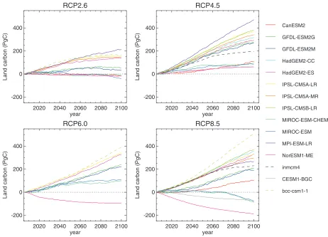
(11) 4404. JOURNAL OF CLIMATE. VOLUME 26. FIG. 3. As in Fig. 2a, but from 2005, shown separately for each RCP scenario. Individual models are denoted in separate colors for comparison across scenarios. Dashed lines represent output from ES-GCMs without represenFigure Predicted of total land carbon by the multiple CMIP-5 models for all tested tation of1.1: land-use change changes (INM-CM4.0 and BCC-CSM1.1).. scenarios using 2005 as the reference (figure taken from Jones et al. (2013)). Colors indicate different models, and dashed lines correspond to models without land use change. According to from 2151 to 127 PgC from vegetation and from 231 to the interscenario spread. Figure 3 shows each scenario Jones et soil al. (2013), all scenarios but RCP-4.5 include a net loss of naturalrelative vegetation due to to better land show 1120 PgC from (including litter) carbon. separately, anomalized to 2005 Arorause. et al. (2011) estimate the observation-based the future changes in each scenario clearly. For RCPs 2.6 cumulative historical (1850–2005) land carbon uptake, and 8.5, which both include increasing areas of land use which ismodels difficultsuggested to observethat directly, as 211turn 6 47 PgC in their scenario, models project decreases land could into a carbon source afterfour drier and warmer conditionsin future (i.e., a source to the atmosphere) as the residual of the land carbon storage, although most models project an observed change the in Amazon atmospheric carbon burden andJones increase. RCPs 4.5 and 6.0, whose scenarios include collapsed forest (Cox et al., 2004; et al., For 2009), recent evaluations constraining cumulative fossil-fuel emissions based on the CMIP5 decreasing areas of land use, all models agree on future with observed variability and sensitive increases analysis ofinseparate forcing (temperature, dataset the andresults observation-based estimates of cumulative land carbon storage, althoughrainwith large ocean carbon uptake based on Sabine and Feely (2007) spread, with RCP4.5 showing the largest values of land fall, and CO2 ) indicated that such collapse is unlikely due to the positive effect of CO2 fertilization up to 1999 and extended to 2005 using values from carbon accumulation. Denman(Cox et al.et(2007). The Huntingford wide range inethistorical landNevertheless, At present, is notgeneration easy to quantify thesystem impact of land al., 2013; al., 2013). theitnew of Earth carbon uptake among models is the result of intermodel use on the terrestrial carbon cycle within a single model Jones al. the (2013) compared the 2predictions the new generation of Earthsimulations. system models fertilizationfrom uncertainty in et both strength of the CO without carrying out multiple These simueffect (Arora et al. 2013) as well as differences in the lations are being carried out by some groups as part of also see Fig. 1.1), and large range of potential changes still exist, although simulations manner (CMIP-5, they implement land-use change. This estimate the LUCID–CMIP5 activity but are not part of the of net land carbon change very close to the multimodel CMIP5 in protocol (Brovkin et al. 2013). with the least landisuse change (RCP-4.5) generallystandard shows increase land carbon stores. mean of 219 PgC, and the range encompasses 9 out of b. Changes in ocean carbon uptake and storage 13 models (Fig. 2), although this cannot be partitioned Whether expressed as annual fluxes (Fig. 4, top) or into changes in vegetation and soil carbon separately. Only one model falls outside twice this observa- 2 cumulative changes in inventory (Fig. 4, bottom), ocean tional uncertainty: GFDL-ESM2M simulates a loss of carbon storage shows a consistent picture for each RCP across most ES-GCMs. Oceanic uptake is driven pri124 PgC..

(12) While these predictions suggest that CO2 fertilization effect could significantly enhance forest resilience by increasing water use efficiency, and thus mitigate impacts from warmer and drier climates, there is still great uncertainty on the actual contribution of the atmopsheric CO2 enrichment to biomass accumulation. The impact of CO2 on photosynthesis at the leaf level has been extensively studied and has been relatively well characterized for decades (c.f. Farquhar et al., 1980; Collatz et al., 1991; Leuning, 1995; von Caemmerer, 2000; Lambers et al., 2008) and such knowledge has been used as the basis for most dynamic global vegetation models (DGVMs) (e.g. Sellers et al., 1996; Foley et al., 1996; Oleson et al., 2010; Clark et al., 2011), but the scaling from leaf to ecosystem level, and from the typical time scale of photosynthesis controls to long term dynamics at tropical forests is far from trivial (Körner, 2009, and references therein). In addition, changes in CO2 and climate are unlikely to be the same across all species: for instance, several studies have suggested that lianas are becoming more abundant in tropical forests and their high leaf area relative to total mass ay be a reason for their faster growth (Schnitzer and Bongers, 2011); if this increase has been caused by the ongoing CO2 increase, then the net effect of CO2 enhancement can be significantly reduced. Recently, Clark et al. (2013) assessed the long term measurements of above-ground net primary productivity (ANPP) at La Selva, a tropical rainforest site in Costa Rica, and did not find any evidence of CO2 fertilization effect over the past decade, and were unable to identify an increase in ANPP due to increasing CO2 ; instead, wood production was more (negatively) correlated with nighttime temperature and vapour pressure deficit. Likewise, Zhao and Running (2010) used the MODIS net primary productivity algorithm to estimate the NPP variability and trends over the past decade, and their estimates suggested that global NPP may have marginally decreased, and that the decrease was mostly due to droughts in the Southern Hemisphere, in particular in 2005, which coincided with a major drought in the Southwestern Amazon (Marengo et al., 2008). The Amazon is the largest contiguous tropical rainforest, with the area within the Amazon Basin extending over 5.8 million km2 (Keller et al., 2004b) and storing nearly 100 Pg of carbon (Baccini et al., 2012, see Fig. 1.2 for estimated distribution of biomass across the region from. 3.

(13) GYF. 5°N 0°N. S67 S83. M34 5°S. NAT. 10°S. BAN. RJA. 15°S. PNZ. BSB. 20°S PDG 70°W. 60°W. 50°W. 40°W. Above-ground biomass [kgC m-2]. 0. 5. 10. 15. Figure 1.2: Above-ground biomass distribution across tropical South America, using the dataset from Baccini et al. (2012). Grey lines are political boundaries and the white line corresponds to Amazonia (Amazon Basin plus the Guiana Shield). The position of several sites that will be used throughout this dissertation are shown for reference. dataset), and it has been the focus of a large scientific efforts under the Large-Scale Biosphere Experiment in Amazonia (LBA Keller et al., 2004b; Davidson et al., 2012). The LBA project aggregated a wide range of multi-disciplinary studies involving researchers from numerous institutions, areas of knowledge, and countries, towards better understanding how the Amazon region would respond to future changes in climate and land use. In spite of the significant progress in knowledge brought by LBA, many questions remain open to date. One such question is exactly on how resilient to droughts the Amazonian forests will be should the frequency of droughts increase, and whether the forest is approaching a tipping point in which large areas of the forest could be lost and replaced by a lower biomass, more open canopy ecosystem akin to savannahs (Nobre and 4.

(14) Borma, 2009; Marengo et al., 2011a). The Amazon has experienced at least four major droughts over the past 25 years, most notably 1991-1992 and 1997-1998 in the North and East, and 20042005 and 2010 in the Southwestern part, (Davidson et al., 2012)), and some areas of the Amazon, particularly the Southern part, may be experiencing a drying trend (Fu et al., 2013). Controlled field experiments simulating reduction of 50% of rainfall at two locations in the Amazon showed significant increase in mortality after 3 years of the experiment, with large trees being particularly susceptible (Nepstad et al., 2007; da Costa et al., 2010). In addition, Phillips et al. (2009) found significant decrease in net biomass accumulation over large areas of the Amazon following the 2005 drought, and later Phillips et al. (2010) using pantropical data also found higher mortality amongst larger trees following droughts. While observed mortality cannot be directly attributed to droughts and confounding effects such as windthrow due to squall lines (Negrón-Juárez et al., 2010), results from remote sensing suggest that significant changes in the forest structure occurred after the drought and these changes persisted for several years (Saatchi et al., 2013). Several numerical modelling studies have been carried out testing the possibility of savannization in the Amazon, and generally found that large areas of the Amazon may be vulnerable to become either savannahs or dry forests, particularly in Southern Amazonia, and when the CO2 fertilization effect is not included (e.g. Lapola et al., 2009; Senna et al., 2009; Rammig et al., 2010). While such studies provide important insights on vulnerable areas and contain sophisticated and realistic representation of ecosystem processes, their representation of the vegetation is often simplistic and biome-based as opposed to individual-based. The relevance of individualbased becomes evident from studies showing the response of plant community to climate extremes. For example, mortality in plant communities following a climate extreme is strongly dependent on abiotic and biotic variability in the micro-environment, and rates are also strongly dependent on different tolerances between species (Allen et al., 2010, and references therein); moreover, as mentioned before, both the controlled experiments and observations from tropical forests have indication mortality rates amongst larger trees, and also varied across different genera (Nepstad et al., 2007; da Costa et al., 2010). Different responses within the plant community are not restricted. 5.

(15) to the Amazon: for example, Carnicer et al. (2011) found that while Mediterranean species responded to increasing drought and warming with increased defoliation and mortality, the response varied significantly amongst different species. Furthermore, plant community significantly alters the local environment, and results from such modifications may further affect the dynamics of the plant community as well as the establishment and maintenance of populations at longer term. For instance, recently De Frenne et al. (2013) used plant presence data from forest inventories in Europe and North America, and found that increase in presence of warm adapted understory species over the past decades was lower at denser forests. Finally, disturbances are also important drivers of the plant community dynamics, and vegetation structure and floristic composition is often significantly different depending on the disturbance history: for example, Chambers et al. (2009) compared the forest structure and floristic composition of two areas near Manaus (M34 Fig. 1.2), one undisturbed region and another that had been affected by a large blowdown event, and found significantly lower average wood density, basal area, and above-ground biomass in the disturbed area, with significantly higher abundance of typical pioneer genera such as Pouroma, Cecropia, adn Vismia at the area affected by blowdowns. Likewise, Xaud et al. (2013) found that areas affected by multiple fires in transitional forests in Roraima had significantly lower stature and basal area, and higher abundance of Cecropia. Given the relevance of distribution of individuals and micro-environments within the ecosystems, many authors have advocated that the next generation of predictive ecosystem models must be based on individuals as opposed to average properties of the biomes (e.g. Moorcroft, 2006; Purves and Pacala, 2008; van der Molen et al., 2011; Evans, 2012). Amongst individual based models, the Ecosystem Demography Model (Moorcroft et al., 2001) solves the dynamics of the ecosystem by accounting for individuals of different sizes and life strategy groups, and different patches characterized by the type of disturbance that last occurred and the time since last disturbance. More importantly, the basic equations that describe the ecosystem do not require solving every individual and every single patch; instead, it solves the probability distribution function of patch ages for each disturbance type, and for any given patch, it solves the demographic density of. 6.

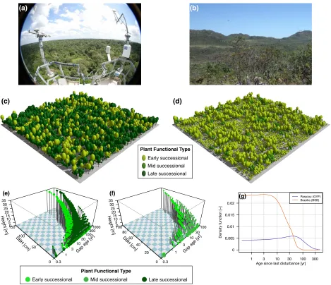
(16) each plant functional group by size. This model has previously applied to a wide range of applications and biomes (e.g. Moorcroft et al., 2001; Albani et al., 2006; Desai et al., 2007; Medvigy et al., 2009; Ise and Moorcroft, 2010; Fisher et al., 2010; Antonarakis et al., 2011; Kim et al., 2012). Recently, Powell et al. (2013) compared the ability of a suite of dynamic vegetation models to represent the results from the throughfall exclusion experiments in the Amazon, and found that the Ecosystem Demography model had a better prediction of the timing of biomass loss, presumably due to a more realistic representation of the processes and interactions and competition between individuals. How the model represents the structure of the population and landscape at a variety of biomes is illustrated in Fig. 1.3, for typical tropical rainforest and a woody savannah sites. It can be observed that in ED-2.2 biomes are also emerging properties that come with the distribution of size and age: for example, Paracou (GYF) has a low disturbance regime, which allows a high density of stems to develop (Fig. 1.3c) whereas in Brasília (BSB) a high disturbance regime (Fig. 1.3d) generated a low density of trees of generally lower stature. Moreover, the population community is structurally different between the sites (Fig. 1.3e,f), with absence of tall trees at recently disturbed sites and high abundance of early successional trees, as opposed to old patches, where mid or late successional trees become more common, and in general the population of small trees is greater amongst small trees living in old cohorts. In addition, the differences in the plant community emerge from different probability density functions of patches (Fig. 1.3g), being several times higher for recently disturbed patches, and an absence of very old patches (older than 100 yr) in Brasília.. 1.2. Thesis overview. Because of the relevance of the Amazon forest in the global context of changes in climate, carbon stocks, and biodiversity, it is fundamental to understand how resilient the ecosystem is to changes in climate that may push it outside the optimal conditions. In this context, the main goal of this dis-. 7.

(17) (a). (b). (c). (d). Plant Functional Type Early successional Height − Paracou, GUF − Meteorological forcing : WMO−based Height − Brasilia, DF − Meteorological forcing : WMO−based Mid successional Structure : Size structure − Target # of patches = 30 Structure : Size structure − Target # of patches = 30 PFTs used : 2 Grasses + 3 Trees PFTs used : 2 successional Grasses + 3 Trees Late Phenology scheme : Drought − ED−2.1 Phenology scheme : Drought − ED−2.1 Fire model : Water−deficit based Fire model : Water−deficit based Time : May / 1982 Time : May / 1982. ●. ●. ●. ●. ●. ●. ●. ●. 60. G. ●. ●. ●. 20. ● ● 0. 0.3. Plant Functional Type. Early successional Early tropical Late tropical Mid successional. ● ● ●● ● ●● ● ● ● ● ● ● ● 3 ● ●. ● ●. 40. 1. 10. Density function [−]. ●. 1. Plant functional type. ● ●● ● ● ● ●●● ● ● ● ● ● ●●● ● ● ●● ● ● ● ● ● ● ● ● ● ● ● ● ● ● ● ● ●● ●● ● ●● ● ● 100 ● ● ● ● ● ● ● ● ● ● ●● ●● ● ● ● ● ● ● ● ● ●● ● ● ● ● ● ● ● ●● ● ● 30 ●● ● ● ● ●●● ● ● ● ● ●● ●● ● ● ● ● ● ● ● ● ●. ]. [y r]. ag. e. 0. 0.02. ●. 80. Paracou (GYF) Brasilia (BSB). ●. ● ●. ap. ● ●. ●. ●● ● ●●● ● ● ●● ● ●● ● ●● ●● ● ● ●● ● ● ● ●● ● ● ● ● ● ●●● ●●● ●● ● ● ● ● ●●● ●● ●●● ● ● ● ●● ● ● ●● ●. ] m. ● ● ● ●. ●. (g). ● ● ● ● ●● ●. [c. ] m. [c. ●. ●. ●● ● ●●. BH D. BH. D. ●. ]. ]. 50. ●●●. 35 30 25 20 15 10 5 0 100. ht [m. ht [m. ● ● ●. 100. ● ● ●●. Heig. Heig. 35 30 25 20 15 10 5 0 150. Age structure. ●. (f). [y r. ●● ●. 0.015 0.01 0.005. e. ● ● ● ●. ● ● ● ● ● ● ●● ● ● ● ● ● ●● ●● ●● ● ● ●● ● ● ●● ● ●● ● ● ● ● ● ● ● ● ● ● ●● ● ●● ● ●● ● ● ● ● ● ● ● ● ● ●● ●● ● ● ● ● ●● ●● ● ● ● ● ● ● ● ● ● ● ● ● ●●●● ● ● ● ● ●● ● ● ● ●●●● ● ●● ● ● ●● ● ● ●● ● ● ● ●● ● ● ● ● ● ●●● ● ●●●●●●●● ● ●● ● ● ● ● ● ● ● ● ● ● ● ● ● ● ● ● ● ● ● ●●●● ● ● ● ● ● ● ● ● ● ● ● ● ● ● ● ●●●●● ● ● ● ● ● ● ● ● ● ● ●●● ● ● ● ●● ●● ● ● ●●● ● ● ● ● ● ● ●● ● ● ● ● ● ●●●●● ●● ● ● ● ● ●●●● ● ● ● ● ● ● ● ● 1000 ● ● ● ●●● ● ● ● ● ● ● ●● ● ●● ● ● ● ● ● ●● ●● ● ● ● ● ● ● ●● ● ● ● 300 ● ● ●●● ● ● ● ● ● ● ●● ● ● ●●● ● ● ● ● ● ● ● ● ● ● ● ● ● ● ● 100 ● ● ● ● ● ● ● ● ● ●● ●●● ● ● ● ● ● ● ● ● ● ● ● ● ● ● 30 ● ● ● ● ●● ●●● ● ● ● ●●● ● ● ● ● ● ● ●● ● ● ● ● ●● ●● 10 ● ● ● ● ● ● ● 3 ● ● ● ● ●. ag. ●. ap. ●●. G. ●. (e). 0.3. 0 1. 3 10 30 100 Age since last disturbance [yr]. 300. Plant functional type. Late successional Early tropical Mid tropical. Figure 1.3: Overview on how the size and age structure represents different biomes, (a) Paracou (GYF), a tropical rainforest site in French Guiana, and (b) Brasília (BSB), a woody savannah site at the Cerrado region in Brazil. Model representation of (c) GYF and (d) BSB at near equilibrium stage (Sec. 3.4.1). Distribution of cohorts within (e) GYF and (f) BSB(), by size (diameter at the breast height and DBH and height), age since last disturbance (gap age) and functional group (colors). Dot size is proportional to the logarithm of population of individuals within each patch. (g) Distribution of ages since last disturbance at both locations. Photograph credits: (a) http:// www.ecofog.gf/spip.php?article365, and (b) Enzo Todesco. See Fig. 1.2 for location of both sites in South America. sertation is to estimate how much shift in the rainfall regime at different areas of the Amazon forest could stand before they experienced major significant losses. In addition, I aimed at identifying how the plant community structure and composition could change should the Amazon responded 8.

(18) to drier climates. To answer this question, I used the Ecosystem Demography Model, which has the unique way of representing the structure of the biome in terms of individuals, and their ability to access and compete for resources that are needed for plants to maintain their living tissues, grow and reproduce, and represent their death in case they fail to access such resources or are affected by some other disturbance. Model development and improvement was a major part of this dissertation, and this effort was largely done in collaboration with Ryan G. Knox. The first version of the Ecosystem Demography model (Moorcroft et al., 2001) had a very simplistic representation of biophysical processes, which limited its use for understanding the impact of changes that strongly depend on processes that occur in high frequency. A major improvement in the biophysics had been carried out by Medvigy (2006), and the work presented here is largely built on top of his development; nevertheless, many issues had to be addressed before I could effectively use the model for this work. First, the model had been previously tested only for forest sites, and several original assumptions and phenomenological formulations would cause instabilities over non-forested regions. This eventually lead us to develop a much improved biophysical model, which is now derived from formal derivations from thermodynamic laws, and the system of prognostic equations is based on enthalpy and internal energy as opposed to temperature. In Chap. 2, I present the development of the version 2.2 of the Ecosystem Demography Model (ED-2.2), with particular emphasis on the new thermodynamic closure, and all modules necessary to close the enthalpy, water, and carbon dioxide cycles. In addition, I present detailed description of all modules that directly contribute to the aforementioned cycles, including hydrology and energy exchange between soil layers; the updated two-stream model for resolving the distribution of irradiance throughout the canopy; the surface layer model, which simulates the eddy covariance fluxes leaving the canopy, and the exchange of heat and water between the different surfaces and the canopy air space; the updated leaf physiology model, which controls photosynthetic activity and transpiration loss; and the autotrophic and heterotrophic respiration model. While this chapter is heavily mathematical, it constitutes an important reference for future model developments. The work in this chapter is in preparation for submission to a journal with focus on model development. 9.

(19) (e.g. Geoscientific Model Development). In Chap. 3, I present an extensive model evaluation of the current model against multiple data sets to determine the main strengths and areas where further development of the model are needed. First I evaluate the model with imposed plant community structure from forest censuses, and drive the model using site-level measurements at several locations in tropical South America, mostly but not exclusively at the Amazon forest, and compare results with eddy covariance towers, additional auxiliary measurements, and values reported from publications, in order to determine the main source of uncertainties, and identify potentially confounding effects. In addition, I compare equilibrium vegetation simulations starting from near bare ground conditions for the same locations plus additional sites located either at the transition or outside the Amazon, in order to evaluate whether the model can reproduce the variability between sites and across the region. Finally I evaluate the differences in the model dynamics towards equilibrium by using the ED-2.2 compared with simplified versions in which size, age, or functional diversity are averaged. This extensive evaluation will be also prepared as a companion publication for Chap. 2 on the same journal. In Chap. 4, I present the results on the estimates of the vulnerability of Amazonian forests to a drier climate. Here I focus on two sites with the most data on biophysical and long term dynamics available, that also have a significant seasonality and interannual variability of rainfall — Paracou (GYF) and Santarém km 67 (S67), and develop multiple rainfall regime scenarios that are based on long-term rainfall observations at both locations. I start by presenting the comparison between the observed and modelled dynamics, and explore the predicted response to increasingly drier scenarios, first looking into the effects on the community as a whole, where I observed that while Paracou showed very little response to increasingly drier conditions due to the excessive average rainfall, in Santarém km 67 the forest could start losing significant biomass at relatively modest shifts in climate, with the actual magnitude being dependent on soil conditions and plant drought adaptations. In addition, I analyse the structural changes in plant community for the simulations that showed the most response, and found that while all plants could experience higher mortality,. 10.

(20) evergreen, early successional, and larger trees had most losses and least recovery, whereas in some cases losses of the most vulnerable trees was compensated by the increase of population of trees with lower demand. Finally, I also identified the return period of extreme of sufficiently long droughts, defined as a consecutive period of 12 months with water deficit, could be used to predict areas most vulnerable to droughts, and calculated the return period from multiple rainfall data sets to estimate which regions would be the most vulnerable to drying climate. While the extreme South and Eastern Amazonia were also predicted to be as vulnerable as previous works, a large band crossing the northern and central areas of the Amazon, along with drier areas in Bolivia and Peru, could also be less resilient particularly if the average rainfall decreased. The main findings in this chapter is being prepared for submission to Ecological Applications. In Chap. 5 I present a summary of the main findings, along with suggestions for future work that could improve our understanding of the response and resilience of tropical forests to future changes in climate and land use. Finally, a significant amount of work also done in collaboration with Ryan Knox was to couple the Brazilian Regional Atmospheric Modelling System (BRAMS, K. Longo et al., 2013) to the Ecosystem Demography model. This coupling also required extensive model development of the atmospheric component, from ensuring that the thermodynamic laws between the two models were consistent to improvements on cumulus parameterizations, planetary boundary layer turbulence, and the feedbacks of parameterized clouds on radiation profile. The coupled model system is currently being used to evaluate the feedbacks between the ecosystem and the atmosphere under predicted changes in land use in South America, in particular how future change in land use from realistic scenarios (e.g. SimAmazonia Soares-Filho et al., 2006; Merry et al., 2009) could affect the distribution of heat and rainfall within the Amazon, and how this could further affect the dynamics of the remaining forests. This is an ongoing project, thus it has not been included in this dissertation. Nevertheless, the resulting coupled model has been also actively used for research led by other researchers, and the first results of this collaborative development have been submitted for publication (Knox et al., 2013a,b).. 11.

(21) Chapter 2 Enthalpy, water, and carbon-dioxide cycles in the Ecosystem Demography Model, version 2.2 The developments and improvements to the biophysical and biogeochemical parameterizations of ED-2.2 were done in collaboration with Ryan Knox, David Medvigy, and Naomi Levine.. 2.1. Introduction. Modelling the interactions between vegetation and the atmosphere has evolved considerably over the past decades (Levis, 2010). In one of the first studies analysing the interaction between biosphere and atmosphere, Charney et al. (1975) obtained a significant increase in rainfall over the Sahara by only lowering the Saharan albedo to values typical of plant-covered landscape; a few years later, Deardorff (1978) demonstrated that predictions of near surface temperature for a wheat field in England could be substantially improved by including a bulky parameterization of vegetation that became the first generation of “big leaf” models, later extended and modified to provide global surface boundary conditions (e.g., NCAR/BATS, Dickinson et al., 1986). The next genera-. 12.

(22) tions of biosphere models increased in complexity by including more mechanistic representation of radiation transfer, roughness and transpiration (e.g. SiB, Sellers et al., 1986), and some representation of photosynthesis and respiration for prescribed biomes (e.g. TEM, LSM, and SiB2, Raich et al., 1991; Bonan, 1995; Sellers et al., 1996, respectively). Meanwhile, several biogeographic models were being developed to predict the global distribution of potential equilibrium biomes based on mean climate conditions (e.g. BIOME and MAPSS, Prentice et al., 1992; Neilson, 1995, respectively), although processes such as establishment, competition, and mortality were still incipient and were largely independent of the biophysical processes. In 1996, Haxeltine and Prentice and Foley et al. presented a new approach in which competition and dominance of different plant functional types (PFTs) was directly related to the productivity, linking processes occurring at high temporal frequency such as net primary productivity to long-term dynamics. By also including climate variability, Foley et al. introduced the concept of dynamic global vegetation model (DGVM), by which changes in climate could also shift the ecosystem out of equilibrium. Later developments of DGVMs, such as LPJ (Sitch et al., 2003), CLM-DGVM (Levis et al., 2004) and TRIFFID/JULES (Hughes et al., 2004; Clark et al., 2011) among others, also included mechanisms such as disturbance through fires and multiple types of mortality due to the various constraints on biome. Although DGVMs are capable of reproducing the main patterns of the current biome distribution (e.g. Sitch et al., 2003; Blyth et al., 2011), there is still a significant uncertainty on how the ecosystems may respond to climate change, in part because of the uncertainties on the impact in regional climate, but also because of the uncertainty of how the ecosystems may respond to any given change, as discussed by Sitch et al. (2008). In particular, transitions between closed-canopy forests and treeless biomes are much sharper in these models when compared with observations (Good et al., 2011). One reason for such result is that the classic definition of PFT is blurred between individual and biome characteristics: Purves and Pacala (2008) mentioned that PFTs are defined from a combination of biogeographic range, and some very simple morphological aspects; however, they lack variation in height (or rooting depth) and function in the ecosystem. As a result,. 13.

(23) plant communities are often represented as a single vegetation type, preventing a proper representation of complex interactions between individuals that form this biome (Moorcroft, 2006; Evans, 2012). Both the traits and developmental stage of a plant are fundamental explaining its ability to compete for resources. For example, in forest ecosystems, tree size determines how much water and light an individual can access, and its physiological and life history traits determine how much resources are needed, and how efficiently the individual can obtain such resources compared to other individuals that are also accessing the same resources. Experimental studies indicate that biodiversity can enhance the ecosystem function, especially if they are carried out for longer periods (e.g., Tilman and Downing, 1994; Naeem and Li, 1997; Cardinale et al., 2007), while some studies carried out on dry lands suggest that biodiversity could contribute to enhanced ecosystem functionality in highly stressed environments (Jucker and Coomes, 2012). An alternative approach to most big-leaf based DGVMs are the individual based vegetation models, also know as gap models (c.f. Bugmann, 2001). These models simulate the birth, growth, and death of individual plants, hence incorporating the heterogeneity of the plant community. Since birth and death are stochastic processes, multiple realisations are required to determine the longterm, large-scale dynamics of these models, which limits its applicability over large regions or global scale. The Ecosystem Demography Model (ED), developed by Moorcroft et al. (2001), specifically addresses the need to incorporate heterogeneity in the plant community while remaining deterministic. The equations that describe the plant community are derived from the individual properties, but properly scaled in order to obtain the dynamics of the distribution of demographic density as a function of the individual size and PFT, and the age since the last disturbance, later extended to by Albani et al. (2006) to account for the type of disturbance; this approach was originally named the size- and age-structured model (Moorcroft et al., 2001), and along this text will be referred to as the size-, strategy-, and age-structured model (SSAS), Strategy has been included in the name to stress that unlike most DGVMs, PFTs in ED are defined not only based on biogeographic range, but, as pointed out by van der Molen et al. (2011), they also represent plant strategical properties, or dif-. 14.

(24) ferent functional groups within the same community, which is often considered more descriptive of ecosystem functioning than strict taxonomic classes (Hooper et al., 2002; Reiss et al., 2009). These functional groups represent a suite of physiological, morphological, and life history traits, thereby mechanistically representing the different ways plants utilise resources, although this also requires knowing how such traits vary in the plant community of interest (Fisher et al., 2010). The original formulation of the ED model had a very simple representation of the biogeophysical processes that drive the energy, water, and carbon dioxide (CO2 ) cycles. Since the inception of version 2, there has been an ongoing effort towards a more comprehensive and mechanistic representation of the biogeophysical and biogeochemical cycles (Medvigy, 2006; Medvigy et al., 2009; Knox, 2012). In this chapter I describe the state of the improved biogeophysical and biogeochemical module in the most recent version of the model (ED-2.2), with a special focus on processes that occur in sub-daily scale. While one will notice that many parameterizations and sub-models in ED-2.2 are based on other DVGMs, one fundamental difference, is that in ED-2.2 all biogeophysical properties are those of a horizontally and vertically heterogeneous plant community and define the resource availability and micro-environment of the different individuals within the plant canopy. In Sec. 2.2, I present a general overview of the model, including the multiple hierarchical levels associated with the SSAS approach, the different time scales associated with the model, and the input data required to drive the model. In Sec. 2.3, I present an overview of the fundamental prognostic and diagnostic equations used to determine the enthalpy, water and carbon dioxide cycles. In Sec. 2.4, I present the main sub-models used to determine the enthalpy, water, and CO2 fluxes.. 15.

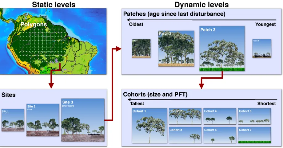
(25) Figure 2.1: Schematic of the multiple hierarchical levels in ED-2.2. Red arrows represent the nesting, showing how each parent level is split into the child groups. The definition of polygons and sites (static levels) and patches and cohorts (dynamic levels) is given in the main text.. 2.2 2.2.1. Structure of the ED-2.2 model Hierarchical levels. The solution of the plant community dynamics in ED is determined through hierarchical structures within the domain of interest and time span, as shown in the schematic in Fig. 2.1. The domain of interest is geographically divided into polygons (y): within any polygon, we assume all that time-dependent abiotic conditions such as meteorological conditions above the plant community are uniform, therefore, a polygon can be thought as a site of interest near an eddy flux tower, or the lower boundary condition for one grid column in an atmospheric model. The polygon may be subdivided into S sites; each site with fractional area As shares the same time-independent abiotic conditions such as soil texture. Both polygons and sites are defined at the beginning of the simulation and are fixed in time, and no geographic information is assumed for sites and further. 16.

(26) sub-divisions. In addition, let a[ s]1 be the age since the last disturbance of any patch of plant community within the site; i 2 {1, 2, . . . , I} be the index of the disturbance types that can generate a new patch; and a ⌘ a(a,t) be the age- and time-dependent matrix of probability distribution of age since last disturbance, where each element ai,s,y corresponds to one disturbance type i within a site of area As that satisfies. S. I. Â. i=1. Z. Â As = 1,. (2.1a). ai,s,y (a,t) da = 1.. (2.1b). s=1 •. 0. From Eqn. (2.1b), the probability can be also thought as the patch relative area within a site. Finally, let N ⌘ N(c, a,t) be the array where each element nm,i,s,y corresponds to the distribution of cohorts of same size c living in a patch of age a at time t, for each PFT m, and disturbance type i within site s of polygon y; and c = Cl ;Cr ;Cs ;Cd ;Ct [ kgC plant 1 ] is the vector that determines the size of any individual plant, and whose components are the biomass of leaves, fine roots, sapwood, structural tissues, and storage (starch and sugars), respectively. Following Moorcroft et al. (2001), Albani et al. (2006), and Medvigy and Moorcroft (2012), the fundamental partial differential equations that describe the dynamics of demographic density and probability distribution within each site in the SSAS model are defined as (dependencies omitted for clarity):. ∂ nm,i,s,y ∂ nm,i,s,y = —c · (˙gm · nm,i,s,y ) µ˙ m · nm,i,s,y , | {z }| {z } ∂t ∂ a | {z } | {z }. Change in demographic density. ∂ ai,s,y ∂ ai,s,y = ∂t } ∂a } | {z | {z | Change in Ageing. age structure. 1 Throughout. Growth. Ageing of plant community. of plant community. Mortality. I. l˙ i,i0 ai,s,y , Â 0. i =1. {z. Disturbance. }. this text, units of variables will be shown between square brackets.. 17. (2.2a). (2.2b).

(27) where µ˙ m [ s 1 ] is the mortality rate for each PFT; g˙ m [ kgC plant. 1 s 1]. is the growth rate for each. size component, and —c · is the divergent operator for the size vector; l˙ i,i0 [ s 1 ] is the disturbance rate from a patch of type i to a patch of type i0 . The boundary conditions for Eqn. (2.2) are:. nm,i,s,y (c0m , a,t) =. 1 g˙ 0m · 1 S. ( ZZZ I. ÂÂ. +. s=1 i=1. nm,i,s,y (c, 0,t) =. I. |. Â. i0 =1. ai,s,y (0,t) =. |. Z. •. c0. |. "Z. 0. dm ) r˙m nm,i ai dc {z }. (1. Local recruitment. • ZZZ • c0. 0. {z. s˙ m,i0 nm,i0 ,s,y ai0 ,s,y da , {z. Plant community following disturbance. I. Â 0. i =1. |. Z. •. 0. l˙ i0 ,i ai0 ,s,y da {z. (2.3a). dm r˙m nm,i,s,y ai,s,y dc da. Recruitment from random dispersal. •. #),. ,. }. }. (2.3b). (2.3c). }. Probability of recently disturbed patch. where c0m is the size of the smallest individual; g˙ 0m is the growth rate for individuals with size c0m ; 1 is the unity vector for size; r˙m [ s 1 ] is the recruitment rate; dm is the fraction of recruits that are randomly dispersed instead of locally recruited, which depends on the PFT; and s˙ m,i ⌘ s˙ m,i (c) is the survivorship probability for a PFT m following a disturbance of type i. The model initial conditions are discussed in the next section. In addition, let CB ⌘ CB (e) be the individual carbon balance. This property plays a direct role on controlling the plant community dynamics, which is represented by the functional form of mortality (µ˙ m ⌘ µ˙ m (c,CB (e))), growth (˙gm ⌘ g˙ m (c,CB (e))), and recruitment rates (˙rm ⌘ r˙m (c,CB (e))). Carbon balance is a function of the environment perceived by the individual, here represented by the vector e ⌘ e(m, c, s, y,t, ni ) where each component represents a different environmental variable. The perceived environment ultimately determines the resource availability for the individual, therefore it depends on the individual characteristics (m, c), abiotic factors (s, y,t), and biotic factors due to the plant community where the individual lives (represented by ni , the population vector. 18.

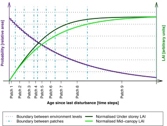
(28) within any patch). Finally, let E = E(s, y,t, ni ) be the vector of environmental conditions associated with the plant community as a whole; this vector is also a function of abiotic factors (s, y,t) and biotic factors associated with the local community (ni ), and ultimately controls the disturbance rates (l˙ i,i0 = l˙ i,i0 (E)). Because the microenvironment and plant community structure vary within the same large-scale conditions, in ED-2.2 we must solve the biogeophysical and biogeochemical cycles for each patch separately. Because Eqn. (2.2) cannot be solved analytically, the distribution of cohorts and patches is approximated by discrete classes. In principle I new patches could be created every time step taken to solve Eqn. (2.2b) and M cohorts could be created within each patch for every Eqn. (2.2a) time step, whereas older patches and older cohorts would lose area through disturbance and population through mortality. Since the number of patches and cohorts would rapidly become too large for viable simulations, it is necessary to aggregate them. Because the SSAS approach accounts for heterogeneities in the plant community environment, we aggregate patches and cohorts based on the similarity of the environmental conditions; in ED-2.2, the default method to aggregate patches of the same disturbance history is by comparing the cumulative leaf area index at multiple height levels, using the methodology illustrated in Fig. 2.2. For simplicity in this example I assume only one type of disturbance (e.g. natural disturbance), and the environment to be defined by the cumulative leaf area index (SLAI) at two height levels (in this example referred to as mid-canopy and understorey). Each environment characteristic is sub-divided into environmental levels (six levels in this example). Patches are grouped together only if their age classes are contiguous and the environmental level for each environment property. In Fig. 2.2, the widest boundary between patches is shown as vertical dot-dashed lines, and there are as many lines as times that either mid-canopy or understorey SLAI changes the environmental level. The only exception for age contiguity is when a patch is empty (i.e. no size class amongst all PFTs contain any vegetation), in which case they are all merged into a single patch. Importantly, patches are not evenly distributed in area or age, only environmental conditions. Likewise, cohorts of the same PFT that have similar DBH and leaf phenological conditions. 19.

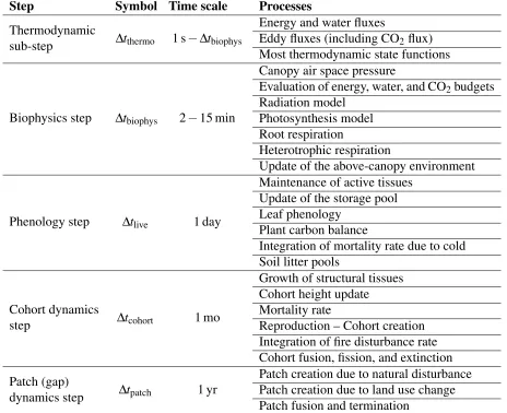
(29) Patch 9. Patch 8. Patch 7. Patch 6. Patch 5. Patch 4. Patch 3. Patch 2. Patch 1. LAI [arbitrary units]. Probability [relative area]. Age since last disturbance [time steps]. Boundary between environment levels Boundary between patches. Normalised Under storey LAI Normalised Mid−canopy LAI. Figure 2.2: Schematic of the grouping of patches for one particular land use type using environmental conditions to group different age classes. Green curves correspond to the SLAI of each height level, here shown as the relative value to the maximum SLAI of each height level, so the environmental boundaries of both classes overlap; horizontal dotted lines are the boundaries between environmental levels, and vertical dot-dashed lines are the edges between two patches. Purple line corresponds to the probability of each age class, but notice that this value is not used to define patches. may be merged. While the user may define the ideal number of patches and cohorts per patch, the actual number may be higher or lower depending on the similarities. Since ED-2.2 represents a multitude of processes that inherently have different time scales, the model also integrates different processes using a variety of nested time steps that are appropriate for each process; Tab. 2.1 contains the list with the group of processes solved by each time step. It must be noted that the biogeophysical and biogeochemical processes are dynamic: these processes are solved using a fourth-order Runge-Kutta integration scheme, which is dynamically adjusted according to error estimates.. 20.

(30) Table 2.1: Time step associated with processes resolved by ED-2.2. The thermodynamic sub-step is dynamic and it depends on the error evaluation of the integrator, but it cannot be longer than the biophysics step, which is defined by the user. Other steps are fixed as of ED-2.2. Step. Symbol Time scale. Thermodynamic sub-step. Dtthermo. 1s. Dtbiophys. Biophysics step. Dtbiophys. 2. 15 min. Phenology step. Dtlive. 1 day. Cohort dynamics step. Dtcohort. 1 mo. Patch (gap) dynamics step. Dtpatch. 1 yr. 2.2.2. Processes Energy and water fluxes Eddy fluxes (including CO2 flux) Most thermodynamic state functions Canopy air space pressure Evaluation of energy, water, and CO2 budgets Radiation model Photosynthesis model Root respiration Heterotrophic respiration Update of the above-canopy environment Maintenance of active tissues Update of the storage pool Leaf phenology Plant carbon balance Integration of mortality rate due to cold Soil litter pools Growth of structural tissues Cohort height update Mortality rate Reproduction – Cohort creation Integration of fire disturbance rate Cohort fusion, fission, and extinction Patch creation due to natural disturbance Patch creation due to land use change Patch fusion and termination. Model requirements. ED-2.2 source code is mostly written in Fortran 90, with a few file management routines written in C, with output files in HDF-5 format, and the option of running regional-level simulations in parallel mode, hence requiring HDF-5 and MPI libraries. The code uses dynamic allocation of variables and extensive use of pointers to efficiently reduce the amount of data transferred between routines. Polygon-, site-, patch-, and cohort-dependent variables are always written as long vectors that contain information from all polygons, sites, patches, and cohorts in the simulation and mapped using. 21.

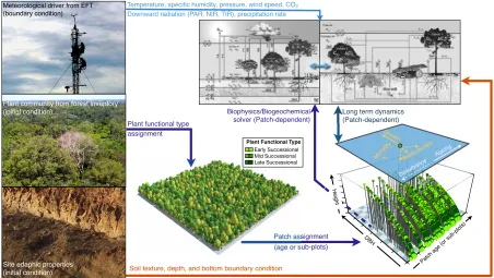
(31) Temperature, specific humidity, pressure, wind speed, CO2 Downward radiation (PAR, NIR, TIR), precipitation rate. Biophysics/Biogeochemical solver (Patch-dependent). Long term dynamics (Patch-dependent) Gr. ow. ta l M or. g. ein. Ag. e nc. b●a ●●tur● ● ● ●● ● ● ●●● ● ● ● ●● Dis●●●●●●●● ●●● ● ● ●● ● ● ●●● ●● ●● ● ● ● ● ●● ●● ● ● ●● ● ● ● ● ●● ●● ● ●● ●●● ● ● ● ● ● ● ● ● ●● ●●●● ● ● ● ● ● ● ● ●● ●●●●● ●●● ● ● ● ● ●● ● ● ● ● ● ● ● ● ●● ● ● ● ● ● ● ● ● ● ● ● ● ● ●● ● ● ● ● ● ● ● ● ● ● ● ●● ● ● ● ●● ● ●● ● ● ● ● ● ● ● ●●● ● ●●●●● ● ●● ● ●● ● ● ● ● ● ● ● ●● ● ● ● ●● ● ● ● ● ● ● ● ● ● ● ●● ● ● ● ● ● ● ● ● ●●● ● ● ●●●●●● ●● ● ● ● ● ● ●● ● ● ● ● ●● ● ● ● ● ● ● ● ● ● ● ● ● ●● ● ● ● ● ● ●● ●● ● ● ● ● ● ● ● ●● ● ● ● ● ●● ● ● ● ● ●●● ● ● ● ●● ● ● ● ● ● ● ● ● ● ● ● ● ●●● ●● ● ● ● ● ● ● ● ● ● ● ● ● ● ● ● ● ● ● ● ● ● ● ● ● ● ●● ● ●● ● ●● ●● ● ● ●● ● ● ● ● ● ● ● ● ● ●● ● ● ● ● ●●●●●● ●● ● ● ● ● ● ● ● ● ●● ● ● ● ● ● ● ● ● ● ● ● ● ● ● ● ● ● ● ● ● ● ● ● ● ● ● ● ● ● ● ●● ● ● ● ● ● ● ● ● ● ● ● ● ● ● ● ●● ● ● ● ● ●●●●● ● ● ● ● ● ● ● ● ●● ● ● ● ● ● ● ● ● ●● ● ● ● ● ● ● ● ● ● ● ● ● ● ● ● ● ● ● ● ● ● ● ● ● ● ● ● ● ● ● ● ● ● ● ● ● ● ● ● ● ● ● ● ● ● ● ●● ● ● ● ●● ● ● ● ● ● ● ● ●● ● ● ● ● ● ● ●●● ● ● ● ● ● ● ● ● ● ● ● ●● ●● ●● 2 ● ● ● ● ● ● ● ● ● ● ● ● ● ● ● ● ● ● ● ● ● ● ● ● ● ● ● ● ● ● ● ● ● ● ● ● ● ● ● ● ●● ● ● ● ● ● ● ● ● ● ●● ● ● ● ● ● ● ● ● ● ●●●● ●● ● ● ● ●● ● ● ● ● ● ● ● ● ● ● ● ● ● ● ● ● ● ● ● ● ● ● ● ● ● ● ● ● ● ● ● ● ● ● ● ● ● ● ● ● 1.8 ● ● ● ● ● ● ● ● ● ●● ● ● ● 100 ● ● ● ●● ● ●● ● ●● ● ●●●● ● ●●● ● ● ● ● ● ● ● ● ● ● ● ● ● ● ● ● ● ●● ● ● ● ● ● ●● ● ● ● ● ● ● ● ● ● ● ● ● ● ● ● ● ● ● ● ●● ● ● ● ● ● ● ●● ● ● ●● 1.6ots) ● ● ● ● ● ● ● ● ● ● ● ● ● ● ● ● ● ● ● ●● ● ● ● ●● ● ● ● 80 ● ● ●● ● ● ● ● ● ● ● ● ● ● ● ● ● ● ● ● ● ● ● ●● ● ● ● ● ●● ● ● ● ● ●● ●● ● ● ● ● ● pl ● ● ● ● ● ● ● ● ● ● ● ●●●●●●● ●● ● ● ● ● ●● ● ● ● ● ● ● ● ● ● ● ● ● ● ● ● ● b● ● ● ●● ● ● ● ● ● ● 60 ● D ● ●●●●●● ● ● ●● ●. ● ●. ●●. ]. BH. D. [c. BH. ] m. ● ● ● ● ● ● ● ● ●● ● ● ● ● ● ● ●● ● ● ● ● ● ● ● ● ● ● ● ● ●● ● 1.4u ● ● ● ● ● ● ● ● ● ● ●● ● ● ● ● ● ●● ● ● ● ● ● ● ● ● rs ● ● ● ● ● ● ● ● ● ● ● ● 1.3 ● ● ● ● ●● ● ●● (o ● ● ● ● ● ● ● ●● ● ● e ● ● ● ● ● ● ● g ●● ● ●● a ● ● ●. ●. 40. ● ●. ●. ●. 20. Soil texture, depth, and bottom boundary condition. n. [y r]. ht [m. (age or sub-plots). R●e. e. t. Heig. Heigh. Patch assignment. ctio. du. pro. ●●. 30 25 20 15 10 5 0120. Site edaphic properties (initial condition). th. ity. Plant Functional Type Early Successional Mid Successional Late Successional. ag. Plant functional type assignment. ap. Plant community from forest inventory (initial condition). ● ● ● ●● ●. ● ● ● ●. ●. ●. 0. G. Meteorological driver from EFT (boundary condition). c 1.1 at. h. P. 1. Figure 2.3: Schematic of the integration between forest inventory data, meteorological conditions, and the different modules in ED-2.2. Further description on biophysical and biogeochemical solvers is described in Sec. 2.3, and long-term dynamics description is available at Moorcroft et al. (2001); Medvigy et al. (2009). auxiliary vectors with size and count information. This approach reduces the amount of memory required and output file size, which is fundamental for long-term simulations. In addition, to ensure readability and consistency throughout the code, and allow efficient future developments, any procedure that is carried out by multiple modules is always written into functions or subroutines. In Fig. 2.3, I present an schematic of which initial and boundary conditions are necessary for running ED-2.2, and where these conditions are used. Input data falls into three main categories: demographic (initial condition), edaphic (fixed boundary condition), and meteorological (initial condition and time-dependent boundary condition). Five types of initial demographic conditions are possible in ED-2.2. To initialize a plant community from tree inventory, one must ideally have a full list of all individuals with size greater than c0 , identified to the species level, along with the coordinates or some sort of geographic information such as quadrants within the plot. If quadrants are not provided, the user may split the plot into 22.

(32) quadrants that should roughly represent the crown area of the largest trees (Moorcroft et al., 2001, e.g., 15 m ⇥ 15 m in a tropical forest); the age since last disturbance and the type of disturbance may be included if they are known, otherwise they are assumed to be old age and natural disturbance. Alternatively, initial conditions can be derived from airborne measurements, following the methodology described by Antonarakis et al. (2011). In addition, a prescribed near bare ground condition may be used: in this case a small population of cohorts nm,1 (c0 , 0, 0) = 0.1 plant m. 2. for. all PFTs is assigned to natural disturbance type, with the entire polygon being at age a = 0 and natural disturbance. For theoretical applications, it is also possible to run the model assuming no vegetation (true bare ground). Finally, plant community from previous simulations can be used to provide the initial conditions. Edaphic conditions include the predominant soil texture class or the sand, silt, and clay fraction (App. B), and the type of bottom soil boundary condition (bedrock, reduced drainage, or free drainage). Soils in ED-2.2 are generally assumed inorganic; although there is an option to assign peat, the hydraulic parameters must be manually adjusted for the site. Meteorological conditions are typical measurements of eddy flux towers and include temperature, specific humidity, CO2 mixing ratio, and pressure of the air above canopy, precipitation rate, incoming solar (shortwave) radiation and incoming thermal (longwave). Although ED-2.2 can read different variables with different time resolutions, it is highly recommended to use at least hourly resolution, or at the very least four values a day, and any gap filling on time series must be done prior to the simulation. In case of solar radiation, ideally photosynthetically active radiation (PAR) and near infrared (NIR), both split into direct and diffuse radiation, may be provided; otherwise, the total incoming shortwave radiation is split amongst these components using the Weiss and Norman (1985) model.. 23.

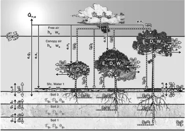
(33) 2.3. Overview of enthalpy, water, and carbon dioxide cycles. Here I present the fundamental equations that describe the biogeophysical and biogeochemical cycles. Since the environmental conditions are function of the local plant community, and resources are shared by the individuals, these cycles must be described at the patch level, and the aggregated response of the plant community can be aggregated to the polygon level once the cycles are resolved for each patch. One important assumption in ED-2.2 is that patches do not exchange enthalpy, water, and carbon dioxide with other patches, thus patches are treated as independent systems. From this point I will only refer to the patch- and cohort-levels, and indices associated with patches, sites and polygons will be omitted for clarity.. 2.3.1. Definition of the thermodynamic state. Consider that each patch is a thermodynamic envelope comprised of multiple thermodynamic systems: the soil layers, temporary surface water or snow, cohorts2 , and the canopy air space. Although patches do not exchange heat and mass with other patches, they are allowed to exchange heat and mass with the air aloft and lose water and associated internal energy through surface and sub-surface runoff. We also assume that each thermodynamic system within the patch instantaneously reaches thermal equilibrium, and that intensive variables such as pressure and temperature are uniform within each thermodynamic system. The fundamental equations that describe the system thermodynamics are the first law of thermodynamics in terms of enthalpy H [ J m 2 ], and mass continuity for incompressible fluids for total water mass W [ kgW m 2 ]:. dH = dt |{z}. Change in enthalpy 2 In. Q˙ |{z}. Net heat flux. +. H˙ |{z}. Net enthalpy flux due to mass flux. dp V | {zdt}. ,. (2.4a). Pressure correction. this section, I assume that only the above-ground part of the cohort is an independent thermodynamic system; roots are assumed to be in thermal equilibrium with the soil layers, and having negligible heat capacity compared to the soil layers.. 24.

(34) dW = dt |{z}. W˙ |{z}. (2.4b). Net mass flux. Change in water mass. where V is the volume of the thermodynamic system and p is the ambient pressure, and enthalpy and internal energy . The merit of solving the changes in enthalpy over internal energy (E) is that pressure is always included in atmospheric measurements. Nonetheless, the only thermodynamic system where this distinction matters is the canopy air space: work associated with thermal expansion of solids and liquids is several orders of magnitude smaller than heat (c.f. Dufour and van Mieghem, 1975), and changes in pressure contribute significantly less to enthalpy because the specific volume is small. Hence, for all systems except the canopy air space, changes in enthalpy are roughly equivalent to changes in internal energy, and for these systems I use internal energy and enthalpy interchangeably. Variations in internal energy and enthalpy are more important than their actual values. Therefore, enthalpy is defined as the difference between the current state and an arbitrary but predetermined and fixed reference state where we assume enthalpy to be zero. First, let Y [ kgY m 2 ] be the mass of the material and hy be the specific enthalpy of any material y [ J kgY 1 ]; because enthalpy is an extensive thermodynamic variable, the total enthalpy is the sum of enthalpies (H = Ây Yy hy ). For any material other than water (d), hd is defined as zero when the material temperature is 0 K; for water, the zero level is also at 0 K, with the additional condition that water is completely frozen. The specific enthalpy for all materials other than water (hd ), ice (hi ), liquid water (h` ) or vapor (hv ) are defined as:. hd (T ) =. qd T |{z}. (2.5a). ,. Heating material. hi (T ) =. qi T , |{z}. (2.5b). Heating ice. h` (T ) = qi Ti` + li` (Ti` ) + q` (T Ti` ), |{z} | {z } | {z } Heating ice. Melting ice. Heating liquid. 25. (2.5c).

(35) hv (T ) = qi Ti` + li` (Ti` ) + q` (T`v Ti` ) + l`v (Ti` ) + q pv (T T`v ), |{z} | {z } | {z } | {z } | {z } Heating ice. Melting ice. Heating liquid. Vaporization. (2.5d). Heating vapor. where qi and q` are the specific heats for ice and liquid water; q pv is the specific heat at constant pressure for water vapor; Ti` and T`v are the temperatures where ice melted and liquid water vaporised; and li` and l`v are the latent heat of melting and vaporization, respectively. In case ice sublimates, Eqn. (2.5d) is still valid, since liv (T ) = l`v (T ) + li` (T ) for any temperature T . By definition (e.g. Dufour and van Mieghem, 1975), the latent heat associated with phase change is the difference in enthalpy between the two phases at the temperature in which the phase change happens, therefore, we can determine the dependency of latent heat on temperature:. ∂ l`v ∂T ∂ li` ∂T. ! !. = p. = p. ∂ hv ∂T ∂ h` ∂T. !. !. p. p. ! ∂ h` = q pv q` ∂T p ! ∂ hi = q` qi ∂T. (2.6a) (2.6b). p. If we further assume that the transition between ice and liquid phases can only occur at the water def. def. triple point (T3 ), and that the latent heat of fusion li`3 = li` (T3 ) and vaporization l`v3 = l`v (T3 ) are known, we can combine Eqn. (2.5) to obtain a generic state function for h:. h=. H D W [i qi T + ` q` (T = qd T + D +W |D +W {z } |D +W {z } d. Tsc` = T3. Tscv = T3. Tsc` ) + v q pv (T. Tscv )] ,. (2.7a). w. qi T3 + li`3 , q` qi T3 + li`3 + l`v3 , q pv. (2.7b) (2.7c). where d and w are the specific mass of other materials and water, respectively, and i, `, and v are fraction of ice, liquid water, and vapor, respectively. Importantly, Eqn. (2.7a) does not contain any information about the temperature at which the phase changes had occurred, which is necessary since enthalpy must be a state function (path-independent). Hereafter, we will refer to the enthalpy as internal energy for all pools other than the canopy air space, since they are assumed equivalent, 26.

No results found