This is a repository copy of
Ram pressure stripping of the hot gaseous haloes of galaxies
using the k - ε sub-grid turbulence model
.
White Rose Research Online URL for this paper:
http://eprints.whiterose.ac.uk/82594/
Version: Published Version
Article:
Close, JL, Pittard, JM, Hartquist, TW et al. (1 more author) (2013) Ram pressure stripping
of the hot gaseous haloes of galaxies using the k - ε sub-grid turbulence model. Monthly
Notices of the Royal Astronomical Society, 436 (4). 3021 - 3030. ISSN 0035-8711
https://doi.org/10.1093/mnras/stt1788
[email protected]
https://eprints.whiterose.ac.uk/
Reuse
Unless indicated otherwise, fulltext items are protected by copyright with all rights reserved. The copyright
exception in section 29 of the Copyright, Designs and Patents Act 1988 allows the making of a single copy
solely for the purpose of non-commercial research or private study within the limits of fair dealing. The
publisher or other rights-holder may allow further reproduction and re-use of this version - refer to the White
Rose Research Online record for this item. Where records identify the publisher as the copyright holder,
users can verify any specific terms of use on the publisher’s website.
Takedown
If you consider content in White Rose Research Online to be in breach of UK law, please notify us by
MNRAS436,3021–3030 (2013) doi:10.1093/mnras/stt1788
Advance Access publication 2013 October 11
Ram pressure stripping of the hot gaseous haloes of galaxies using the
k
−
ǫ
sub-grid turbulence model
J. L. Close,
1‹J. M. Pittard,
1T. W. Hartquist
1and S. A. E. G. Falle
2 1School of Physics and Astronomy, University of Leeds, Leeds LS2 9JT, UK2Department of Applied Mathematics, University of Leeds, Leeds LS2 9JT, UK
Accepted 2013 September 19. Received 2013 September 5; in original form 2013 April 18
A B S T R A C T
We perform three-dimensional hydrodynamic simulations of the ram pressure stripping of the hot extended gaseous halo of a massive galaxy using thek−ǫsub-grid turbulence model at
Mach numbers 0.9, 1.1 and 1.9. Thek−ǫmodel is used to simulate high Reynolds number
flows by increasing the transport coefficients in regions of high turbulence. We find that the initial, instantaneous stripping is the same whether or not thek−ǫmodel is implemented and is in agreement with the results of other studies. However the use of thek−ǫmodel leads to five times less gas remaining after stripping by a supersonic flow has proceeded for 10 Gyr, which is more consistent with what simple analytic calculations indicate. Hence the continual Kelvin–Helmholtz stripping plays a significant role in the ram pressure stripping of the haloes of massive galaxies. To properly account for this, simulations of galaxy clusters will require the use of sub-grid turbulence models.
Key words: hydrodynamics – methods: numerical – galaxies: clusters: general – galaxies: evolution – galaxies: haloes.
1 I N T R O D U C T I O N
The properties of galaxies that exist in clusters differ from those of galaxies that exist in the field. This is the so-called morphology– density relation (Dressler 1980). A higher local galaxy density is correlated with a larger fraction of late-type (elliptical, E/S0) galax-ies (Goto et al. 2003). It is also associated with a number of other galactic properties, including a decreased rate of star formation (G´omez et al. 2003) and a higher fraction of red galaxies (Balogh et al. 2004). Also, dwarf elliptical galaxies are more strongly clus-tered than dwarf irregulars (Binggeli, Tammann & Sandage 1987; Binggeli, Tarenghi & Sandage 1990). These observational results strongly suggest that a cluster environment shapes the evolution of the galaxies within it.
One possible way to explain the morphology–density relation is ram pressure stripping. This was first explored analytically for a disc shaped gas distribution by Gunn & Gott (1972). As a galaxy orbits within a cluster it moves though the inter-cluster medium (ICM) which exerts a ram pressure on the gas in the galaxy. Ram pressure stripping can be separated into two distinct processes: instantaneous stripping and Kelvin–Helmholtz stripping. The instantaneous strip-ping occurs when the ram pressure is higher than the gravitational force per area on a column of gas and occurs on short time-scales (less than 1 Gyr in most cases). Kelvin–Helmholtz stripping is due to the shear force created as the ICM flows past the edge of the galaxy. This induces the Kelvin–Helmholtz instability (KHI) and
⋆E-mail: [email protected]
allows material to be continually stripped from the galaxy and oc-curs on longer time-scales. Ram pressure stripping has led to tails in a number of galaxies in the Virgo cluster (Crowl et al. 2005; Abramson et al. 2011).
A number of studies have been done to try to quantify different aspects of this effect. In general, the effect of ram pressure stripping is simulated in two ways. First one can perform a ‘wind tunnel’ test. Here the galaxy is placed in a constant wind to simulate the effect of the galaxy moving though the ICM. This allows parameters, like the relative speed of the ICM and galaxy, to be precisely controlled. The other method is to allow the galaxy to orbit within a cluster potential. This gives a more realistic representation of ram pressure stripping and includes tidal effects (which may or may not be desirable).
Many studies have been performed to investigate the effect of ram pressure stripping on spiral galaxies. Abadi, Moore & Bower (1999) used a smoothed particle hydrodynamics (SPH) code to simulate a three-dimensional spiral galaxy undergoing ram pressure stripping. Although their results match those of the analytic approach of Gunn & Gott, it cannot account fully for the observations. Roediger & Br¨uggen (2006) looked specifically at the role of the inclination angle of the disc and its effect on the morphology of the galaxy, using a grid-based code. They found that the mass loss of the galaxy
is relatively insensitive to the inclination angle for angles<≃60◦.
They also noted that the tail is not necessarily pointing in the same direction as the motion of the galaxy. J´achym et al. (2009) also looked at the role of inclination angle but used a SPH code. They find much the same dependence on inclination angle as Roediger & Br¨uggen (2006) although they saw no Kelvin–Helmholtz stripping.
C
2013 The Authors
Published by Oxford University Press on behalf of the Royal Astronomical Society
at University of Leeds on January 22, 2015
http://mnras.oxfordjournals.org/
Tonnesen & Bryan (2009) allowed the gas in the disc of the spiral galaxy to radiatively cool before being hit by the wind to allow areas of low and high density to develop. They found that gas is stripped more rapidly in the case with cooling as areas of lower density allow gas to also be stripped from the inner regions of the galaxy.
A number of studies have instead been focused on dwarf galaxies. Mori & Burkert (2000) looked at the stripping of the extended hot gas component using a two-dimensional grid-based code. They found that the gas is totally stripped in a typical galactic cluster. Mayer et al. (2002) simulated a dwarf galaxy orbiting the Milky Way
with anN-body code to probe the tidal effects on the dwarf galaxy
and found a significant mass loss over a period of 7 Gyr. Mayer
et al. (2006) used a combination of SPH andN-body simulations
to study the combined effects of ram pressure and tidal stripping on dwarf galaxies. They pointed out that tidal effects can alter the morphology of the dwarf galaxy and change the effectiveness of ram pressure stripping. In general, this increases effectiveness but tidally induced bar formation can funnel gas towards the centre of the galaxy, making it harder to strip.
In addition to these works a few papers contain results of work specifically on the effect of ram pressure stripping on the hot ex-tended component of the gas. McCarthy et al. (2008) simulated a massive galaxy with a hot halo of gas undergoing ram pressure stripping. They performed both wind tunnel tests and simulations allowing the galaxy to orbit within a cluster to include tidal effects. They extended the analytic model of Gunn & Gott (1972) to the case of a spherical gas distribution and found that their formula fits simulations well when the galaxy represents less than 10 per cent of the cluster mass. They suggested that at this point tidal effects and gravitational shock heating become important, which their model does not take into account. Bekki (2009) included both a hot halo and a disc in their model and suggested that the presence of the disc can suppress ram pressure stripping. Shin & Ruszkowski (2013) used a grid-based code to look at the effects of turbulence within the ISM. They found that this increases mass loss and allows the ICM to penetrate further into a galaxy.
2 T U R B U L E N C E M O D E L
The majority of studies on ram pressure stripping have been per-formed with SPH codes. While these can model the effect of in-stantaneous stripping, they are known to have difficulty resolving KHIs correctly (Agertz et al. 2007). Typically studies done with SPH codes show little to no Kelvin–Helmholtz stripping, whereas it is seen in studies done with grid-based codes. However, grid-based codes are also currently unable to reproduce the turbulence actu-ally involved in ram pressure stripping. The turbulent behaviour of
a flow depends on its Reynolds number, Re= ur/ν, whereuis
the velocity of the flow,r is the typical length scale of the flow
andνis the kinematic viscosity. In this work we takeras the
ra-dius of the galaxy after instantaneous stripping. For a fully ionized,
non-magnetic gas of densityρ and temperatureT, the kinematic
viscosity
ν=2.21×10⁻¹⁵T 5/2A1/2
Z4ρlng cm 2
s−1, (1)
whereAandZare the atomic weight and charge of the positive ions
and lnis the coulomb logarithm (Spitzer 1956).
We can estimate the Reynolds number of the ICM using the
above equations. Takingv=580 km s−1as the flow speed past the
galaxy, r= 79 kpc as the characteristic size of the galaxy after
instantaneous stripping,ρ= ×1.7×10⁻²⁸g cm−3andT
=107K
as the ICM density and temperature,A≈1.0,Z≈1.0 and ln≈
30, givesν≈1.35 cm2s−1andRe
≈100 for the ICM gas for pure
hydrodynamics.
However, the ICM contains a magnetic field, which is typically
of the order of 1µG (see e.g. Carilli & Taylor 2002). If the
ther-mal velocity is≈5×107cm s−1(appropriate for 107K plasma),
then the particle gyroradius≈2.5×1010cm. Since this is small
compared to the size of the largest turbulent eddies, the ions are constrained to move along the field. For the tangled fields that one would expect, this leads to a considerable reduction in the viscosity, which means that we can safely assume that we are dealing with large Reynolds number turbulence, certainly too large for direct numerical simulation.
The only tractable method to describe such flows is a statistical approach. We therefore use a sub-grid turbulent viscosity model in an attempt to calculate the properties of the turbulence and the
resulting increase in the transport coefficients. Thek−ǫmodel is
widely used and appropriate in this context. The earliest develop-ment efforts on this model were by Chou (1945). The closure coef-ficients were subsequently adjusted by Launder & Sharma (1974) to create the accepted ‘standard’ model, and its popularity has led to it featuring extensively in textbooks (e.g. Pope 2000; Davidson
2004; Wilcox 2006). It introduces two extra fluid variables:k, the
turbulent energy per unit mass andǫ, the turbulent dissipation rate
per unit mass. Turbulence is modelled through the use ofkandǫto
calculate a turbulent viscosity which increases the transport coeffi-cients in regions of high turbulence. In this paper we use the term ‘inviscid’ to refer to simulations performed without the use of the
k−ǫmodel.
The equations that determinekandǫare largely empirical, but
have been used to great success in engineering and in some astro-physical problems (Falle 1994; Pittard et al. 2009; Pittard, Hartquist & Falle 2010). For instance, we found in Pittard et al. (2009) that
k−ǫsimulations of the turbulent ablation of clouds showed much
better convergence in resolution tests than inviscid simulations,
and that the converged solution in thek−ǫmodels was in good
agreement with the highest resolution inviscid models. Of course, other possibilities and variations also exist for modelling turbulent flows. For instance, Scannapieco & Br¨uggen (2008) use a model
similar to the k − ǫ model to capture the Rayleigh–Taylor and
Richtmyer–Meshkov instabilities and buoyancy-driven turbulence in active galactic nuclei, and Schmidt & Federrath (2011) recently developed a sub-grid model for highly compressible astrophysical turbulence.
Thek−ǫmodel used has been shown to give reasonable
agree-ment with experiagree-ment for turbulent underexpanded jets with Mach
numbers in the range 1–2 and density contrasts≈2 (Fairweather &
Ranson 2006). This gives us some confidence in the present sim-ulations since both problems involve the growth of turbulent shear layers and the dimensionless parameters are not very different: the Mach numbers are similar, the density contrast in the galactic shear
layer is≈10 and the Reynolds numbers are large in both cases.
3 H Y D R O DY N A M I C S
3.1 Method of simulation
In thek−ǫmodel the equations (Pittard et al. 2009) describing
con-tinuity, momentum, energy, scalar, turbulent energy and turbulent dissipation are, respectively,
∂ρ
∂t + ∇ ·(ρu)=0, (2)
at University of Leeds on January 22, 2015
http://mnras.oxfordjournals.org/
Ram pressure stripping using the k
−
ǫ
model
3023
∂ρu
∂t + ∇ ·(ρuu)+ ∇P− ∇ ·
τ=ρg, (3)
∂E
∂t +∇ ·[(E+P)u−u·
τ]− γ
γ−1∇ ·(μT∇T)=ρu·g, (4)
∂ρC
∂t + ∇ ·(ρCu)− ∇ ·(μT∇C)=0, (5)
∂ρk
∂t + ∇ ·(ρku)− ∇ ·(μT∇k)=Pt−ρǫ, (6)
∂ρǫ
∂t + ∇ ·(ρǫu)− ∇ ·(μǫ∇ǫ)= ǫ
k(C1Pt−C2ρǫ). (7)
ρis the mass density,uis the velocity,Pis the thermal pressure
andEis the total energy density (thermal and kinetic).Crepresents
any advected scalar. In this case we use only one, to distinguish
between the galactic gas and the ICM.C1 =1.4 andC2= 1.94
are both constants. g is the gravitational field. We use a static
gravitational field to simulate the effect of dark matter, as described in Section 3.2. The effects of gas self-gravity are neglected as the gravitational field is assumed to be dominated by the dark matter.
The effect ofkandǫon the other fluid variables is characterized
by
μT=ρCμ k2
ǫ, (8)
and
μǫ= μT
1.3, (9)
whereCμ =0.09.Ptis the turbulent production term. Using the
summation convention,
Pt=μT
∂
ui
∂xj
∂
ui
∂xj +
∂uj
∂xi
−2
3∇ ·u(ρk+μT∇ ·u). (10)
τis the turbulent stress tensor and is defined as
τij =μT
∂ui
∂xj +
∂uj
∂xi
− 2
3δij(ρk+μT∇ ·u). (11)
The equations simplify to the familiar inviscid equations fork=0.
The values ofC1,C2andCμ are determined by the requirement
that a variety of experimental results are matched by model results (Dash & Wolf 1983). So they are not free parameters. The maximum turbulent length scale must also be chosen, which limits the size of the largest eddies. We choose the predicted radius of the galaxy after instantaneous stripping, 120 kpc, as the appropriate value. Tests indicate that the simulations are not very sensitive to this parameter, with the biggest differences being in the far downstream structure of the wake. Importantly the turbulent mixing layer around the galaxy is not affected by our choice of the maximum turbulent length scale, and therefore the rate of stripping within our model is robust.
The calculations were performed with the hierarchical adaptive
mesh refinement (AMR) code, MG. The code uses the Godunov
method, solving a Riemann problem at each cell interface, using piece-wise linear cell interpolation and MPI-parallelization. The equations (2)–(7) are solved using the second-order upwind scheme described in Falle (1991) for the hyperbolic terms combined with
a centred difference for the diffusive terms. A hierarchy ofNgrids
levels,G0· · ·GN−1, is used, and the mesh spacing forGnisx/2n,
wherexis the cell size for the coarsest level,G0.G0andG1cover
the entire domain, but finer grids need not do so. Refinement is on a
cell-by-cell basis and is controlled by error estimates based on the difference between solutions on different grids, i.e. the difference
between the solutions on Gn−1 and Gn determine refinement to
Gn+1. The efficiency is increased by using different time-steps on
different grids, such thatGnundergoes two steps for each step on
Gn−1. In these calculationsG0had 50 cells per side and there were
five additional levels of refinement, giving a maximum resolution of 1600 cells per side, corresponding to a minimum mesh spacing of 6 kpc.
3.2 Initial conditions
We take the galaxy to comprising a dark matter halo and a hot extended gas component. We followed McCarthy et al. (2008) for the dark matter and gas density distributions. We used an NFW distribution (Navarro, Frenk & White 1996) for the dark matter:
ρ(r)dm=
ρs
(r/rs)(1+r/rs)2
. (12)
The characteristic density of the dark matter halo is
ρs= Ms
4π r3
s
, (13)
where
Ms=
M200
ln(1+c200)−c200/1+c200
, (14)
c200=r200/rsis the concentration parameter and we takec200=4
in accordance with McCarthy et al. (2007).r200 is the radius at
which the average density is 200 times the critical density,ρcrit=
3H2
0/8π G.M200is the mass withinr200. We assumed the dark matter
causes a static gravitational field. In the absence of tidal forces we do not expect the dark matter distribution to be significantly altered; so a static field is justified. The dark matter extends to a radius of r25≈2.44r200.
The initial hot gas component was assumed to follow the dark matter distribution, such that
ρg(r)=fbρt(r), (15)
where ρb is the gas density, ρt is the total density and
fb= 0.022h−2/0.3=0.141 is the universal fraction of baryonic
matter. The gas distribution of the galaxy is truncated at r200.
The temperature and density of the ICM were set to 107K and
10−4cm−3. Hydrostatic equilibrium of the halo gas was assumed
and determines the temperature and pressure distributions. The gas
contained withinr200 was given an advected scalar so that mass
from the galaxy could be identified at later times. The total initial
mass of the hot gaseous halo is 5.64×10¹¹M
⊙. The galaxy was
allowed to evolve in isolation with and without thek−ǫmodel
implemented and is stable for many Gyr.
The initial values ofkandǫwere set to 3×10¹⁰erg g−1and to
3×10¹⁰erg g−1, respectively. As these values are several orders
of magnitude lower than those subsequently generated during the interaction, the effect of the turbulent viscosity is dominated by the real turbulence at all times. We note that a positive feature of
thek−ǫmodel is its relative insensitivity to the initial conditions
forkandǫ(see e.g. section 5.4.3 of Wilcox 2006).
The ICM was given an initial velocityU1in the positivex
direc-tion to simulate the effects of the galaxy moving though it. The lower
xboundary is set to drive the wind at the same speed throughout the
simulation. In reality a galaxy falling into a cluster will see a gradual increase in wind speed. This will cause the instantaneous stripping phase to be drawn out over a longer period of time. By the onset
at University of Leeds on January 22, 2015
http://mnras.oxfordjournals.org/
Table 1. Galaxy model parameters. Variable Value
M200 2×10¹²M⊙
c200 4
fb 0.141
[image:5.595.103.226.71.138.2]rs 79 kpc
Table 2. ICM parameters. Variable Value(s)
n0 10−4cm−3
T0 107K
Mach number 0.9, 1.1, 1.9
of continual stripping however, enough time has passed (∼2 Gyr)
that any shocks caused by the initial impact have dissipated. Three different velocities were used, corresponding to Mach numbers of
0.9, 1.1 and 1.9 (U1= 470 km s−1, 580 km s−1and 1000 km s−1,
respectively). These values are typical of those in the literature and representative of the orbital speeds of a cluster galaxy. Simulations for each different Mach number were performed with and without
thek−ǫmodel. A summery of the parameters used can be found
in Tables 1 and 2.
3.3 Parametrization of galaxy mass
In order to measure the mass of the gaseous component of the galaxy as a function of time, and hence the effectiveness of ram pressure
stripping, we track the mass in four ways.Mg,r200, the mass of gas
that was initially part of the galaxy and is within a distance ofr200
of the galactic centre.Mg,unmixedthe mass of gas that was initially in
the galaxy and that is in cells in which at least half of the gaseous
material started the simulation in the galaxy.Mg,bound,gal, the mass
of gas that was initially in the galaxy that is gravitationally bound
to the dark matter potential.Mg,bound, the total mass of gas that is
bound to the dark matter potential.
3.4 Effects of resolution
In order to investigate the effects of resolution, we ran the high-est Mach number simulation with one extra refinement level. The bound mass for these tests is shown in Fig. 1. At early times both methods give similar results, which is not surprising since the in-stantaneous stripping is unaffected by turbulence. At later time the
k−ǫmodel converges, whereas there is no evidence of convergence
in the inviscid runs. The inviscid calculations can be regarded as Implicit Large Eddy Simulations since the numerical algorithm has the required properties (Aspden et al. 2008), but such calculations are clearly not reliable unless one can achieve convergence. This we have been unable to do even though we have used higher resolution than in previous calculations such as Shin & Ruszkowski (2013).
The advantage of thek−ǫmodel is that it converges at a
res-olution that can be used in practical calculations. We also have shown results for a run with one less refinement level using the
k−ǫmodel. At this resolution the results begin to diverge from the
higher resolution runs.
Figure 1. Mg,boundas a function of time for a Mach number of 1.9. The
results for the model incorporating thek−ǫmodel are shown in green. Those for the inviscid model are in red. The solid lines are for the standard resolution used throughout the rest of this study, the dashed lines are for the runs with an extra level of refinement, which allowed twice the maximum resolution and the dotted line uses one less refinement level, halving the maximum resolution. The dash–dotted line has two extra refinement levels, increasing the maximum resolution by a factor of 4 to 1.5 7 kpc.
4 A N A LY T I C A L A P P R OX I M AT I O N S
4.1 Instantaneous stripping
Instantaneous stripping occurs when the ram pressure exceeds the gravitational force per unit area on a column of material. In McCarthy et al. (2008) an analytical prediction for the instanta-neous ram pressure stripping of a spherically symmetric galaxy was derived, which extended work done by Gunn & Gott (1972).
The condition for ram pressure stripping at a given radius,R, is
ρicmνgal2 > α
GMgal(R)ρgas(R)
R , (16)
whereαis a constant dependent on the dark matter and gas profiles.
McCarthy et al. (2008) found that for their wind tunnel testsα≈2
best fits their results. The stripping radius for each model is noted in Table 3. We also note the mass density and the sound speed of
the hot gaseous galactic halo at this radius (ρ2anda2in Table 3,
respectively).
4.2 Kelvin–Helmholtz stripping
The rate at which mass is lost due to the KHI was estimated by Nulsen (1982) to be
˙
Mkh=π r2ρicmνgal. (17)
Takingras the radius after instantaneous stripping from equation
(16) and using 1000 km s−1as the velocity of the galaxy we get a
mass-loss rate of 49 M⊙yr−1for the assumed galaxy. At this rate,
the hot halo would be completely stripped in 4.4 Gyr. We might expect this to be the rate at which mass is lost initially, but as mass is stripped the radius will decrease. One can assume that the mass– radius relation remains constant in order to calculate how the radius changes as mass is removed from the galaxy.
at University of Leeds on January 22, 2015
http://mnras.oxfordjournals.org/
[image:5.595.103.223.177.229.2]Ram pressure stripping using the k
−
ǫ
model
3025
Table 3. Parameters for the simulations.U1is the speed of the ICM relative to the galaxy.a1anda2are the sound speeds in the ICM
and in the galaxy at the stripping radius, respectively. The temperature and sound speed of the hot halo increases with radius.ρ2is the gas mass density of the galaxy at the stripping radius, andρ1is the density of the ICM.Ucis the predicted convective velocity of the gas
in the shear-layer (equation 19).δ′
0is the incompressible growth rate of the mixing layer (equation 18),πcis a compressibility parameter
(equation 20),δ′(πc)/δ′
0is the normalized growth rate (equation 21), andθ′(πc) is the opening angle (equation 22). For the Mach 1.1 and
1.9 models, the ICM first passes through a bowshock upstream of the galaxy. The second line for each of these models therefore contains values computed with the free-streaming ICM conditions replaced by the conditions of the immediate post-shock flow on the symmetry axis. We have assumed that the stripping radius is unchanged and therefore do not adjust the values ofa2andρ2.
Model U1 Stripping a1 a2 ρ2 ρ2/ρ1 Uc δ′0 πc
δ′(πc)
δ′
0
θ′(πc)
Mach No. (km s−1) radius (kpc) (km s−1) (km s−1) (g cm−3) (km s−1) (◦)
1.9 1000 120 526 320 4.6×10⁻²⁸ 5.5 298 0.57 2.55 0.19 6.2
460 733 2.5 346 0.44 1.17 0.39 9.8
1.1 580 202 526 380 1.4×10⁻²⁸ 1.65 254 0.39 1.25 0.37 8.2
504 550 1.44 232 0.37 1.08 0.42 8.9
0.9 470 236 526 425 0.9×10⁻²⁸ 1.13 228 0.35 0.90 0.49 9.8
4.3 Compressible turbulent shear layers
Turbulent shear layers are also of wide interest to the fluid-mechanics community and much study has been devoted to them. Brown & Roshko (1974) determined that the visual thickness of the shear layer spreads as
δ′ vis,0=
δ(x) x−x0 ≈
0.17U
Uc
, (18)
whereδ(x) is the thickness of the mixing layer at a downstream
distance ofx− x0from the point where the streams initially
in-teract,U=U1−U2is the velocity difference between the two
free streams andUc is the ‘convective velocity’ at which
large-scale eddies within the mixing layer are transported downstream. The constant 0.17 was empirically determined. When stream ‘2’ is stationary,
Uc= U1
1+ρ2
ρ1
1/2, (19)
where the densities of the free streams are ρ1 and ρ2 (e.g.
Papamoschou & Roshko 1988). A slightly more complicated form of equation (18) is noted in Soteriou & Ghoniem (1995).
It has long been recognized that the growth rate of compress-ible mixing layers is lower than predicted by equation (18) when the convective velocity is high. This is attributed to compressibility effects. Papamoschou & Roshko (1988) showed that experimental measurements of the growth rate normalized by its incompressible
value,δ′/δ′
0, was largely a function of the ‘convective Mach
num-ber’,Mc,1= (U1− Uc)/a1, wherea1is the sound speed of free
stream ‘1’. More recently, Slessor, Zhuang & Dimotakis (2000) argue that the convective Mach number under-represents compress-ibility effects for free streams with a significant density ratio, and shows that a better characterization is achieved through the use of an alternative compressibility parameter,
πc=maxi
√γ
i−1 ai
U , (20)
whereγiandaiare the ratio of specific heats and the sound speed
of free streami. Forπc3, the normalized growth rate
δ′(π c) δ′
0
≈
1+απc2
−1/2
. (21)
The opening angle of the mixing layer is then
θ′(πc)=2 arctan
δ′(π c) 2
. (22)
5 R E S U LT S
5.1 Wind tunnel tests
Fig. 2 shows snapshots of the mass density distribution at a number
of times for each of the runs. Thek−ǫruns agree relatively closely
with their counterparts during the instantaneous stripping phase, but become increasingly divergent at later times when the KHI is most important. The largest difference between the inviscid and
k−ǫsimulations is seen in the Mach 1.9 run. The results for runs
incorporating the k − ǫ model look smoother in general as the
density given is a local mean density.
Fig. 3 shows the distribution of turbulent energy for eachk−ǫ
run. The turbulence is initially produced at the interface between the galaxy and the ICM. There is also turbulence in the tail after instantaneous stripping, as seen in the central column of panels. This is initially generated during instantaneous stripping and is ad-vected downstream. At later times, the turbulence generated at the galaxy–ICM interface has managed to propagate into and fill the tail. Some of the turbulence in the tail also moves back towards the galaxy. The general trend of increased turbulence at higher Mach numbers is apparent. This is shown quantitatively in Fig. 4. At sonic and marginally supersonic Mach numbers the turbulent energy rises
gradually with time after an initial delay of∼2 Gyr while
instan-taneous stripping is occurring. The total turbulent energy peaks
at∼8 Gyr in the highest Mach number simulation as turbulence
begins to be advected from the grid. The typical value of the
turbu-lent diffusivity in the shearing layers isμT∼3×1028cm2s−1(as
defined by equation 8).
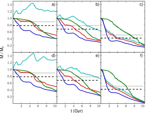
Fig. 5 shows each of the different ways we tracked the mass of the
galaxy, as described in Section 3.3. In the first∼2 Gyr gas is removed
where gravity is weak enough to be overcome by ram pressure, and Mg,bound,gal (red) and Mg,r200 decrease.Mg,unmixed (green) remains relatively constant during this period, showing that the ram pressure is not mixing the gases, but rather pushing it from the galaxy, as we might expect. This occurs on a time-scale equal to the sound crossing time (1.8 Gyr). It should be noted that in the transonic cases
much of the ICM component ofMg,boundis in front of the galaxy
and is still part of the flow. For example, in the Mach 0.9 case (shown in Fig. 6), the wind speed is equal to the escape velocity
at∼170 kpc, so gas within this radius is technically bound but is
being constantly pushed downstream due to the flow of the wind behind it. After this the galaxy enters a transitional period where little to no mass is stripped from the galaxy, particularly at lower Mach numbers. The galaxy then begins to be stripped by the KHI
at University of Leeds on January 22, 2015
http://mnras.oxfordjournals.org/
Figure 2. The mass density in thez=0 plane. The first two columns contain results for simulations at a Mach number of 0.9, the second two results for a Mach number of 1.1 and the last two results for a Mach number of 1.9. The left column in each pair shows results for the inviscid simulations, while the right column in each pair gives results for models that incorporate thek−ǫmodel.
at University of Leeds on January 22, 2015
http://mnras.oxfordjournals.org/
Ram pressure stripping using the k
−
ǫ
model
3027
[image:8.595.46.288.308.495.2]Figure 3. The distribution in thez=0 plane of turbulent energy,k, for simulations incorporating thek−ǫmodel. Rows correspond to, from the top, Mach numbers of 0.9, 1.1 and 1.9. The three times are: during instantaneous stripping, after instantaneous stripping and at the end of the simulation.
Figure 4. The total turbulent energy,Eturb, across the entire grid. The blue,
green and red lines give results for the simulations with Mach numbers of 0.9, 1.1 and 1.9, respectively.
until the end of simulation and the mass associated with the galaxy decreases.
The general shape of the curves is the same in all cases (with
the exception ofMg,bound, as noted above). The lengths of the
in-stantaneous stripping and transitional periods appear independent of Mach number, with the transitional period being more pro-nounced at lower Mach numbers. In general stripping is stronger at higher Mach numbers. In all cases the galaxy loses more mass than predicted due to instantaneous stripping alone. This means that Kelvin–Helmholtz stripping is significant on the 10 Gyr
time-scales investigated. The simulations incorporating thek−ǫmodel
differ the most from the corresponding inviscid simulation at the highest Mach number (Figs 5c and 5f), particularly in the late-time Kelvin–Helmholtz stripping phase, when the turbulence is fully developed.
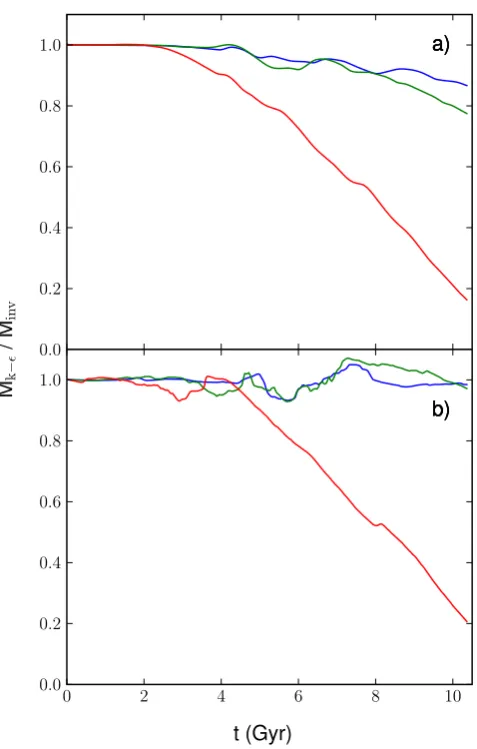
Fig. 7 shows the difference in mass stripping between the
invis-cid and thek−ǫsimulations in more detail. While there is little
difference inMg,bound,galat the transonic Mach numbers (but some
difference inMg,r200) at supersonic Mach numbers we see that there
is significantly more stripping when thek−ǫmodel is used. For
the Mach 1.9 case,Mg,r200andMg,bound,galare both only 20 per cent
of the mass in the inviscid model at late times.
Fig. 8 shows the simple analytical predictions of equation (17) for a Mach number of 1.9. The galaxy undergoes a transitional period between the instantaneous and Kelvin–Helmholtz phases, thus the time at which results should be expected to follow the analytic
prediction is unclear. For any chosen starting point after∼5 Gyr both
curves fit the simulation well initially and slowly diverge away. This suggests that although the simulation strips at a rate which is similar to the analytical prediction, the formula is an oversimplification of the time dependence of the radius.
Table 3 notes predicted values for the convective velocity,Uc, for
each simulation. However, it is not possible for us to easily com-pare our simulation results to this value because our simulations provide us with the mean local velocity instead, and this changes across the mixing layer from the undisturbed galactic halo gas to the unmixed ICM gas flowing past. In addition, Papamoschou & Bun-yajitradulya (1997) show that predictions for the convective Mach number and the convective velocity need correcting if the mixing is not ‘symmetric’. For these reasons we choose to instead focus on the opening angle of the mixing layer. The predicted opening angles for the Mach 0.9 model and the post-shock-adjusted predictions for
the Mach 1.1 and 1.9 models yieldθ′(π
c)≈10◦. This compares
with the observed angle of about 10◦–15◦estimated from Fig. 4,
and is also consistent with the results of Canto & Raga (1991) (see also the end of section 4.2 in Pittard et al. 2009). We consider this level of agreement as perfectly acceptable given that our simula-tions differ in some notable respects from the experiments we are comparing against. For instance, in our work (i) the mixing layer is not flat but instead curves around the galaxy; (ii) the ICM gas does not stream past the galaxy at a steady velocity (it is nearly station-ary close to the stagnation point of the flow upstream of the galaxy and accelerates around the galaxy); iii) the gas experiences gravi-tational forces from the galaxy. We conclude that these differences affect the opening angle of the mixing layer by less than a factor of 2.
at University of Leeds on January 22, 2015
http://mnras.oxfordjournals.org/
Figure 5. Gaseous component of the galaxy mass as a function of time for all six simulations. Results for inviscid runs are shown in a–c, and results for runs incorporating thek−ǫmodel in d–f. Columns correspond to, from the left, Mach numbers of 0.9, 1.1 and 1.9. The blue line showsMg,r200, the green line
showsMg,unmixed, the red line showsMg,bound,galand the cyan line showsMg,bound. The black dashed line is the analytical prediction from equation (16) with α=2. The black dotted line gives the result for the same equation but forα=3.
Figure 6. The distribution of gas that started the simulation as ICM and is bound to the dark matter potential, for the 0.9 Mach number model incorporating thek−ǫmodel. In the blue area the gas bound to the galaxy is mostly gas that was associated with the galaxy initially.
5.2 Comparison to previous works
McCarthy et al. (2008) investigated ram pressure stripping of a hot
galactic halo with the SPH codeGADGET-2. Our bound mass after
instantaneous stripping lies above what one would expect from
equation (16) using theα∼2 value that they determined from their
results, particularly at lower Mach numbers, which they did not investigate. The method they used for calculating bound mass is fundamentally different from ours (due to the differences in SPH and grid-based codes) and they discussed this in appendix A of their paper. They found that implementing the same bound mass calculation as we use increases the amount of mass bound after instantaneous stripping suggesting that this could be the reason for the discrepancy between our results. Our results are more consistent
withα = 3, as shown in Fig. 5. They noted that instantaneous
stripping occurs on time-scales comparable to the sound crossing time of the galaxy, which is what we found. They did not, however, see any mass loss after the instantaneous stripping period, in contrast to our results.
Bekki (2009) included a disc in the galaxy in addition to a halo
and used the SPH codeGRAPE-SPH. He only conducted two-body
tests (i.e. no wind tunnel tests), so a direct comparison with our results is not possible. However, he remarked that his results are broadly consistent with those of McCarthy et al. (2008). He also does not see any continual stripping after the initial mass loss.
Most recently, Shin & Ruszkowski (2013) used the grid-based codeFLASH3 to study ram pressure stripping of elliptical galaxies. They measured the mass of their galaxy by measuring the mass
at University of Leeds on January 22, 2015
http://mnras.oxfordjournals.org/
[image:9.595.43.284.484.628.2]Ram pressure stripping using the k
−
ǫ
model
3029
Figure 7. Ratio of the mass of the galaxy ink−ǫruns over the corre-sponding inviscid run. The top panel showsMg,r200, while the bottom panel
Mg,bound,gal. The blue, green and red lines correspond to Mach numbers of
0.9, 1.1 and 1.9, respectively.
Figure 8. Mg,boundas a function of time for a Mach number of 1.9. Shown in
green is the run incorporating thek−ǫmodel and in red is the inviscid run. The black dotted line shows the prediction from equation (17), assuming a constant radius. The black dashed line shows the same equation but allowing the radius to change over time.
within radial zones and so their results are most comparable with ourMg,r200calculations. They look specifically at subsonic galaxy speeds (Mach number of 0.25) so our results are not necessarily directly comparable but we see broadly the same pattern of quick, instantaneous stripping, followed by a plateau and then continual stripping to the end of simulation.
6 C O N C L U S I O N
We have studied the effects of ram pressure stripping on the halo of a massive galaxy using three-dimensional hydrodynamic simulations
incorporating thek−ǫsub-grid turbulence description. We have
varied the Mach number of the interaction to investigate its effect. We found that in all cases the KHI contributes significantly to the stripping of material from the galaxy. This is captured both with
and without use of thek− ǫmodel at transonic Mach numbers.
During instantaneous stripping the simulations incorporating the
k− ǫ model produces the same results as simulations in which
it is not used. However at higher Mach numbers (i.e. 1.9) Kelvin–
Helmholtz stripping is only properly captured when thek−ǫmodel
is used.
This means that the stripping of gas from hot gaseous haloes has been underestimated in previous simulations particularly those in which the galaxy Mach number is about two or more. Since it is cur-rently not feasible to accurately model fully developed turbulence in this problem, the incorporation of a sub-grid turbulence model,
such as thek−ǫmodel, is highly desirable.
R E F E R E N C E S
Abadi M. G., Moore B., Bower R. G., 1999, MNRAS, 308, 947
Abramson A., Kenney J. D. P., Crowl H. H., Chung A., van Gorkom J. H., Vollmer B., Schiminovich D., 2011, AJ, 141, 164
Agertz O. et al., 2007, MNRAS, 380, 963
Aspden A., Nikiforakis N., Dalziel S., Bell J. B., 2008, Comm. Appl. Math. Comp. Sci., 3, 103
Balogh M. L., Baldry I. K., Nichol R., Miller C., Bower R., Glazebrook K., 2004, ApJ, 615, L101
Bekki K., 2009, MNRAS, 399, 2221
Binggeli B., Tammann G. A., Sandage A., 1987, AJ, 94, 251 Binggeli B., Tarenghi M., Sandage A., 1990, A&A, 228, 42 Brown G. L., Roshko A., 1974, J. Fluid Mech., 64, 775 Canto J., Raga A. C., 1991, ApJ, 372, 646
Carilli C. L., Taylor G. B., 2002, ARA&A, 40, 319 Chou P. Y., 1945, Quart. Appl. Math., 3, 38
Crowl H. H., Kenney J. D. P., van Gorkom J. H., Vollmer B., 2005, AJ, 130, 65
Dash S. M., Wolf D. E., 1983, AIAA Paper 83-0704
Davidson P. A., 2004, Turbulence: An Introduction for Scientists and Engi-neers. Oxford Univ. Press, Oxford
Dressler A., 1980, ApJ, 236, 351
Fairweather M., Ranson K. R., 2006, Prog. Comp. Fluid Dyn., 6, 122 Falle S. A. E. G., 1991, MNRAS, 250, 581
Falle S. A. E. G., 1994, MNRAS, 269, 607 G´omez P. L. et al., 2003, ApJ, 584, 210
Goto T., Yamauchi C., Fujita Y., Okamura S., Sekiguchi M., Smail I., Bernardi M., Gomez P. L., 2003, MNRAS, 346, 601
Gunn J. E., Gott J. R., III, 1972, ApJ, 176, 1
J´achym P., K¨oppen J., Palouˇs J., Combes F., 2009, A&A, 500, 693 Launder B. E., Sharma B. I., 1974, Lett. Heat Mass Transfer, 1, 131 McCarthy I. G., Frenk C. S., Font A. S., Lacey C. G., Bower R. G., Mitchell
N. L., Balogh M. L., Theuns T., 2008, MNRAS, 383, 593 McCarthy I. G. et al., 2007, MNRAS, 376, 497
at University of Leeds on January 22, 2015
http://mnras.oxfordjournals.org/
[image:10.595.46.287.485.673.2]Mayer L., Moore B., Quinn T., Governato F., Stadel J., 2002, MNRAS, 336, 119
Mayer L., Mastropietro C., Wadsley J., Stadel J., Moore B., 2006, MNRAS, 369, 1021
Mori M., Burkert A., 2000, ApJ, 538, 559
Navarro J. F., Frenk C. S., White S. D. M., 1996, ApJ, 462, 563 Nulsen P. E. J., 1982, MNRAS, 198, 1007
Papamoschou D., Bunyajitradulya A., 1997, Phys. Fluids, 9, 756 Papamoschou D., Roshko A., 1988, J. Fluid Mech., 197, 453
Pittard J. M., Falle S. A. E. G., Hartquist T. W., Dyson J. E., 2009, MNRAS, 394, 1351
Pittard J. M., Hartquist T. W., Falle S. A. E. G., 2010, MNRAS, 405, 821 Pope S. B., 2000, Turbulent Flows. Cambridge Univ. Press, Cambridge
Roediger E., Br¨uggen M., 2006, MNRAS, 369, 567 Scannapieco E., Br¨uggen M., 2008, ApJ, 686, 927 Schmidt W., Federrath C., 2011, A&A, 528, A106 Shin M.-S., Ruszkowski M., 2013, MNRAS, 428, 804
Slessor M. D., Zhuang M., Dimotakis P. E., 2000, J. Fluid Mech., 414, 35 Soteriou M. C., Ghoniem A. F., 1995, Phys. Fluids, 7, 2036
Spitzer L., 1956, Physics of Fully Ionized Gases. Wiley, New York Tonnesen S., Bryan G. L., 2009, ApJ, 694, 789
Wilcox D. C., 2006, Turbulence Modeling for CFD, 3rd edn. DCW Indus-tries, Inc., La Canada, CA
This paper has been typeset from a TEX/LATEX file prepared by the author.
at University of Leeds on January 22, 2015
http://mnras.oxfordjournals.org/