Attitude Maneuvers
.
White Rose Research Online URL for this paper:
http://eprints.whiterose.ac.uk/81034/
Version: Accepted Version
Article:
Zhang, S., Tang, G.J., Friswell, M.I. et al. (1 more author) (2014) Multi-objective
Optimization of Zero Propellant Spacecraft Attitude Maneuvers. Journal of Optimization
Theory and Applications. 1 - 23. ISSN 0022-3239
https://doi.org/10.1007/s10957-014-0524-8
Reuse
Unless indicated otherwise, fulltext items are protected by copyright with all rights reserved. The copyright
exception in section 29 of the Copyright, Designs and Patents Act 1988 allows the making of a single copy
solely for the purpose of non-commercial research or private study within the limits of fair dealing. The
publisher or other rights-holder may allow further reproduction and re-use of this version - refer to the White
Rose Research Online record for this item. Where records identify the publisher as the copyright holder,
users can verify any specific terms of use on the publisher’s website.
Takedown
If you consider content in White Rose Research Online to be in breach of UK law, please notify us by
Multi-objective Optimization of Zero Propellant
Spacecraft Attitude Maneuvers
,S. Zhang
1 •G.J. Tang
2 •M.I Friswell
3 •D.J Wagg
4Communicated by Mauro Pontani
Abstract
The zero propellant maneuver is an advanced space station, large angle attitude maneuver technique,using only control momentum gyroscopes. Path planning is the key to success and this paper studies the associated
multi-objective optimization problem. Three types of maneuver optimal control problem are formulated: (i)
momentum-optimal, (ii) time-optimal and, (iii) energy-optimal. A sensitivity analysis approach is used to study the
Pareto optimal front and allows the tradeoffs between the performance indices to be investigated. For example, it is
proved that the minimum peak momentum decreases as the maneuver time increases, and the minimum maneuver
energy decreases if a larger momentum is available from the control momentum gyroscopes. The analysis is verified
and complemented by the numerical computations. Among the three types of zero propellant maneuver paths, the
momentum-optimal solution and the time-optimal solution generally possess the same structure, and they are
singular. The energy-optimal solution saves significant energy, while generally maintaining a smooth control profile.
AMS Classification
90C29Keywords Space station • Zero Propellant Maneuver (ZPM) • Multi-objective Optimization Problem (MOP) • Pareto optimal front • Sensitivity analysis
,
Research supported by the National Natural Science Foundation of China, grant number: 11272346.
1 College of Aerospace Science and Engineering, National University of Defense Technology, Changsha, China.
410073. Email: [email protected]
2
College of Aerospace Science and Engineering, National University of Defense Technology, Changsha, China. 410073.Corresponding author, Email: [email protected].
Ocpwuetkrv
Enkem"jgtg"vq"fqypnqcf"Ocpwuetkrv<"30Ocpwuetkrv0fqe"
Enkem"jgtg"vq"xkgy"nkpmgf"Tghgtgpegu
1 Introduction
NASA has successfully conducted two Zero Propellant Maneuver (ZPM) missions on 5 November 2006 and
3 March 2007, when the International Space Station (ISS) was rotated by 90¡ [1] and 180¡ [2], respectively. The
ZPM technique is a new concept to maneuver a space station using only Control Momentum Gyroscopes (CMGs). In
particular, the environmental torque is exploited to enable large angle maneuvers to be achieved, whilst
simultaneously maintaining the CMGs within their operational limit [3]. A ZPM is a complex attitude maneuver
guidance problem, in which maneuver path planning is the key to success. The executed trajectories of the two ZPM
missions were momentum-optimal. The momentum objective, defined in the Optimal Control Problem (OCP), gives
the maneuver path with the largest CMGs angular momentum redundancy, which brings increased robustness to the
angular momentum deviations arising from various disturbances [4]. This robustness is especially important for paths
that are planned off-line. However, the momentum-optimal path has a large rate of momentum change of the CMGs
around the initial and final times that require fast gimbal motion, which may harm the CMGs. Thus, maneuver path
types, other than momentum-optimal, should be studied, and different path types synthesized. The other types of
maneuver paths require different objectives in the ZPM OCP formulation; typical examples include the
energy-optimal and the time-energy-optimal paths. The energy-optimal energy performance index yields the maneuver path, which
minimizes the energy consumed. Since the electrical power that dives the CMGs is limited on-board, methods to
save energy have practical value. The optimal time performance index seeks the path that gives the minimum time to
fulfill the maneuver and this improved agility is required under certain situations.
The momentum-optimal solution is specific to the ZPM OCP. Although energy- or time-optimal attitude
maneuver problems have been studied for decades, the ZPM OCP version differs in a number of respects that are
now outlined. First, in a ZPM the motion of the CMGs needs to be considered and, generally, the angular momentum
of the CMGs has a final state requirement. Second, generally the ZPM is a rest-to-rest reorientation with respect to
the orbit reference frame instead of the inertial frame, and thus the rotation of the orbit frame needs to be considered.
Third, the path constraint of the ZPM is not a simple bounded control torque constraint, but is more complex since
the angular momentum and the rate of momentum change of the CMGs must be restricted within their allowable
range. Fourth, the environmental torque must be exploited to realize a ZPM, while it is neglected in the classic
optimal attitude maneuver studies. The total angular momentum of the spacecraft system, including the space station
body and the CMGs, may change greatly during a ZPM. As an angular momentum change device, the CMGs cannot
produce the angular momentum. Thus, the environmental torque is required to realize the momentum change for the
ZPM. These differences show the inapplicability of classic OCP results and highlight the necessity to study the ZPM
problem.
The three performance indices may be considered as a Multi-objective Optimization Problem (MOP). In
general, a solution, which optimizes all of the performance indices simultaneously, does not exist, and a compromise
solution has to be sought. The concept of the Pareto optimum is a widely accepted tradeoff between the objectives
[5]. Generally, the Pareto optimal set of the MOP must be determined numerically. There are two types of numerical
methods; either the MOP is transformed to a set of Single-objective Optimization Problems (SOP) to be solved, or an
evolutionary algorithm is utilized to solve the MOP directly [5]. Often large amount of computation is required to
obtain the optimal front for a complex MOP, particularly to ensure that the numerical results uncover the tradeoff
relationship with adequate accuracy. In an optimization problem, if the optimized performance index is a function of
a parameter, which may be another performance index, then the Pareto optimal front may be investigated using the
derivative, i.e. the sensitivity. For example, for a minimization MOP with two objectives, the first order sensitivity of
the optimal front curve is negative and strictly monotonic. Thus the sensitivity analysis may be used to gain insight
into the Pareto optimal front. To verify and complement the resulting conclusions, numerical computations are also
performed using GPOPS (version 5.2) [6], which employs the Radau Pseudo Spectral (PS) method [7].
The paper is organized as follows. The ZPM MOP is formulated in Section 2. Section 3 presents the
sensitivity analysis theory of the OCP objective with respect to a parameter. In Section 4, the ZPM MOP is studied,
the optimal solutions for a single objective are investigated, and the conclusions, deduced using the sensitivity
analysis method, are verified and complemented by the numerical computations.
2 Formulation of the ZPM MOP
2.1 State Equations
To derive the equations of motion, relevant reference frames are defined first. The body reference frame, b,
has its origin at the center of mass of the space station. It is fixed with the space station and its axes are aligned with
the geometric characteristic directions, which are not necessarily the principal inertia axes. The Local Vertical Local
Horizontal (LVLH) orbit reference frame,
o
, has origino
o that coincides with the center of mass of the spacestation. The
o z
o o axis is aligned with the local vertical, towards the centre of Earth, theo x
o o axis lies on theorbit plane in the transverse direction, normal to
o z
o o, and theo y
o o axis is perpendicular to the orbit plane,paper, a circular orbit is assumed for the space station, so that the orbit rotation rate, n, is constant.
The Modified Rodrigues Parameters (MRPs) are the minimal description of attitude, which avoids
singularities for a principal rotation up to
‒
360 deg [8]. They are defined as]
_
T1 2 3
: : tan
4
s
u u u
? ?e , (1)
where e is the principal rotation axis and s is the principal rotation angle. The kinematic equation which
describes the attitude of the space station with respect to the orbit is
*
+
( ) o
?T / , (2)
where T( ) is the kinematic matrix, and b( ) 0
]
0_
To?Ro /n are the space station angular velocity and
the orbit frame angular velocity, described in the body frame, respectively, b o
R is the rotation matrix from the orbit frame, o, to the body frame, b. The specific form of T( ) and b
o
R are given by Schaub et al. [8]. The dynamic equation described in the body reference frame is
*
+
1
e ( )
/
?J / / ·u J , (3)
where J is the inertia matrix of the space station, u is the control generated by the CMGs, and the “
·
” denotes the vector cross product. The environmental torques acting on the space station, e, include the earth gravity gradienttorque, the aerodynamic torque and other types of torques. Since the magnitude of the other environmental torques is
much smaller than that of the gravity gradient torque and the aerodynamic torque, they are neglected in the path
planning problem. The models for the gravity gradient torque and the aerodynamic torque are given by Bhatt [4].
The motion of the CMGs must also be considered in the maneuver, because of their limited capacity and the
boundary condition constraints. The equation of motion of the CMGs is
cmg? / · cmg
h u h , (4)
where
h
cmg is the angular momentum of the CMGs described in the body frame. In order to apply the analysistheory developed in next section, here the pseudo-control
w
is defined ascmg
:? / ·
w u h . (5)
The transformation of the control does not affect the solution of the OCP, but it guarantees the rigorousness of the
sensitivity analysis. Equations (3) and (4) are transformed to
*
+
1
e ( cmg)
/
?J / / ·w J -h , (6)
cmg?
h w. (7)
2.2 Boundary Conditions
Generally, a ZPM transfers the space station from one Torque Equilibrium Attitude (TEA) to another. For a
TEA, the attitude and corresponding angular velocity are associated, and the CMGs momentum state is prescribed
for the momentum management [4]. The general form of the initial and final boundary conditions is
0 0 0 0 cmg 0 0
( )t ? , ( )t ? , h ( )t ?h, (8)
cmg
( )tf ? f, ( )tf ? f, h ( )tf ?hf, (9)
where t0 is the initial time, and tf is the final time. In this paper, the initial time t0 is set to be zero, so that tf
represents the maneuver time. 0, 0, h0 and f, f, hf are the prescribed initial and final boundary
conditions, respectively.
2.3 Path Constraints
CMGs have limits on their angular momentum and torque. Hence, during a maneuver the CMGs must operate
within their performance range, which may be written as constraints on the angular momentum and the rate of
angular momentum change [4] as
2 2 cmg hmax
h , (10)
and
2 cmg 2
max d
dt h
h , (11)
where hmax and hmax are the momentum magnitude parameter and the rate of momentum change magnitude
parameter, respectively. Note that the path constraints involve the Euclidean norm squared to ensure they are
differentiable at zero. The first constraint is called the momentum constraint, which is a state constraint. The second
constraint is called the rate of momentum change constraint. Using the control transformation given by (5), it may
be transformed to a pure control constraint from a mixed state-control constraint.
2.4 Objectives
Three objectives are considered for the ZPM, namely the momentum objective, the time objective and the
energy objective. The momentum objective represents the peak angular momentum of the CMGs during the
maneuver, and takes the form
This objective is equivalent to a Mayer objective
i
( )
t
f , which may be induced by regardingi
as a state variable with state equation,i
?
0
. The momentum-optimal control problem seeks the solution with minimum peak momentum during the maneuver, i.e. r: m n? i i.The time objective is the maneuver time. Thus
2: f
J ?t . (13)
The maneuver time in the time-optimal control problem is denoted as v ?: mintf.
The energy consumed during the maneuver is an important measure of the control performance. In the paper
the energy is represented by the integral of the square control torque, which is related to the energy consumed. Thus,
the performance index is
0 0
T T
cmg cmg
d ( ) ( ) d
: tf tf
t t
E ?
Ð
u u t?Ð
w- ·h w- ·h t, (14)and the energy objective is
3
:
J
?
E
. (15)The energy performance in the energy-optimal control problem is denoted as e: m n? i E, which has units of N2m2s
rather than energy.
The ZPM MOP is now defined. The objectives are given by (12), (13) and (15), the state equations are
given by (2), (6) and (7), the boundary conditions are given by (8) and (9), and the path constraints are given by
(10) and (11).
3 Sensitivity Analysis
Consider a parameter in the optimization problem. Then the optimal performance index is a function of that
parameter, and the analytical form of this function is often impossible to obtain explicitly. An alternative is to study
the derivative, i.e. the sensitivity, of the function to the parameter about a baseline value. The first order sensitivity
represents the tangent slope and the second order sensitivity represents the convexity. Generally, the sign of these
two sensitivities determines the basic shape of the function, thus uncovering the influence of parameter changes on
the optimal value. If the parameter is the value of one of the performance indices, then the sensitivity gives
information on the Pareto optimal front.
Rehbock et al. [9] calculated the first order sensitivity of the optimal performance index with respect to a
static parameter, but the result is limited to the unconstrained OCP with free final states. In this section, the
sensitivity with respect to static parameters is generalized to the constrained OCP. Because the final time
t
f isoften an important parameter as well as a performance index, the sensitivity to
t
f is also presented. For thesubsequent studies, an initial assumption is that, if a solution to the OCP exits, then it is continuously differentiable
with respect to the perturbation parameter of interest [10].
Lemma 3.1 The constrained optimal control problem is given by
* +
i : m n
K ? J , (16)
subject to 0 0 ( , , ; ), ( ( ), ; ) , ( ( ), ; ) , ( , , ; ) , ( , ; ) , f f t a
t t a t t a
t a t a
?
? ?
x f x u
x 0 x 0
C x u 0 S x 0
where
0
( ( ), ; ) ( , , ; )
: f f ttf d
J ?h x t t a -
Ð
L x ut a t, x is the n dimensional state variable vector, u is the m dimensionalcontrol variable vector, a is the static parameter, and the final time
t
f may be fixed or free. In (16), x? f is the state equation, and and are the initial and final boundary conditions, respectively. C and S are pathconstraints, and represent the mixed state-control inequality constraint and the state inequality constraint
respectively. Then, the sensitivity to the static parameter is calculated as
0 0 d ( )d d f t
a f a a t a
K
H t
a ? © ! © - -h
Ð
, (17)
where H:? - © - © - ©L f S C is the augmented Hamiltonian, 0 and f are the Lagrange multiplier
parameters, is the costate vector,
v
and are the Karush-Kuhn-Tucker (KKT) multiplier variables, and the“
©
” denotes the vector dot product. The subscript a denotes the partial derivative with respect to a, for examplea
a
• ?
• .
Lemma 3.1 may be proved by investigating the variation of the objective functional with respect to the
variation of the parameter along the optimal solution. Thus, (17) is obtained from
*
+
*
+
*
+
*, * d
min ( , , ; ) ( , , ; )
da J t a a J t a
• ?
• x u
x u x u , (18)
where
0
0 ( ( ) )d
: f ttf
J ? © +r © +h-
Ð
L- © f/x - ©S- ©C t is the augmented objective obtained through thedirect adjoining method [11], and x* and u* denote the optimal solutions corresponding to a specified parameter
a. Note that the sensitivity given by Rehbock et al. [9] is a special case of (17).
Lemma 3.2 For the constrained optimal control problem given by (16) with fixed final time
t
f,d
( )
d f tf tf f
f
K
H t
t ? © -h
-, (19)
where H:? - ©L f is the Hamiltonian.
Lemma 3.2 is proved in the same way as Lemma 3.1. Equation (19) is consistent with the first order
optimality condition when the final time is free. When the sensitivity is zero, i.e. d 0 d f
K
t ? , the optimal condition
with respect to the final time variation is obtained.
It will be shown that, by utilizing the property of the boundary conditions or KKT multiplier, the signs of the
first order sensitivities presented in the Lemmas may be determined without solving the OCP, thus presenting
qualitative results. The treatment in the presence of state inequality constraints is complex. When there are both state
inequality constraints and mixed state-control inequality constraints, the applicability of the direct adjoining method
is not fully proved. In [11], several specific cases are listed. When the mixed state-control inequality constraint is
independent of the state, reducing to a pure control inequality constraint, the applicability is proven. The reason why
the pseudo-control is defined in (5) is to guarantee the applicability of the theory developed here.
4 Study of the ZPM MOP
In this section, the optimal solutions for single objectives are investigated first. Then, the three objectives are
considered in pairs to understand the tradeoffs between the objectives. Finally, the results are synthesized to gain
insight into the potential solutions. To verify and complement the analytical results obtained, a common example
taken from [4] will be used. The maneuver is an approximate −90 deg rotation from a +XVV TEA to +YVV TEA. The orbital rotation rate is n=1.1461!10-3 rad/s, and the inertia matrix of the space station is
2 24180443 3780009 3896127
3780010 37607882 -1171169 kg m 3896127 -1171169 51562389 Ç
È Ù
? È Ù
È Ù
É Ú
J .
The constraints for the CMGs are a maximum momentum of hmax= 1.9524!10
4
Nms and a maximum rate of
change of momentum of hmax= 271.16 Nm. The aerodynamic model utilizes a mass density of the atmosphere of
2!10-11kg/m3, and the drag coefficient is 2.2. The space station body includes two parts: the center body and the solar arrays. The center body is modeled by a quasi-cylinder of length 45m and radius 2.25m. The solar arrays are
represented by two symmetrical plates of length 20m and width 4m. Described in the body frame, The vectors from
the total mass center to the pressure centers are assumed to be fixed, and given by [-0.17, -0.10, 4.50]Tm and [-0.17,
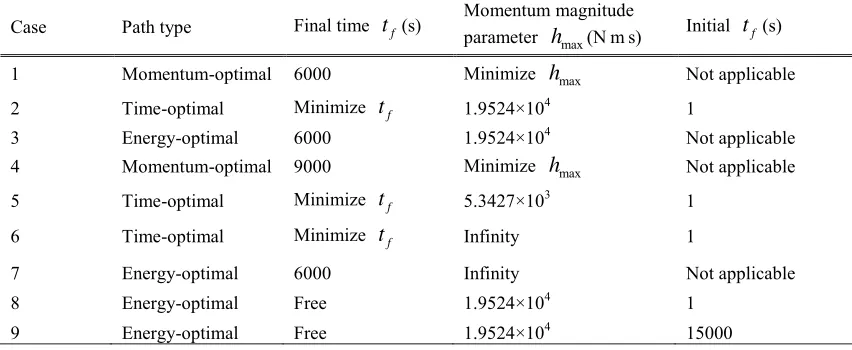
-0.10, -9.00]Tm, respectively. Table 1 gives the initial and final boundary conditions. Several typical ZPM OCPs
will be designed, and these are detailed in Table 2. Note that hmax is the optimization parameter in the ZPM
[image:10.595.83.503.224.292.2]momentum-optimal problem, and its value is intentionally changed in some numerical computations.
Table 1 The initial and final boundary conditions for the ZPM mission
Initial state Value Final state Value
0 [0.1352, -0.4144, 0.5742] T
!10-1 f [-0.3636, -0.2063, -4.1360]T!10-1
0(rad/s) [-0.2541, -1.1145, 0.0826] T
!10-3 f(rad/s) [1.1353, 0.0030, -0.1571]
T
!10-3
0
h
(Nms) [-672.4768, -237.2650, -5276.7736]Th
f(Nms) [-12.2022, -4822.5806, -183.0330]T
Table 2 The designed ZPM path planning cases
Case Path type Final time
t
f(s) Momentum magnitudeparameter
h
max(Nms) Initialt
f(s)1 Momentum-optimal 6000 Minimize
h
max Not applicable2 Time-optimal Minimize
t
f 1.9524!104 13 Energy-optimal 6000 1.9524!104 Not applicable
4 Momentum-optimal 9000 Minimize
h
max Not applicable5 Time-optimal Minimize
t
f 5.3427!103 16 Time-optimal Minimize
t
f Infinity 17 Energy-optimal 6000 Infinity Not applicable
8 Energy-optimal Free 1.9524!104 1
9 Energy-optimal Free 1.9524!104 15000
4.1 Optimal Solutions for a Single Objective
The solutions for momentum-optimal, time-optimal and energy-optimal control problems (corresponding to
ZPM cases 1 to 3 in Table 2, respectively) were computed. The related results show the characteristics of different
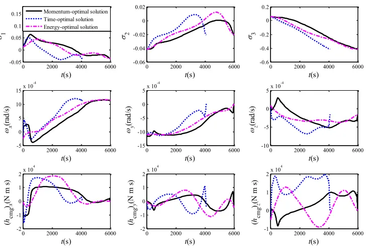
types of ZPM paths. The state solutions of the three OCPs are presented in Fig. 1. It is shown that, for the
momentum-optimal and time-optimal solutions, the angular velocity changes sharply near the initial and final time.
The profiles of the components of the CMGs momentum for the three solutions, (hcmg)x and (hcmg)y, are similar,
while the components (hcmg)z are obviously different.
[image:10.595.85.511.325.500.2]0 2000 4000 6000 -0.05 0 0.05 0.1 0.15 t(s) u1
0 2000 4000 6000 -0.06 -0.04 -0.02 0 0.02 t(s) u 2
0 2000 4000 6000 -0.6 -0.4 -0.2 0 0.2 t(s) u 3
0 2000 4000 6000 -5
0 5 10 15x 10
-4
t(s)
y(rax
d
/s
)
0 2000 4000 6000 -15
-10 -5 0 5x 10
-4 t(s) yy (ra d /s )
0 2000 4000 6000 -10
-5 0 5x 10
-4
t(s)
y(raz
d
/s
)
0 2000 4000 6000 -2
-1 0 1 2x 10
4
t(s)
(
hcm
g )x (N m s )
0 2000 4000 6000 -2
-1 0 1 2x 10
4
t(s)
(
hcm
g )y (N m s )
0 2000 4000 6000 -1
0 1 2x 10
4 t(s) ( hc m g )z (N m s ) Momentum-optimal solution Time-optimal solution Energy-optimal solution
Fig. 1 The state solutions of the three ZPM OCPs
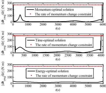
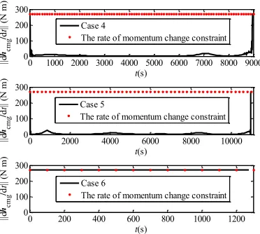
Figure 2 presents the momentum magnitude profiles and Fig. 3 presents the rate of momentum change
magnitude profiles. For the energy-optimal solution, the momentum constraint is active for about 900s, and the rate
of momentum change profile is smooth. The momentum-optimal and time-optimal solutions have the same structure.
The rate of momentum change constraint is active near the initial and final time, and the momentum constraint is
active at intermediate times. This phenomenon may be explained physically. For the time-optimal solution, the rate
of momentum change constraint is active to provide the largest control. The CMGs then maintain the maximum
momentum to yield the largest possible angular velocity. At the end of the maneuver, the angular momentum of the
CMGs must decrease quickly to reach the prescribed final boundary condition. So, the rate of momentum change
constraint is active again. For the momentum-optimal solution, the final time is fixed and the peak momentum is
maintained for as long as possible. Hence, to reduce the time for the momentum of the CMGs to change between the
boundary value and the peak value, the rate of momentum change reaches the threshold, in a similar way to the
[image:11.595.119.483.120.366.2]0 1000 2000 3000 4000 5000 6000 0 0.5 1 1.5 2 2.5
3x 10
4 !(s) || h cm g ||( N m s ) Momentum-optimal solution Time-optimal solution Energy-optimal solution The momentum constraint
Fig. 2 The CMGs angular momentum magnitude profiles of the three ZPM OCPs
0 1000 2000 3000 4000 5000 6000 0 100 200 300 !(s) ||d
hcm
g / d ! || (N m ) Momentum-optimal solution The rate of momentum change constraint
0 500 1000 1500 2000 2500 3000 3500 4000 0 100 200 300 !(s) ||d hc m g / d ! || (N m ) Time-optimal solution
The rate of momentum change constraint
0 1000 2000 3000 4000 5000 6000 0 100 200 300 !(s) ||d hc m g / d ! || (N m ) Energy-optimal solution
The rate of momentum change constraint
Fig. 3 The rate of CMGs angular momentum change magnitude profiles of the three ZPM OCPs
The property that the time-optimal and momentum-optimal solutions have the same structure may be
accounted for mathematically, by observing that the Hamiltonians of the momentum-optimal and time-optimal
control problems only differ by a constant, and the resulting optimality conditions are the same, except for the
boundary conditions. In Fig. 3, it is shown that the rate of momentum change constraint is active near the initial and
the final time, and this can be explained by the stationarity condition. Take the momentum-optimal control problem
for example. The augmented Hamiltonian H is
*
+
*
+
cmg
T T T 2 T
p1 max p2 cm c g T
g m d
d d
:
d d d
H h
t - t - t -n / -n /i
? h
h
h h
w w , (20)
where , , and h are the costate variables, and
n
p1 andn
p2 are the KKT multiplier variables. Since 1 T 1(J/) ?J/, the resulting stationarity condition is
[image:12.595.203.384.105.256.2] [image:12.595.207.390.289.449.2]1 p1 2
H / n
• ?
-• h/J w?
w 0. (21)
If 1
( h/J/ ) 0, then np1 0, and
2 2 max
h
?
w . If 1
( h/J/ )?0, then singularity occurs and the control
cannot be determined from (21). Figure 3 shows that the ZPM momentum-optimal and time-optimal control
problems are singular OCPs with a singular arc in the middle.
Table 3 shows the results of the three types of ZPM solutions computed. The time-optimal solution gives the
minimum time to implement the maneuver under the current CMGs capacity, and it consumes the most energy. The
momentum-optimal solution gives the largest angular momentum margin for the CMGs. The rate of momentum
change of the CMGs reaches the threshold for the time-optimal and momentum-optimal maneuvers. The
[image:13.595.89.510.349.432.2]energy-optimal solution consumes the least energy; the reduction is significant and the control profile is the smoothest.
Table 3 Results of the three optimal solutions
Case Path type Maneuver time (s) Peak momentum of the CMGs (Nms)
Maneuver Energy
(N2m2s)
1 Momentum-optimal 6000 1.0618!104 1.2192!107
2 Time-optimal 4099.9 1.9524!104 1.7854!107
3 Energy-optimal 6000 1.9524!104 1.2647!106
4.2 Peak Momentum and Maneuver Time
Bhatt [4] pointed out that a shorter maneuver time generally requires a greater momentum with respect to the
momentum-optimal path. This conjecture is now proved.
Proposition 4.1 For the ZPM momentum-optimal control problem, the peak momentum monotonically decreases
when the maneuver time
t
f increases under the ideal TEA final boundary condition.Proof: The Hamiltonian H of the ZPM momentum-optimal control problem is
cmg
T T
Td d d
d d
:
dt t
H
t -
-? h
h
. (22)
According to Lemma 3.2, the sensitivity of the optimal performance r: min? i to the final time
t
f isT
1 T 1
cmg T
d d
( ) ( ( ))
d f d
f e t f t r H t t / / Ã Ô
? ?Ä / - - / · - Õ
Å h J w J J h Ö . (23)
If the ideal TEA boundary condition is achieved at
t
f, then d dt tf?0 and
*
e ( cmg)+
f
t
/ · J -h ?0. Substitute
the stationarity condition given by (21) into (23), and note that the KKT multiplier is non-negative. Then
2 p1 d
2 ( ) 0
d f f
r
t
t ? / n w
. (24)
Since
r
is the square of the minimum peak momentum, this proves that the peak momentum decreases ast
fincreases.
Figure 3 shows that the rate of momentum change constraint is generally active at the end of the maneuver.
The KKT multiplier satisfies np1( )tf @0, and thus
2 p1 max d
2 ( ) 0
df f
r
t h
t ? / n > . Denote the larger one of the boundary
conditions of the CMGs momentum,
h
0 andh
f , byh
B. Then, the case d 0 d fr
t ? occurs when the peak
momentum equals
h
B. In this case, np1( )tf ?0, and the rate of momentum change constraint is inactive.For the ZPM time-optimal control problem, the following conclusion may be obtained using the sensitivity
analysis method.
Proposition 4.2 For the ZPM time-optimal control problem, the maneuver time v ?: mintf monotonically
decreases when
h
max increases, i.e. max d0 dh
v . When the momentum constraint is active in the maneuver,
max d
0 dh
v > ; when the momentum constraint is inactive,
max d
0 dh
v ? .
Proof: The augmented Hamiltonian H of the ZPM time-optimal control problem is
*
+
*
+
cmg
T T T 2 T 2
p1 max p2 cmg cmg ma T
x d
d d
: 1
d d d
H h h
t t t n n
- - - /
? h - /
-h
w w h h . (25)
From Lemma 3.1, and noting that np2( )t 0, the sensitivity of the optimal performance v ?: mintf to the
parameter
h
max is0
p2 max max
d
2 d 0
d
f
t
t h t
h
v ? / n
Ð
. (26)When the momentum constraint is active during the maneuver, np2( )t will not equal zero for the whole time span,
and thus max d
0 dh
v > . When the momentum constraint is inactive during the maneuver, then
p2( )t 0
n ? and so
max d
0 dh
v ? .
The implementation of the ZPM depends on the utilization of the environmental torque. Hence, there is a
lower limit to the maneuver time even with no constraint. Furthermore, the rate of momentum change constraint may
take effect and determine the minimum maneuver time. When the value of
h
max increases, there exists anh
maxUsuch that
U max
max d dh h
v becomes zero. U max
h
is called the upper limit of the momentum parameter, and thecorresponding solution is defined as the critical time-optimal solution, with the maneuver time denoted by
t
U.When
h
max@
h
maxU , the momentum constraint is no longer active, and the minimum maneuver time equalst
U. Onthe other hand, there may exist an L max
h such that
L max
max d dh h
v
tends to infinity. The continuous differentiability
assumption means that the maneuver is not realizable if
h
max decreases further fromh
maxL .h
maxL is called thelower limit of the momentumparameter and the corresponding minimum maneuver time is denoted by
t
L. Since, generally, the existence of a time-optimal solution is equivalent to the existence of a solution, it is reasonable to inferthat
h
maxL equalsh
B.When the momentum constraint is active in the maneuver, the parameter
h
max just equals the peak angularmomentum, max
*
hcmg( )t+
. For the solutions on the optimal front, if the minimum maneuver time ist
f, given a certainh
max, the minimum peak momentum ish
maxwhen the maneuver time is set tot
f, and vice versa. So, aconclusion stronger than Proposition 4.1 is obtained as follows.
Corollary4.1 For the ZPM momentum-optimal control problem, provided the peak momentum is higher than the lower limit of the momentum parameter, the peak momentum decreases strictly monotonically as the maneuver time
f
t
increases under arbitrary fixed final boundary conditions.In deducing Proposition 4.2, there was no special requirement on the final boundary conditions, so the final
boundary conditions may be arbitrary in Corollary 4.1. Regarding the strict monotonicity, because the momentum
constraint is active, d 0 df
r
t is derived from max d
0 dh
v > , and d 0 d f
r
t ? occurs only when max d dh
v ? /¢. Define the
momentum-optimal solution with final time equal to
t
L as the critical momentum-optimal solution. ThenL
d 0 dtf t
r ?
. The peak momentum performance will not improve, but maintain the value of
h
maxL , even if a longermaneuver time is permitted. For the momentum-optimal maneuver with the ideal TEA final boundary condition, the
critical momentum-optimal solution is the interface where the rate of momentum change constraint at the final time
changes from active to inactive.
In order to seek the critical momentum-optimal solution and the critical time-optimal solution, and to verify
the relation between the minimum peak momentum and the maneuver time, the ZPM cases 1, 2, 4, 5 and 6 given in
Table 2 were run. Case 5 is designed to seek the critical momentum-optimal solution, and the momentum magnitude
parameter given in Table 2 is
h
B?
h
0 . Case 6 seeks the critical time-optimal solution. Figure 4 gives the momentum magnitude profiles, and shows that the peak momentum decreases as the maneuver time increases. Forthe critical momentum-optimal solution (case 5), the magnitude of momentum of the CMGs stays at
h
B except forthe time around
t
f, and the maneuver time ist
L=11013.9s. For the critical time-optimal solution (case 6), themomentum profile is approximately triangular and
h
maxU =1.32976!105Nms. The corresponding maneuver time isU
t
=1274.6s, which is restricted by the rate of momentum change constraint as shown in Fig. 5. In Fig. 5, only resultsfor cases 4, 5 and 6 are presented because cases 1 and 2 have been given in Fig. 3. The curve for case 4 is similar to
cases 1 and 2 except that the time, when the constraint is active, is shorter. For the critical momentum-optimal
solution, the rate of change of the CMGs momentum reaches the threshold only around
t
f. For the criticaltime-optimal solution, the rate of momentum change constraint is active throughout the maneuver.
0 2000 4000 6000 8000 10000 12000 14000 0 0.5 1 1.5 2 2.5x 10
4 t(s) || h cm g ||( N m s
) Case 1Case 2
Case 4 Case 5
The momentum constraint
0 500 1000 1500 2000
0 5 10 15x 10
4 t(s) || h cm g ||( N m s
) Case 6The momentum constraint
Fig. 4 The angular momentum magnitude profiles of the CMGs
0 1000 2000 3000 4000 5000 6000 7000 8000 9000 0 100 200 300 t(s) ||d hc m g
/dt
||
(N
m
)
Case 4
The rate of momentum change constraint
0 2000 4000 6000 8000 10000
0 100 200 300 t(s) ||d hc m g
/dt
||
(N
m
)
Case 5
The rate of momentum change constraint
0 200 400 600 800 1000 1200
0 100 200 300 t(s) ||d hc m g
/dt
||
(N
m
)
Case 6
The rate of momentum change constraint
Fig. 5 The rate of angular momentum change magnitude profiles of the CMGs
The strict monotonicity in the preceding analysis means that the Pareto optimal front between the peak
momentum and the maneuver time is continuous. A set of numerical computations was performed to calculate the
optimal front using the constraint method [5]. The results, together with the current time-optimal solution from case
2, the critical momentum-optimal solution from case 5 and the critical time-optimal solution from case 6, are all
presented in Fig. 6. Clearly, the minimum peak momentum decreases as the maneuver time increases. The optimal
front is fixed by the critical time-optimal solution and critical momentum-optimal solution. The slope of the curve
tends to infinity at the critical time-optimal solution and equals zero at the critical momentum-optimal solution,
which is consistent with the previous analysis. Figure 7 presents the rate of momentum change at
t
f with respect tothe maneuver time, and shows that the rate of momentum change constraint is not active as the maneuver time
increases beyond the maneuver time of the critical momentum-optimal solution.
[image:17.595.205.384.108.277.2] [image:17.595.206.392.310.477.2]0 2000 4000 6000 8000 10000 12000 14000 0 2 4 6 8 10 12
14x 10
4 t f(s) m a x (| | h c m g ||)( N m s )
[image:18.595.205.395.104.254.2]Pareto optimal front Non Pareto optimal solution Critical time-optimal solution Current time-optimal solution Critical momentum-optimal solution
Fig. 6 The Pareto optimal front between the peak momentum and the maneuver time
0 2000 4000 6000 8000 10000 12000 14000
0 50 100 150 200 250 300 350 400 t f(s) ||d h cm g / d t ( t f ) || (N m )
Results of numerical computations The rate of momentum change constraint Critical momentum-optimal solution
Fig. 7 The relation between the rate of momentum change of the CMGs at
t
f and the maneuver time4.3 Maneuver Energy and Peak Momentum
For the ZPM energy-optimal control problem, given the fixed maneuver time and arbitrary final boundary
conditions, the conclusion below holds.
Proposition 4.3 For the ZPM energy-optimal control problem with fixed final maneuver time, the energy
performance e: min? E monotonically decreases when the parameter
h
max increases, i.e. max d0 d
e
h . When the
momentum constraint is active, max d
0 d
e
h > ; when the momentum constraint is inactive, max d
=0 d
e
h .
According to Lemma 3.1, the deduction is similar to Proposition 4.2. When the momentum constraint is active
in the maneuver, the parameter
h
equals the peak angular momentum, max*
h ( )t+
. Similarly, there is a [image:18.595.198.397.290.440.2]critical angular momentum,
h
maxC , from which max d =0 d e h. The corresponding solution is defined as the critical
energy-optimal solution, and its energy performance is denoted by
e
C, which represents the minimum energy consumed under the given boundary conditions and maneuver time when the momentum constraint is neglected.When
h
max>
h
maxC , the momentum magnitude constraint is active. Whenh
maxh
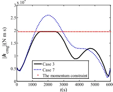
maxC , this constraint is inactive and the energy consumed will not be changed.The ZPM cases 3 and 7 in Table 2 were run. Case 7 is designed for the critical energy-optimal solution. In
Fig. 8, the momentum constraint of case 3 is active during the maneuver. The result for case 7 shows that the peak
momentum of the critical energy-optimal solution under the set maneuver time and boundary conditions is
C max
h
=2.5985!104 Nms. Figure 9 shows that the rate of momentum change constraint is not violated, and theprofiles are smooth. The energy performance metric for case 3 is E=1.2647!106N2m2s, and for case 7 is
E=1.1007!106N2m2s, which is the value of
e
C.0 1000 2000 3000 4000 5000 6000
0 0.5 1 1.5 2 2.5
3x 10
4 t(s) || h c m g ||( N m s ) Case 3 Case 7
The momentum constraint
Fig. 8 The angular momentum magnitude profiles of the CMGs
0 1000 2000 3000 4000 5000 6000
0 50 100 150 200 250 300 t(s) ||d h cm g
/dt
||
(N
m
) Case 3
Case 7
[image:19.595.199.383.387.537.2]The rate of momentum change constraint
Fig. 9 The rate of angular momentum change magnitude profiles of the CMGs
[image:19.595.195.385.567.714.2]The Pareto optimal front between the maneuver energy and the peak momentum was also computed by the
constraint method. Note that the final time is fixed at 6000s. Figure 10 shows the optimal front, together with the
momentum-optimal solution from case 1, the current optimal solution from case 3 and the critical
energy-optimal solution from case 7. As expected, the minimum maneuver energy decreases when the peak momentum
increases for a fixed
t
f. The front is bounded by the momentum-optimal solution and the critical energy-optimalsolution. The slope of the curve tends to infinity at the momentum-optimal solution and the slope is zero at the
critical energy-optimal solution.
1 1.5 2 2.5 3
x 104
0 2 4 6 8 10 12
14x 10
6
max(||hcmg||)(N m s)
E
(N
2 m 2 s)
Pareto optimal front Momentum-optimal solution Current energy-optimal solution Critical energy-optimal solution
t
[image:20.595.201.381.274.430.2]f=6000s
Fig. 10 The Pareto optimal front between maneuver energy and peak momentum
4.4 Maneuver Energy and Maneuver Time
For the ZPM energy-optimal control problem, it will be shown that the maneuver energy does not decrease
monotonically as the maneuver time increases, even under the ideal TEA final boundary condition. According to
Lemma 3.2, the sensitivity is
cmg
T T T T
cmg cmg
d
d d d
( ) ( )
d f d d d
f t
f t
e H
t t t t
à - · - · - - - Ô
Ä Õ
Å Ö
? ? h
h
w h w h . (27)
The augmented Hamiltonian
H
of the ZPM energy-optimal control problem is
*
+
*
+
cmg
T T T T
cmg cmg
T 2 T 2
p1 max p2 cmg cmg max
d
d d
: ( ) ( )
d d d
H
t t t
h h n n - · - · - - -- / - / ? h h
w h w h
w w h h
, (28)
and the resulting stationarity condition is
Two situations are now discussed, which depend on whether the rate of momentum change constraint is active
or not. If the rate of momentum change constraint at
t
f is active, then substituting the stationarity condition givenby (29) into (27), together with the ideal TEA final boundary condition, i.e. d dt tf
?0 and
*
( cmg)+
f
e
t
/ · J -h ?0, gives
T T 2
p1 max d
2 ( ) 2 ( )
d f f f f f f f
e
t h
t ? /u u - u ·h / n
, (30)
where uf is the abbreviation of u( )tf . Here, w is replaced by w? / ·u hcmg for simplicity. If the rate of momentum change constraint at
t
f is not active, then np1( )tf ?0, and henceT T
d
= 2 ( )
df f f f f f
e
t /u u - u ·h . (31)
In (30), since w ?hmax, it is straightforward to verify that
T T
2 ( ) 0
f f f f f
/u u - u ·h > using the data
given in Table 1. Thus, d 0 df
e
t > . In (31), the sign of
d d f
e
t cannot be determined. Thus, the energy performance can
also increase as the maneuver time increases. This is because the maintenance of the final angular momentum of the
CMGs still consumes energy, i.e. u? f·hf 0. The energy-optimal solution that satisfies
d =0 d f
e
t is defined as
the extremum energy-optimal solution.
In contrast, if we introduce a pseudo energy performance index given by
0
T
: tf d
t
E ?
Ð
w w t, (32)with the similar analysis as above, it may be proved that the optimal value of this performance index, denoted as
: min
e ? E, decreases when the maneuver time
t
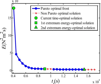
f increases under the ideal TEA final boundary condition.A set of ZPM energy-optimal problems with different fixed maneuver time was solved numerically to obtain
the relation curve between the minimum energy and maneuver time. Especially, the two ZPM cases 7 and 8 in Table
2 were used to seek possible extrema energy-optimal solutions. Figure 11 shows that the curve is not monotonic and
that the Pareto optimal front (the solid line) between the maneuver energy and maneuver time is discontinuous.
There are two extrema energy-optimal solutions. The first appears when the maneuver time is 9049.7s, with an
energy performance of 4.4340!105N2m2s. The second happens at 15358.5s with an energy performance of 2.3640!105N2m2s. Generally, the minimum energy decreases as the maneuver time increases. This occurs because in
(31), f
·
h
f is a small quantity, and thus d 0 dfe
t > holds for most of time. The relation between peak momentum
and maneuver time in the energy-optimal solutions is presented in Fig. 12. The curve is complex. It is shown that
before a maneuver time of 7500s the momentum magnitude threshold is reached, and then the peak momentum
keeps decreasing before the first extremum energy-optimal solution.
0.4 0.6 0.8 1 1.2 1.4 1.6
x 104 0
5 10 15
x 106
t f(s) E (N 2 m 2 s)
[image:22.595.205.380.212.357.2]Pareto optimal front Non Pareto optimal solution Current time-optimal solution 1st extremum energy-optimal solution 2nd extremum energy-optimal solution
Fig. 11 The Pareto optimal front between maneuver energy and maneuver time
0.4 0.6 0.8 1 1.2 1.4 1.6 1.8
x 104 0.8 1 1.2 1.4 1.6 1.8
2x 10
4 t f(s) m a x (| | h c m g ||)( N m s )
Results of numerical computations The momentum constraint Current time-optimal soltuion 1st extremum energy-optimal solution 2nd extremum energy-optimal solution
Fig. 12 The relation between peak momentum and maneuver time for the energy-optimal solutions
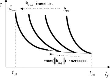
4.5 Synthesis of the ZPM MOP
As three objectives are involved in the ZPM MOP, the Pareto optimal front is a surface. The investigation
above was performed considering pairs of objectives, and the results will be synthesized in this subsection. In
practice, long maneuver times can cause problems for the space station power and thermal safety. The minimum
peak momentum and the minimum energy consumed change marginally when the maneuver time is near
t
me, which denotes the maneuver time of the first extremum energy-optimal solution. Denote the minimum maneuver time as [image:22.595.202.382.394.530.2]momentum magnitude parameter of the CMGs and
h
me be the peak momentum of the first extremum energy-optimal solution. For the ZPM mission with boundary conditions given in Table 1, two synthesized sketches, whichdescribe the relations among minimum maneuver energy, minimum peak momentum and maneuver time, are now
presented. They are also heuristic for other ZPM missions.
In Fig. 13, on each curve the maneuver time is fixed. The left end point and the right end point of each curve
represent the momentum-optimal solution and the critical energy-optimal solution, respectively. The Pareto solutions
located on the dashed line are not available under current CMGs capacity. In Fig. 14, on each curve the momentum
magnitude parameter of the CMGs is fixed. Along the thick lines the momentum constraint is active during the
maneuver, i.e. hmax= max
*
hcmg( )t+
;
along the thin line this constraint is not active, and the peak momentum decreases gradually. The left end points represent the time-optimal solutions under different momentum magnitude [image:23.595.200.399.361.496.2]parameters, while the rightmost point of intersection is the extremum energy-optimal solution.
Fig. 13 The variation in the Pareto front as the maneuver time varies
Fig. 14 The variation in the Pareto front as the maximum momentum varies
For the three types of ZPM paths, the energy-optimal path is the most favorable because of its smooth control
profile and energy-saving property. However, for practical flight, sufficient angular momentum redundancy of the
[image:23.595.208.388.537.668.2]CMGs is necessary. Figures 13 and 14 show the tradeoff relations among performance indices, and these may be
used for the compromise design of the ZPM path.
5 Conclusion
Three types of Zero Propellant Maneuver (ZPM) paths are considered: (i) momentum-optimal, (ii)
time-optimal and, (iii) energy-time-optimal. For the ZPM momentum-time-optimal control problem, the minimum peak momentum
of Control Momentum Gyroscopes (CMGs) is shown to decrease as the maneuver time increases under ideal Torque
Equilibrium Attitude (TEA) final boundary conditions. Indeed, the minimum peak momentum decreases as the
maneuver time increases under arbitrary fixed final boundary conditions. For the ZPM time-optimal control problem,
the minimum maneuver time decreases as the momentum magnitude parameter of the CMGs increases. For the ZPM
energy-optimal control problem, the minimum energy consumed will decrease if a larger CMGs momentum is
available. The minimum energy consumed does not monotonically decrease as the maneuver time increases, and
there could be several local extrema. However, the minimum energy generally decreases while the corresponding
peak momentum may change in a complex way. The Pareto optimal fronts between the peak momentum and the
maneuver time, and between the maneuver energy and the peak momentum are continuous, while the front between
the energy and the maneuver time is discontinuous.
Among the three path types, the typical ZPM momentum-optimal solution and time-optimal solution possess
the same structure, and they are singular. The energy-optimal path could save significant energy and the control
profile is smooth, and thus is a reasonable choice for the ZPM. For a specific ZPM case, the Multi-objective
Optimization Problem (MOP) is synthesized and conditioned simplified sketches of the Pareto optimal fronts are
presented. The sensitivity analysis method may be used to study the influence of parameter changes on the objective,
and applied to study the Pareto optimal front. By taking advantage of the properties of boundary conditions and KKT
multipliers, the first order sensitivity may be used to give insight into the solutions to the ZPM MOP.
The present paper uses heuristic methods, looking forward to a rigorous method. To this end, a promising
approach is the one proposed in [12], which is based on image space analysis and separation theorems. It is able to
find all the Pareto solutions and, overall, to optimize a scalar function over the Pareto set, without requiring to find it
explicitly. Due to its theoretical relevance, the latter approach is extremely interesting and will be studied in a
forthcoming paper.
References
1. Bedrossian, N., Bhatt, S., Lammers, M., Nguyen, L., Zhang, Y.: First ever flight demonstration of zero
propellant maneuver attitude control concept. In: 2007 AIAA GN&C Conference, Hilton Head, SC, USA,
AIAA 2007-6734 (2007)
2. Bedrossian, N., Bhatt, S., Lammers, M., Nguyen, L.: Zero propellant maneuver flight results for 180¡ ISS
rotation. In: 2007 International Symposium on Space Flight Dynamics, Annapolis, MD, USA,
NASA/CP-2007-214158 (2007)
3. Bedrossian, N., Bhatt, S., Kang W., Ross, I.M.: Zero-propellant maneuver guidance. IEEE Contr. Syst. Mag.
29(5), 53-73 (2009)
4. Bhatt, S.: Optimal reorientation of spacecraft using only control moment gyroscopes. Master’s thesis, Rice University, USA (2007)
5. Zitzler, E.: Evolutionary algorithms for multiobjective optimization: methods and applications. Ph.D.
dissertation, Swiss Federal Institute of Technology Zurich, Swiss (1999)
6. Rao, A.V., Benson, D.A., Darby C.L., Patterson, M.A., Francolin, C., Sanders, I., Huntington, G.T.: GPOPS: a
MATLAB software for solving multiple-phase optimal control problems using the gauss pseudospectral
method. ACM T. Math. Software 37(2), 1-39 (2010)
7. Garg, D., Patterson, M.A., Hager, W.W., Rao, A.V., Benson, D.A., Huntington, G.T.: A unified framework for
the numerical solution of optimal control problems using pseudospectral methods. Automatica 46(11),
1843-1851 (2010)
8. Schaub, H., Junkins, J.L.: Stereographic orientation parameters or attitude dynamics a generalization of the
rodrigues parameters. J. Astronaut. Sci. 44(1), 1-19 (1996)
9. Rehbock, V., Teo, K.L., Jennings, L.S.: A computational procedure for suboptimal robust controls. Dynam.
Control 2, 331-348 (1992)
10. Pesch, H.J.: The accessory minimum problem and its importance for the numerical computation of closed-loop
controls. In: Proceedings of the 29th IEEE Conference on Decision and Control, Honolulu, Hawaii, USA. pp.
952–953 (1990)
11. Hartl, R.F., Sethi, S.P., Vickson, R.G.: A survey of the maximum principles for optimal control problems with
state constraint. SIAM Rev. 37(2), 181-218 (1995)
12. Giannessi, F., Mastroeni, G., Pellegrini, L.: On the theory of vector optimization and variational inequalities.
image space analysis and separation. In: Giannessi, F. (eds.): Vector Variational Inequalities and Vector
Equilibria.Mathematical Theories, Series Nonconvex Optimization and its Applications, Vol.38, pp.141-215.
Kluwer, Dordrecht (2000)
Tables
Table 1 The initial and final boundary conditions for the ZPM mission
Initial state Value Final state Value
0 [0.1352, -0.4144, 0.5742]
T
!10-1 f [-0.3636, -0.2063, -4.1360]
T
!10-1
0(rad/s) [-0.2541, -1.1145, 0.0826]
T
!10-3 f(rad/s) [1.1353, 0.0030, -0.1571]T!10-3
0
h
(Nms) [-672.4768, -237.2650, -5276.7736]Tf
[image:27.595.88.523.268.446.2]h
(Nms) [-12.2022, -4822.5806, -183.0330]TTable 2 The designed ZPM path planning cases
Case Path type Final time
t
f (s) Momentum magnitudeparameter
h
max(Nms) Initialt
f(s)1 Momentum-optimal 6000 Minimize
h
max Not applicable2 Time-optimal Minimize
t
f 1.9524!104 13 Energy-optimal 6000 1.9524!104 Not applicable
4 Momentum-optimal 9000 Minimize
h
max Not applicable5 Time-optimal Minimize
t
f 5.3427!103 16 Time-optimal Minimize
t
f Infinity 17 Energy-optimal 6000 Infinity Not applicable
8 Energy-optimal Free 1.9524!104 1
9 Energy-optimal Free 1.9524!104 15000
Table 3 Results of the three optimal solutions
Case Path type Maneuver time (s) Peak momentum of the
CMGs(Nms)
Maneuver Energy
(N2m2s)
1 Momentum-optimal 6000 1.0618!104 1.2192!107
2 Time-optimal 4099.9 1.9524!104 1.7854!107
3 Energy-optimal 6000 1.9524!104 1.2647!106
[image:27.595.86.527.490.575.2]0 2000 4000 6000
−0.05
0 0.05 0.1 0.15
t(s)
σ 1
0 2000 4000 6000
−0.06
−0.04
−0.02
0
t(s)
σ 2
0 2000 4000 6000
−0.6
−0.4
−0.2
0
t(s)
σ 3
0 2000 4000 6000
−5
0 5 10 15x 10
−4
t(s)
ω x
(ra
d/
s)
0 2000 4000 6000
−15
−10
−5
0 5x 10
−4
t(s)
ω y
(ra
d/
s)
0 2000 4000 6000
−10
−5
0 5x 10
−4
t(s)
ω z
(ra
d/
s)
1 2x 10
4
(N
m
s
)
1 2x 10
4
(N
m
s
)
1 2x 10
4
(N
m
s
)