This is a repository copy of
Contrasting imputation with a latent variable approach to
dealing with missing income in choice models
.
White Rose Research Online URL for this paper:
http://eprints.whiterose.ac.uk/84331/
Version: Accepted Version
Article:
Sanko, N, Hess, S, Dumont, J et al. (1 more author) (2014) Contrasting imputation with a
latent variable approach to dealing with missing income in choice models. Journal of
Choice Modelling, 12. 47 - 57. ISSN 1755-5345
https://doi.org/10.1016/j.jocm.2014.10.001
eprints@whiterose.ac.uk
Reuse
Unless indicated otherwise, fulltext items are protected by copyright with all rights reserved. The copyright exception in section 29 of the Copyright, Designs and Patents Act 1988 allows the making of a single copy solely for the purpose of non-commercial research or private study within the limits of fair dealing. The publisher or other rights-holder may allow further reproduction and re-use of this version - refer to the White Rose Research Online record for this item. Where records identify the publisher as the copyright holder, users can verify any specific terms of use on the publisher’s website.
Takedown
If you consider content in White Rose Research Online to be in breach of UK law, please notify us by
Contrasting imputation with a latent variable approach to dealing
with missing income in choice models
Nobuhiro Sanko∗ Stephane Hess† Jeffrey Dumont‡ Andrew Daly§
Abstract
Income is a key variable in many choice models. It is also one of the most salient examples of a variable affected by data problems. Issues with income arise as measurement errors in categorically captured income, correlation between stated income and unobserved variables, systematic over- or under-statement of income and missing income values for those who refuse to answer or do not know their (household) income. A common approach for dealing especially with missing income is to use imputation based on the relationship among those who report income between their stated income for reporters and their socio-demographic characteristics. A number of authors have also recently put forward a latent variable treatment of the issue, which has theoretical advantages over imputation, not least by drawing not just on data on stated income for reporters, but also choice behaviour of all respondents. We contrast this approach empirically with imputation as well as simpler approaches in two case studies, one with stated preference data and one with revealed preference data. Our findings suggest that, at least with the data at hand, the latent variable approach produces similar results to imputation, possibly an indication of non-reporters of income having similar income distributions from those who report it. But in other data sets the efficiency advantage over imputation could help in revealing issues in the complete and accurate reporting of income.
Keywords: latent variables; missing income; discrete choice; random heterogeneity
1
Introduction
Income is arguably the most important socio-demographic variable in terms of explaining deterministic heterogeneity across respondents in choice models, notably in terms of explaining variations in cost sensitivity. It is however also one of the most difficult measures to capture accurately. Surveys often suffer from high rates of non-reporting for income, primarily due to respondents refusing to provide this information but also due to an often non-trivial share of respondents indicating that their actual total income is not known to them. Rates of non-reporting tend to be lower when capturing income as a categorical (rather than continuous) variable, and especially when using broader intervals, but this inevitably leads to measurement error. In addition to missing income information for some respondents, there are also potential issues in terms of correlation between stated income and other unobserved factors, as well as systematic respondent caused error, for example in the form of under- or over-reporting.
The issues of measurement error and missing variables seem rarely to be addressed in practical choice modelling (withWalker et al. 2010 being one exception), although it is clear that such issues are likely
∗Graduate School of Business Administration, Kobe University and Institute for Transport Studies, University of Leeds,
sanko@kobe-u.ac.jp
†Institute for Transport Studies, University of Leeds, s.hess@its.leeds.ac.uk
to lead to higher error in a choice model and sometimes cause bias in parameter estimates. Hausman
(2001) draws attention to this issue, for both linear and non-linear models and for both right-side and left-side variables. He also suggests solutions based on previous work, though the approach of this paper is closer to that of Walker et al. (2010) than that ofHausman (2001). Implicitly, measurement error is often ignored in practice, with an assumption that its effects are captured in the error term of the model. This can be more serious if, as is probable, measurement error or non-reporting are correlated with the values - for example, we typically have wider income bands for higher incomes and people with low and high incomes are believed to report less often than those with moderate incomes. Correlation with other unobserved factors potentially causes endogeneity bias, while systematic error could also lead to biased estimates. If a respondent purposefully misrepresents reality, for example by over- or under-stating key variables that are used in model estimation, then this is likely to have a detrimental effect on model results. Income may well be the most likely attribute to be affected by this problem. With the growing reliance on random coefficients models, there is also a risk that error in measured attributes is captured in the form of taste heterogeneity, potentially leading to biased results. Studies that analyse measurement errors include Walker et al. (2010), who introduced latent level-of-service variables to account for reported level-of-level-of-service variables with measurement error. Correlation with other unobserved factors can cause bias, and despite important work by for example Petrin and Train (2010) and Guevara and Ben-Akiva (2010), many studies still ignore the potential risk of such correlation, especially when it concerns explanatory variables in revealed preference (RP) data.
With income, the main focus in practical work has been on the treatment of missing income. A still all too common approach is to remove affected respondents from the data, which obviously leads to an undesirable reduction in sample size, can make the resulting dataset less representative of the real population, and cause endogeneity issues because of self selection. These factors all have implications both in terms of computing willingness-to-pay (WTP) measures as well as in forecasting. A crude approach is to place non-reporters at the sample-level mean income for reporters, but this assumption may not be justified and it is safer to estimate a separate cost coefficient for non-reporters. This allows a model to show whether non-reporters have higher (or lower) than average cost sensitivity, implying lower (or higher) than average income. Although this approach allows non-reporters to be incorporated in sample-level calculations of WTP measures, problems arise in forecasting, primarily as it becomes difficult to formulate the impact of income changes at the sample-level, given the special treatment for non-reporters.
An alternative is to attempt to impute the concerned attribute for those respondents with missing information, a process that essentially links the values for those respondents where the attribute is observed to other measured attributes (e.g. income linked to age) and then uses that relationship to infer the value for those respondents with missing data (e.g. Jiang and Morikawa, 2007). A key limitation of imputation is that it assumes that the relationship between the affected variable and the various other attributes used as explanators is the same across those respondents who report values and those who do not. Furthermore, when a value is imputed, it comes with imputation error and this needs to be taken into account in estimation to avoid biasing (towards zero) of the relevant coefficient, previously treated analytically byDaly and Zachary (1977) or by ‘multiple imputation’ byRubin(1987) andBrownstone and Steimetz (2005).
income for reporters as error free measures, when in reality, this will not be appropriate, especially when income is captured as a categorical variable.
In recent years, a number of applications have put forward the treatment of income as a latent variable, notably in the examples of the BIOGEME software (Bierlaire, 2003, 2005) and in Bolduc and Alvarez-Daziano (2010). This leads to the use of a hybrid model framework, an approach that is becoming increasingly popular in a number of disciplines, including transport (see e.g.Ben-Akiva et al.,
1999,2002a,b;Ashok et al.,2002;Bolduc et al.,2005). The key concept is that the variable of interest is considered as being unobserved, with only indicators thereof being captured in the data. A structural equation is employed to characterise the latent variable, and this is used to explain both the values of the indicators and the role of the latent component in the choice model. The models are used primarily for accommodating attitudes and perceptions, but have also been used to accommodate other behavioural phenomena such as the formation of plans leading to choices (Choudhury et al.,2010), or the treatment of level-of-service (Walker et al., 2010), preferred arrival time (Brey and Walker, 2011) and budgets (Dumont et al.,2013) as latent variables.
The use of hybrid models in the present context relies on formulating a single latent variable that represents a continuous income measure, which is a function of a number of other socio-demographic characteristics as well as a random disturbance. This latent income variable is then used to explain the stated income for those respondents who reported it and is also used as a measure of income inside the utility functions of the choice model, for example to explain variations in cost sensitivity.
The hybrid approach has a number of potential key advantages over the alternative methods dis-cussed above. In common with using imputation, the models are directly applicable for computing WTP distributions for the entire sample and also for using all respondents in forecasting, given that an income variable is now available for every decision maker. In contrast with imputation, the hybrid model however no longer treats stated income as an error-free measure of real income, potentially giving it an advantage in terms of accommdating measurement error. Furthermore, as stated income is no longer used as an explanatory variable in the choice model, potential issues with endogeneity bias due to correlation with other factors disappear. With imputation, this is often not the case as many studies use the imputed values only for non-reporters, retaining stated income for reporters. This potentially also leads to differences in error across these two groups. On the other hand, using the imputed values also for reporters means using a less accurate measure of income. Previous work by Bhat (1994) has avoided this issue by imputing a continuous income variable from categorical income data for all respon-dents, some of them with missing income. The difference in our work is that we use joint estimation with the choice model, meaning that the latent income variable is informed not just by the observed income levels (i.e. non-missing) but also by the choice behaviour in the data. Nevertheless, the hybrid model does continue to rely, like imputation, on the assumption that the structural relationship between socio-demographic variables and latent income is the same for reporters and non-reporters. Crucially however, in the hybrid model, the observed choices for non-reporters also contribute to the calibration of the latent income variable. This is in contrast with imputation, which uses no information from non-reporters. This, in conjunction with the error term in the structural equation for latent equation, also allows for under- or over-statement in reported values for specific respondents.
Bolduc and Alvarez-Daziano (2010) were concerned only with measurement error rather than missing income. Additionally, we produce empirical results from two case studies, one on stated preference (SP) data, and one on revealed preference (RP) data.
The remainder of this paper is organised as follows. The following section discusses modelling methodology. This is followed in Sections3 and4by the two separate empirical examples, and Section
5 summarises the findings and presents our conclusions.
2
Methodology
In a utility maximising framework, let the utility for alternative i in choice situation t for respondent
n be given by Uint = Vint+εint, where the deterministic component Vint is a function of measured
attributes xint, measured or reported socio-demographic characteristics zn, and estimated parameters β and κ. A general specification is given by Vint = f(β, κ, xint, zn), where β captures the impact of xint onVint, and where these sensitivities can vary as a function of zn, whereκ determines the impact
of zn. The remaining random component of utility is defined as εint.
Let us now assume that a given element in zn, say znk, is subject to the issues discussed in the
introduction, in particular missing values. We now use a latent variable αnk, defined by a structural
equation as:
αnk =f(γ, z∗n) +ηnk, (1)
wherez∗n=zn\znk, i.e. zn∗ is the subset which includes all variables inznexcept for znk. The random
componentηnk follows a standard Normal distribution and is independent ofzn∗. The functional form for f()is left to the analyst, and empirical evidence needs to be used to determine which components ofz∗n
should enter into the structural equation. This is a crucial part of the process of using such a model, and while a priori expectations could be helpful, a detailed empirical exploration of the relationship between socio-demographics and the variable of interest, i.e. znk, is needed in the specification search.
Inside our choice model, we now replaceznkbyαnk, possibly with additional function transformations
such aseαnk to ensure a positive sign for the attribute. We retainκas a vector of parameters associated
with socio-demographic attributes other than znk, and introduce τk as a new parameter associated
specifically with the latent variableαnk. We then have that the probability of the observed sequence of
choices for personnis given by:
P Cn(xn, z∗n, αnk, β, κ, τk) = T Y
t=1
P Cnt(xnt, zn∗, αnk, β, κ, τk), (2)
where P Cnt is the probability of the choice made by respondent nin task t, which will typically be of
logit form. P Cnt is a function of observed attributesxnt and zn∗, estimated parametersβ,κ and τk as
well as a specific realisation of the latent variable αnk. The vector of taste parameters β may follow a
random distribution across respondents with parameter vector Ωβ, say β ∼ h(β |Ωβ), in which case
we have that:
P Cn(xn, z∗n, αnk,Ωβ, κ, τk) = Z
β T Y
t=1
again conditional on a given realisation of the latent variable αnk. Thus far, our specification does
not make use of any additional information, and simply replaces znk by a construct composed of
a deterministic component and a random component, where this deterministic component would be informed only by the choices observed in the data. This is in contrast with imputation, where it is informed only by the values forzk for reporters and the values ofz∗ for all respondents.
In our case, additional model components are now used to helpinformthe role of the latent variable. At a bare minimum, we would have a single indicator (I) for each latent variable, which would be given by the original value for znk. The aim of the measurement component of the model is to explain the
observed value for that indicator on the basis of the latent variable αnk, where the lack of a
one-to-one relationship is motivated by the errors in znk. Furthermore, a special approach is needed for any
respondents for whom znk is not observed - for these respondents, the latent variable αnk does not
need to be used to explain any reported values, and is used only in the choice model component above (Equation3). The contribution by such respondents to the likelihood of the measurement model is thus set to unity, which goes to zero when working with the log-likelihood in estimation. In summary, we thus have:
P In(znk) =g(αnk, ζIk), ifznk is observed/reported (4)
P In(znk) = 1, ifznk is missing, (5)
where ζIk is a vector of estimated parameters, and where, as noted above, Equation 5 ensures that
missing observations do not contribute to the estimation of the measurement component of the model. The specific functional form used forg(αnk, ζIk)depends on the nature ofznk, which could for example
be continuous or ordinal.
Another point to note relates to the measurement scale of αnk. This latent variable incorporates a
standard normal random disturbance and as such has a domain going from negative to positive infinity. This is of course different from the units of the variableznk which it seeks to replace in the models. Let
us consider the specific case ofznk as being income, and specifically a case whereznk is measured in£.
Adding10units toαnk would not be expected to have the same impact as adding£10toznk, not least
as there would not be expected to be a one-to-one relationship betweenαnk andznk. However, ifαnk
performs well in proxying forznk, then a10%increase in αnk could be interpreted as a10%increase in
income.
As highlighted above, both model components (P CnandP In) are a function of a specific realisation
of the latent variable, and integration over the random component in αnk is thus needed. We use a
simultaneous specification, where the contribution by respondentnto the overall likelihood is given by:
Ln= Z
β Z
αnk
T Y
t=1
P Cnt(xnt, z∗n, αnk, β, κ, τk)P In(znk)h(β|Ωβ)φ(αnk) dαnkdβ, (6)
3
First case study
The data for the first case study comes from a stated choice survey for intra-mode commuter choices, using rail or bus (seeHess et al.,2012, for a full description). Respondents were faced with ten tasks each involving the choice between three alternatives, of which the first was a reference trip, with attributes held invariant across tasks. Alternatives were described by travel time, fare, the rate of crowding (0 to
1), the rate of delays (0to 1), the average delay across delayed trips, and the availability of a free text message (sms) delay information service. A sample of 368respondents was obtained from an internet panel, leading to 3,680observations in the data. Income was captured in 9 separate categories, with
12.5%missing from the final sample.
The estimation results for the first case study are summarised in Table1. Four models were estimated in the analysis, all of them allowing for random heterogeneity in the sensitivities to the six attributes, using Lognormal distributions (with µ and σ giving means and standard deviations for the underlying Normal distributions of the logarithms of the parameters), with a linear in attributes specification1, and with constants for the first two alternatives (δ1andδ2). All models were coded and estimated in Ox 6.2
(Doornik,2001), making use of Modified Latin Hypercube Sampling (MLHS) draws (Hess et al.,2006) for the random component, with simultaneous estimation of both model components for the hybrid structure in Equation6, and computing robust standard errors using the sandwich method.
In the first Mixed Logit (MMNL) model, labelled MMNL (mean), we use the category midpoints as continuous income measures for reporters, and replace the missing income for non-reporters by the sample-level average of reporters. In this model, the fare sensitivity for respondent n is multiplied by
incn
inc κinc
, where incn is the income for respondent n, inc is the sample mean income, and κinc is
an estimated income elasticity for the cost sensitivity. The estimates for this model show significant levels of heterogeneity for all six attributes, along with a significant negative income elasticity, showing decreasing cost sensitivity with increasing income.
The second model, MMNL (separate), moves away from the assumption that non-reporters are at the mean of the sample-level income distribution and instead estimates a separate fare coefficient for these respondents. We note that the model fit for this model is essentially indistinguishable from that of the first model, where the fit for non-reporters is slightly better, while that for reporters is slightly worse. The majority of parameters remain very similar between the two models. Importantly, we see that the mean (µ(ln(−βfare no inc.))) and standard deviation (σ(ln(−βfare no inc.))) for the fare
sensitivity for non-reporters (not interacted with any income data) are very similar to the base sensitivity for reporters (µ(ln(−βfare))andσ(ln(−βfare))). With the specific income specification used here, the base parameters relate to a respondent at the mean income (given that the multiplication byincn
inc κinc
then drops out), and this, along with the model fit observations, suggests that non-reporters in the present data are on average similar to reporters in terms of cost sensitivity. However, in this model, we see that the income effect for reporters suffers a substantial drop in significance.
We next move to a model using imputation of income on the basis of other socio-demographic variables. With a view to facilitating comparison with the later hybrid model, we use the imputed income values for both reporters and non-reporters, thus replacing the category midpoints for reporters. We also make use of the same structural equation for income in both models, with seven socio-demographic effects. Differences arise as in the sequential model (i.e. imputation), identification conditions mean that ηnk is omitted in the structural equation, and ζ is fixed to 1 in the measurement model. For
1The units for travel time and average delay are in minutes, those for fare are in£, the rates of crowding and delay are
the latter component, we use an ordered logit model to explain stated income for reporters, with eight estimated thresholds. We observe from the estimates for the structural model that stated income is higher for train users and male respondents, as well as increasing with the level of further education. Income is lower for respondents under 35 and higher for those who have a car available to them. The majority of parameters show only small differences between this model and the base MMNL structure. However, the effect of the imputed income variable,τinc, while negative, is not significant at the usual
levels of confidence. The overall log-likelihood for this model is given by the sum of the log-likelihoods of the sequentially estimated measurement model and choice model. We see that the fit of the choice model component is lower than in the base MMNL model, which uses the same number of parameters. A closer inspection shows that this is due to a reduction in the fit for the choices of reporters, which is not compensated by the improved fit for non-reporters, albeit that the latter change is bigger in relative terms. This suggests that imputed income is better than a sample-level mean for non-reporters, which is not surprising given that the former allows for differences in income across non-reporters. At the same time, the results suggest that imputed income provides inferior performance for reporters, which is not really surprising. The actual benefits will depend on the rate of non-reporting, which is low with the present data.
We finally turn our attention to the estimates for the hybrid model. This model uses the same specification for income as the imputation model, with the difference being the inclusion ofηnk, i.e. the
standard Normal disturbance in the structural equation forαn. Withαn now being used simultaneously
in both model components, we also estimateζ in the measurement model. The findings for the socio-demographic explanators of the latent income variable are consistent with those from the sequential model, though we see some variations in relative importance, and a sign change for γover55, which
however remains insignificant. The estimate for ζ is positive and significant, which, together with the increasing values for the thresholds, means that a higher value for the latent income variable leads to a higher probability for stated income to be in the higher categories (i.e. higher income). The core model parameters remain similar to those from the other three models, while the impact of the latent income variable on cost sensitivity (τinc) is negative and highly significant. The actual value remains
similar to that in the sequential model, but we are getting the benefit of a substantially reduced standard error, which also applies to the mean of the fare sensitivity, i.e. µ(ln(−βfare)). In terms of model fit,
the simultaneous estimation means that the total log-likelihood is no longer simply the sum of the two subcomponents, which are shown here conditional on the estimates. For the former, we maximised the log-likelihood for the two model components jointly where the latent income is shared with the same simulated disturbances by both components, while for the latter, the simulation was done separately, albeit with the same draws. We see that, with the same number of parameters, the fit to the choice data is slightly better than in the model using imputation, which is not surprising given that the hybrid model optimises the parameters in the structural equation for the latent variable to also explain the choices in the data. In common with the model using imputation, we see lower fit to reporters than when using the stated income, with higher fit for non-reporters than when using the sample-level mean income.
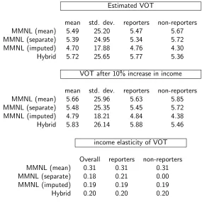
What is more surprising is the lower mean VOT in the model using imputation (18% lower than in the hybrid model), as well as reduced variation therein (30% lower than in the hybrid model), where this arguably partly relates to the use of the Lognormal distribution, where even small parameter differences can lead to large differences in VOT moments. On the other hand, the latter two models (imputed and hybrid) give a potentially more reasonable results in terms of showing higher VOT for reporters than non-reporters, assuming that it is more likely for non-reporters to have lower income.
The findings in terms of income elasticities are very similar at the overall level for all models except the first, which uses the mean income for non-reporters, where this seems to have an undue influence on leading to higher income elasticities, by a factor of 50% compared to the other models. For the second model, the income elasticity for non-reporters is zero as no income effect is used for these respondents. The similarity in the implied elasticities for reporters between the hybrid model and the second MMNL model suggests that percentage increases in the latent variable can be interpreted as percentage increases in income, in line with the comment at the end of Section 2.
Comparing these VOT income elasticities with external evidence, Daly and Fox (2012) review a number of sources and suggest an overall non-work value of around 0.3. The income elasticity of commuter time values in the UK is stated to be about 0.36 (DfT,2013, see para. 11.4.4), rather higher than the overall non-work value. While the values in our models are lower than the generally quoted ones, the sample is small and specific and the differences are not extreme.
4
Second case study
Our second case study makes use of revealed preference data from a survey for car ownership in Japan. The data come from the Japanese General Social Survey 2005 (JGSS-2005) collected in Japan in 2005, which is a part of the JGSS series started in 2000. The survey area covers all of Japan, and the sample includes respondents aged between 20 and 89. The interview collects information including gender and age of all household members, car ownership and income (19categories) at a household level, occupation and education for the respondent and his/her spouse, and various others. For the present study, we made use of a sample of 1,668 respondents who provided information on car ownership. Out of this sample, income was missing for 614respondents, i.e. a very substantial36.8%of the sample.
We estimated four models using a similar approach to that used in the first case study, with the difference being that the choice model is now a binary probit (BP) model. The dependent variable is a binary indicator for whether a household owns a car or not, meaning that we estimate a single threshold in the model. In each model, we explain the utility of car ownership by seven variables other than income, relating to household composition as well as residential location. In all models, income, whether stated, imputed or latent, enters the utility in a linear form. The estimation results are summarised in Table3. The first model, BP (mean), replaces missing income by the sample-level mean for reporters. We observe that increases in household size lead to increased probability of owning cars, where this effect is stronger for the number of male household members. The number of household members aged 18
no surprise that this second model produces very similar parameters from the first model, along with essentially identical model fit.
Turning to the BP model with imputed income for all respondents, we see a higher log-likelihood for the choice model compared to the first model, with the same number of parameters. This is due to larger improvement in the ability to explain the choices for non-reporters which far exceeds the loss in explanatory power in explaining the choices of reporters. We note small changes in the estimates for the socio-demographic terms within the BP model, along with a more significant estimate for the income parameter. In the measurement model which is used to calculate the imputed income, we use an ordered probit (OP) model with18 thresholds. Turning to the structural equation, the imputed income is explained by characteristics of the respondent and his/her spouse2. The respondent is either male without wife, female without husband, or male or female with his/her spouse, so only two constants are included. Note that unmarried male and female respondents also are termed husband and wife respectively in this case study. The effects of working, alone and in interaction with age are examined; the former is statistically significant for only wives, while the latter is statistically significant only for husbands. Both high school and university education lead to higher income, and the effect of the latter is larger (base is no high school education). Working hours have an impact on income especially for wives. Employment status is statistically significant only for husbands, with the highest effect for executives, followed by department head and section head (the base is lower than the section head level). Income is also higher for husbands employed in large companies or government agencies compared to those in smaller companies. Husbands employed in finance/insurance industries have higher income compared to other industries. In summary, a husband’s pay depends on the type of employment and experience, while a wife’s pay depends more on the hours worked, with less variance in hourly rates (strong per-hour effect).
The findings from the hybrid model are again very comparable to those from the model using imputation, albeit that we see small additional gains in log-likelihood in the choice model, which is to be expected given the simultaneous estimation. The estimates in the structural equation are, overall, similar to those from the third model, with small changes in relative importance. In the measurement model, we see that, as latent income increases, so does the probability of higher stated income (higher category), given the positive estimate for ζ. It can also be noted that, in line with the theoretical advantages in terms of efficiency compared to the third model, we note a slightly lower standard error for τinc (0.069compared to0.075).
In this data, in contrast to the first case study, it is not possible to compute measures of willingness to pay because of the absence of attributes relating to the alternatives. However, it is possible to calculate an income elasticity of car ownership to allow quantitative comparisons to be made between the outputs of the alternative models. The results from these calculations are summarised in Table43.
A key finding here is that the elasticities for reporters are higher with imputation than in the model using mean income and in the hybrid model, while the model using mean income underestimates the gap in income elasticity between reporters and non-reporters compared to the final two models. The model with separate coefficients is not able to provide an elasticity for the non-reporters, while the elasticities for non-reporters are higher in the model using imputation than in the hybrid model. It can of course be noted that the differences across models are small, and that while the elasticities in the hybrid model are
2Detailed socio-demographic information is available for only the respondent and his/her spouse, although car ownership
is explained by characteristics of all household members. Investigation of which variables should appear in each of the submodels is a task for further research.
lower than in the model using imputation, the differences may not be significant, and the relationship between the two groups of respondents (reported and non-reporters) is the same. Finally, overall, the elasticity might appear low, but it must be remembered that this is the elasticity for having one or more cars, not total car ownership, in a market where86% of the households have cars.
5
Conclusions
This paper has contrasted the use of imputation with the treatment of income as a latent variable in a choice model context. The motivation for such an approach is that stated income is affected by a number of key issues, in the form of measurement error (e.g. due to being measured in categories), missing observations, correlation with other unobserved factors, and bias introduced by the respondent in the form of under or overstated income. Missing income especially has received attention in practical work.
In a hybrid framework, the latent income variable is then used inside the choice model as well as being an explanator in a measurement model used to explain stated income. It has a deterministic as well as a random component, where the former explains latent income as a function of other respondent characteristics, much as in imputation. Unlike a method relying directly on stated income, this approach has the advantage of making provision for error in the respondent’s reported income. By treating stated income as a dependent rather than explanatory variable, it also avoids issues with endogeneity bias. In comparison with using imputation for missing income information, the method has the theoretical advantage that the latent income variable is informed not just by the relationship between observed income (i.e. for those respondents who provide it) and other socio-demographic characteristics, but also by the choices made by all respondents. In common with imputation, the method is directly applicable for forecasting without the need to eliminate a share of respondents who did not provide income information.
Our empirical tests on two datasets, one from a stated preference survey and one from a revealed preference survey, show that the hybrid approach is able to explain the choices of non-reporters better than is the case for a model relying on either using the mean income or a separate coefficient for such respondents. However, this comes at the expense of reducing the explanatory power on the data for those respondents who did report income. The benefits of the hybrid approach thus depend partly on the rate of non-reporting in the sample. The approach clearly retains theoretical advantages in terms of endogeneity bias and measurement error, but the practical implications of this seem limited in the present case. Moreover, the findings we obtain by using imputed income are very similar to those from the hybrid model, notwithstanding differences in elasticities of around13.6%to 16.8%in the Japanese data. A possible reason for our findings is that the behaviour of non-reporters is in line with that of reporters, and this is supported by the findings from the models estimating separate effects related to income for the two groups.
its theoretical advantages and elegant treatment of the issue, a clearer picture of the actual benefits is required to warrant its use in practical work.
Acknowledgements
The Japanese General Social Surveys (JGSS) are designed and carried out at the Institute of Regional Studies at Osaka University of Commerce in collaboration with the Institute of Social Science at the University of Tokyo under the direction of Ichiro TANIOKA, Michio NITTA, Noriko IWAI and Tokio YASUDA. The project is financially assisted by Gakujutsu Frontier Grant from the Japanese Ministry of Education, Culture, Sports, Science and Technology for 1999-2008 academic years, and the datasets are compiled and distributed by SSJ Data Archive, Information Center for Social Science Research on Japan, Institute of Social Science, the University of Tokyo. The first author acknowledges the financial support from a Grant-in-Aid for Scientific Research (Grant Nos. 22730334, 24330132 and 25380564) from the Japan Society for the Promotion of Science.
References
Ashok, K., Dillon, W. R., Yuan, S., 2002. Extending discrete choice models to incorporate attitudinal and other latent variables. Journal of Marketing Research, 31–46.
Ben-Akiva, M., Walker, J., Bernardino, A., Gopinath, D., Morikawa, T., Polydoropoulou, A., 2002a. Integration of choice and latent variable models. In: Mahmassani, H. (Ed.), In Perpetual motion: Travel behaviour research opportunities and application challenges. Pergamon, Ch. 13, pp. 431–470.
Ben-Akiva, M., Walker, J., McFadden, D., G¨arling, T., Gopinath, D., Bolduc, D., B¨orsch-Supan, A., Delqui´e, P., Larichev, O., Morikawa, T., Polydoropoulou, A., Rao, V., 1999. Extended framework for modeling choice behavior. Marketing Letters 10 (3), 187–203.
Ben-Akiva, M., Walker, J., McFadden, D., Train, K., Bhat, C. R., Bierlaire, M., Bolduc, D., Boersch-Supan, A., Brownstone, D., Bunch, D. S., Daly, A., de Palma, A., Gopinath, D., Karlstrom, A., Munizaga, M. A., 2002b. Hybrid choice models: Progress and challenges. Marketing Letters 13 (3), 163–175.
Bhat, C., 1994. Imputing a continuous income variable from grouped and missing income observations. Economics Letters 46, 311–319.
Bierlaire, M., 2003. BIOGEME: a free package for the estimation of discrete choice models. Proceedings of the 3rd Swiss Transport Research Conference, Monte Verit`a, Ascona.
Bierlaire, M., 2005. An introduction to BIOGEME Version 1.4. biogeme.epfl.ch.
Bolduc, D., Alvarez-Daziano, R., 2010. On estimation of hybrid choice models. In: Hess, S., Daly, A. (Eds.), Choice Modelling: The State-of-the-Art and the State-of-Practice: Proceedings from the Inaugural International Choice Modelling Conference. Emerald Group Publishing, pp. 259–288.
Brey, R., Walker, J., 2011. Latent temporal preferences: An application to airline travel. Transportation Research Part A 45 (9), 880–895.
Brownstone, D., Steimetz, S., 2005. Estimating commuters vot with noisy data. Transportation Research Part B 39 (10), 865–889.
Choudhury, C., Ben-Akiva, M., Abou-Zeid, M., 2010. Dynamic latent plan models. Journal of Choice Modelling 3 (2), 50–70.
Daly, A., Fox, J., 2012. Forecasting mode and destination choice responses to income change. paper presented at the 13th International Conference on Travel Behaviour Research, Toronto.
Daly, A., Zachary, S., 1977. The Effect of Free Public Transport on The Journey to Work. Transport and Road Research Laboratory Report SR388.
DfT, 2013. Transport analysis guidance, unit 3.12.2, modelling road pricing, draft, accessed 29 october 2013. UK Department for Transport.
Doornik, J. A., 2001. Ox: An Object-Oriented Matrix Language. Timberlake Consultants Press, London.
Dumont, J., Hess, S., Daly, A., Ferdous, N., 2013. The use of the multiple discrete continuous extreme value modeling framework when the budget is latent: two consumer package good examples. paper presented at the 3rd International Choice Modelling Conference, Sydney.
Guevara, C. A., Ben-Akiva, M., 2010. Addressing endogeneity in discrete choice models: Assessing control-function and latent-variable methods. In: Hess, S., Daly, A. (Eds.), Choice Modelling: The State-of-the Art and the State-of-practice; Proceedings from the Inaugural International Choice Mod-elling Conference. Emerald Group Publishing, pp. 353–371.
Hausman, J., 2001. Mismeasured variables in econometric analysis: problems from the right and prob-lems from the left. The Journal of Economic Perspectives 15 (4), 57–67.
Hess, S., Stathopoulos, A., Daly, A. J., 2012. Allowing for heterogeneous decision rules in discrete choice models: an approach and four case studies. Transportation 39 (3), 565–591.
Hess, S., Train, K., Polak, J. W., 2006. On the use of a Modified Latin Hypercube Sampling (MLHS) method in the estimation of a Mixed Logit model for vehicle choice. Transportation Research Part B 40 (2), 147–163.
Jiang, M., Morikawa, T., 2007. Measuring value of travel time savings with resource value and com-modity value. Doboku Gakkai Ronbunshuu D 63 (3), 302–310.
Petrin, A., Train, K., 2010. A control function approach to endogeneity in consumer choice models,. Journal of Marketing Research 47 (1), 3–13.
Rubin, D. B., 1987. Multiple imputation for nonresponse in surveys. Vol. 307. Wiley.
Table 1: Estimation results for first case study
MMNL (mean) MMNL (separate) MMNL (imputed) Hybrid
Total LL -2,989.99 -2,989.58 -3,577.80 -3,583.58
LL (Measurement) - - -583.50 -591.46
LL (Choice) -2,989.99 -2,989.58 -2,994.31 -2,992.89 LL (Choice, non-reporters) -361.88 -360.74 -359.70 -359.39
LL(Choice, reporters) -2,628.11 -2,628.84 -2,634.61 -2,633.50
est. t-rat. est. t-rat. est. t-rat. est. t-rat.
δ1 0.8026 9.87 0.8032 9.87 0.7955 9.81 0.7871 9.77
δ2 0.3264 4.36 0.3250 4.29 0.3442 4.67 0.3353 4.53
µ(ln(−βtravel time)) -2.7296 -20.71 -2.7390 -20.26 -2.6704 -21.52 -2.6521 -24.31
µ(ln(−βfare)) 1.1914 11.77 1.1761 9.92 1.3555 11.08 1.4168 14.77
µ(ln(−βfare no inc.)) - 1.2961 8.35 -
-µ(ln(−βcrowding)) 0.7778 3.78 0.6787 2.93 0.8487 3.53 0.6727 2.52
µ(ln(−βrate of delays)) 1.0260 6.06 1.0148 6.15 1.0433 6.83 1.0375 6.40
µ(ln(−βav. delay)) -3.5713 -8.40 -3.5564 -8.16 -3.7148 -7.62 -3.2219 -10.76
µ(ln(βdelay sms)) -0.9986 -4.37 -1.0362 -4.72 -1.2043 -4.52 -1.0562 -5.53
σ(ln(−βtravel time)) 0.9606 7.03 0.9755 7.92 0.8304 6.28 0.8389 8.52
σ(ln(−βfare)) 1.4885 11.32 1.4519 15.60 1.4340 13.36 1.5359 12.29
σ(ln(−βfare no inc.)) - 1.5550 8.58 -
-σ(ln(−βcrowding)) 1.3801 10.02 1.4792 9.42 1.5110 13.31 1.8602 6.35
σ(ln(−βrate of delays)) 1.2645 10.84 1.3362 10.98 1.1138 8.94 1.0265 10.13
σ(ln(−βav. delay)) 1.7719 9.85 1.7574 10.00 2.1121 7.46 1.2939 9.86
σ(ln(βdelay sms)) 1.0396 6.51 1.0932 7.44 1.2837 9.31 1.1238 11.56
κinc -0.3135 -2.86 -0.2070 -1.67 -
-τinc - - -0.1909 -1.38 -0.2015 -2.85
γtrain - - 0.9656 4.41 0.6624 3.71
γf emale - - -0.6759 -3.17 -0.5056 -3.09
γundegraduate - - 0.7627 3.10 0.8559 4.41
γpostgrad. - - 1.9081 6.67 1.2476 6.30
γunder35 - - -0.9725 -4.37 -0.3598 -2.46
γover55 - - -0.2269 -0.80 0.1916 1.39
γcaravailable - - 0.6802 3.19 0.7786 5.35
ζ - - 1 - 0.6152 2.39
threshold1 - - -3.2221 -9.02 -2.0353 -5.56
threshold2 - - -1.7065 -6.14 -0.4994 -1.57
threshold3 - - -0.7744 -2.86 0.4816 1.38
threshold4 - - 0.2026 0.75 1.6090 3.58
threshold5 - - 1.6960 5.79 3.8471 4.44
threshold6 - - 2.5668 8.26 5.7575 4.16
threshold7 - - 3.5482 10.29 8.9055 3.94
Table 2: Implied VOT distributions and VOT income elasticities for first case study
Estimated VOT
mean std. dev. reporters non-reporters MMNL (mean) 5.49 25.20 5.47 5.67 MMNL (separate) 5.39 24.95 5.34 5.72 MMNL (imputed) 4.70 17.88 4.76 4.30 Hybrid 5.72 25.65 5.77 5.36
VOT after 10% increase in income
mean std. dev. reporters non-reporters MMNL (mean) 5.66 25.96 5.63 5.85 MMNL (separate) 5.48 25.35 5.45 5.72 MMNL (imputed) 4.79 18.21 4.84 4.38 Hybrid 5.83 26.14 5.88 5.46
income elasticity of VOT
Table 3: Estimation results for second case study
BP (mean) BP (separate) BP (imputed) Hybrid
LL (total) -446.68 -446.59 -2,983.88 -2,974.56
LL (Measurement) - - -2,544.12 -2,547.40
LL (Choice) -446.68 -446.59 -439.76 -438.67 LL (Choice, non-reporters) -142.55 -142.61 -134.06 -133.50 LL(Choice, reporters) -304.13 -303.98 -305.71 -305.17
est. t-rat. est. t-rat. est. t-rat. est. t-rat.
κnumber of males (-17yrs) in household 0.8544 4.56 0.8536 4.56 0.7374 4.15 0.7727 4.33
κnumber of males (18-yrs) in household 0.7823 7.65 0.7873 7.87 0.7578 8.48 0.7631 8.03
κnumber of females (-17yrs) in household 0.4900 4.06 0.4878 4.03 0.3440 2.90 0.3442 2.81
κnumber of females (18-yrs) in household 0.4858 5.76 0.4906 5.77 0.5272 6.42 0.5299 5.80
κTokyo’s 23 wards -1.2049 -6.48 -1.2031 -6.46 -1.2431 -6.79 -1.3389 -6.64
κYokohama/Kawasaki cities -0.8808 -2.85 -0.8727 -2.82 -0.7201 -2.33 -0.8456 -2.58
κOsaka city -1.4320 -3.69 -1.4387 -3.66 -1.1462 -3.00 -1.3992 -3.57
BP threshold 1.0296 6.64 1.0370 6.60 1.1160 7.24 1.1316 6.27
κannual household income (JPY 10 million) 1.2651 5.01 1.2910 4.54 -
-κmissing income - 0.7007 4.63 -
-τinc - - 0.5570 7.41 0.3908 5.66
γhusband in household - - 0.3517 2.65 0.5813 2.61
γwife in household - - 0.0651 0.48 0.0925 0.42
γwife working - - 0.2512 1.82 0.3917 1.75
γage of husband if he works - - 0.0050 2.40 0.0077 2.22
γhigh school education for husband - - 0.1766 1.63 0.2982 1.73
γhigh school education for wife - - 0.2786 2.67 0.4758 2.81
γuniversity education for husband - - 0.4404 3.53 0.6800 3.32
γuniversity education for wife - - 0.4987 4.17 0.7932 3.84
γworking hours per week for husband - - 0.0028 1.17 0.0072 1.79
γworking hours per week for wife - - 0.0108 2.91 0.0181 2.91
γhusband working as executive - - 1.1265 7.74 1.8531 5.97
γhusband working as department head - - 0.7474 5.56 1.1486 4.61
γhusband working as section head - - 0.4628 3.90 0.7442 3.60
γhusband working as large company employee - - 0.4339 5.15 0.6870 4.39
γhusband working as government employee - - 0.6159 5.53 1.0061 4.69
γhusband working in a financial institutions/insurance - - 0.6440 2.92 1.0446 3.05
ζ - - 1 - 0.7413 5.90
OP threshold1 - - -1.2389 -7.19 -1.5740 -6.81
OP threshold2 - - -0.7316 -4.75 -0.9451 -4.90
OP threshold3 - - -0.4169 -2.78 -0.5494 -3.02
OP threshold4 - - -0.1410 -0.95 -0.2024 -1.13
OP threshold5 - - 0.0054 0.04 -0.0184 -0.10
OP threshold6 - - 0.4693 3.08 0.5637 2.97
OP threshold7 - - 0.9857 6.23 1.2094 5.76
OP threshold8 - - 1.4347 8.79 1.7690 7.59
OP threshold9 - - 1.8043 10.76 2.2258 8.72
OP threshold10 - - 2.0922 12.20 2.5797 9.47
OP threshold11 - - 2.3771 13.51 2.9292 10.07
OP threshold12 - - 2.6279 14.57 3.2370 10.51
OP threshold13 - - 3.0454 16.05 3.7503 11.07
OP threshold14 - - 3.3694 17.02 4.1494 11.40
OP threshold15 - - 3.6647 17.81 4.5139 11.61
Table 4: Implied car ownership income elasticities for second case study
BP (mean) BP (separate) BP (imputed) Hybrid reporters 0.0930 0.0929 0.1112 0.0979 non-reporters 0.0876 - 0.0759 0.0650