Production flow analysis & inventory control for Orford Refrigeration

University of Southern Queensland

Faculty of Engineering and Surveying

Production Flow Analysis & Inventory Control for Orford

Refrigeration

A dissertation submitted by

Yip Soon YEW

In fulfillment of the requirements of

Course ENG4111 and 4112 Research Project

Towards the degree of

Bachelor of Engineering (Mechatronics)

Group technology is an important technique in the planning of manufacture that allows the advantages of flow production organization to be obtained in what otherwise would be jobbing of batch manufacture. The approach is to arrange separate machines groups with appropriate internal group layout to suit the production of specific component families, formed in accordance with the similarity of operations that to be performed on them.

Certification

I certainly that the ideas, designs and experimental work, results, analyses and

conclusions set out in this dissertation are entirely my own effort, except where otherwise indicated and acknowledge.

I further certify that the work is original and has not been previously submitted for assessment in any other course or institution, except where specifically stated.

YEW YIP SOON

Student Number: W0006618

Signature

Acknowledgements

Acknowledgements

I would like to take this opportunity to express my sincere appreciation towards my supervisor, Dr. Harry Ku for his valuable guidance and supervision throughout the course of my thesis. He has not only allowed me to explore my capabilities and skills, but also helped cultivate in me a keen interest in the area of manufacturing processes. It has been a truly memorable and beneficial experience to have him as my supervisor.

I would also like to show my appreciation towards Dr. Selvan Pather for his time and guidance during the course of my thesis. He has been an inspiration to me and given me many intellectual challenges to face. He also allowed me to expand my boundaries to where I would never have thought I could reach.

A very important and valued person whom without which the success of this research project would not have been possible is Mr Ian Otto, the Product Development Advisor of Orford Refrigeration. He has provided enormous amount of help, guidance and valuable information for this research project. He is a man of great patience and it has been wonderful to work with him. With all the support and valuable times he has given to me, he has indeed made this research project a great one to work on despite all odds.

I would also like to thank the following important Orford Refrigeration staffs members for their help and guidance.

Table of Contents

Abstract i

Disclaimer ii

Acknowledgement iii

Table of Content vi

List of Figures vii List of Tables ix

Appendices x Chapter 1 Introduction 1

Chapter 2 Literature Review 4

2.1 Background 4

2.2 Types of algorithm in GT 4

2.2.1 Array – based 4

2.2.2 Clustering 5

2.2.3 Mathematical programming 6

2.2.4 Graph Theoretic 7

2.3 Manufacturing application 8

2.4 Product application 10

2.5 Summary 11

Chapter 3 Basic principle of GT 12 3.1 Introduction 12

3.2 Part families 12

3.3 Visual inspection 14

3.4 Parts classification and coding 15

3.4.1 Features of Parts classification and coding 17

3.4.2 Opitz classification system 23

4.2 Grouping parts and machines by Rank Order Clustering 30

4.3 Direct Order Clustering 35

4.4 Arranging machines in GT cells 39

Chapter 5 Plant layout 42

5.1 The job shop layout 42

5.2 The line flow layout 43

5.3 The fixed position layout 45

5.4 Group technology layout 46

5.5 Orford Refrigeration machine shop layout 49

Chapter 6 Inventory control 51

6.1 Introduction 51

6.2 Periodic Reorder system 51

6.3 Reorder Point System 53

6.4 Economic Order Quantity 54

6.5 Orford Refrigeration inventory system 56

Chapter 7 Results and discussion 57

Reference 63

List of Figures

Figure 1.1: (b) Grouped parts 2

Figure 2.1 The machines in a formal machine cell are located in close 10 proximity to minimize part handling, throughput time, setup,

Figure 2.2 The database of existing parts is then scanned to find items with 11 identical or similar codes.

Figure 3.1 Part family may be grouped with respect to production 13 operations, that is, machine, processes, operations,

tooling, and etc.

Figure 3.2 Parts having similar design features such as geometric 14 shape, size, materials and etc.

Figure 3.3 Intuitive grouping or visual inspection for simple 15 part/process mixes.

Figure 3.4 Hierarchical structure. 19

Figure 3.5 Mixed – mode structure. 20

Figure 3.6 Basic structure of the Opitz system of parts classification 24 and coding.

Figure 4.1 First iteration in the Rank Order Clustering. 33 Figure 4.2 Second iteration in the Rank Order Clustering. 33 Figure 4.3 Third iteration in the Rank Order Clustering. 34 Figure 4.4 Fourth iteration in the Rank Order Clustering. 34 Figure 4.5 A part – machine groupings in the Rank Order Clustering. 35 Figure 4.6 First iteration in Direct Order Clustering. 36 Figure 4.7 (above) & Figure 4.8 (below) 2nd & 3rd iteration. 37 Figure 4.9 (above) & Figure 4.10 (below) 3rd &4th iteration. 37 Figure 4.11 Two groups of families have been formed. 39

Figure 5.1 Process type layout. 43

Figure 5.2 Product – specific layout. 45

Figure 5.3 A group technology layout. 47

Figure 5.4 U – shape machine layout. 48

Figure 5.5 Machine shop layout. 50

Figure 6.1. The basic function of stock (inventory) is to insulate 52 the production process from changes in the environment.

Figure 6.2. The periodic reorder system. 53

Figure 7.2 Another type of machine used for folding process. 59 Figure 7.3 Some example of the parts produced from sheet metal. 59

Figure 7.4 Outer back – upper. 60

Figure 7.5 Shelf support channel. 60

Figure 7.6 Castor plate – front. 61

Figure 7.7 TOM – type A. 61

Figure 7.8 Unit runner. 61

Figure 7.9 Global 2.0, a very high capacity punching machine. 62

Lists of Tables

Table 3.1 Design and Manufacturing Attributes typically included 18 in a Group Technology classification and coding system.

Table 3.2 Selected examples of worldwide classification and 21 coding systems.

Table 3.3 Possible code numbers indicating operation and/or 27 machines for sortation in PFA.

Table 3.4 PFA chart, also know as Part – Machine Incidence Matrix. 28

Table 4.1 From – To chart. (example) 40

Table 4.1a From and To sums: First Iteration. 41

Table 4.1b From and To sums: Second Iteration with 41 machine 3 removed.

Appendices

Appendix A Project Specification Appendix B Production Schedule Appendix C Parts Route Sheet Appendix D PFA Chart

1. Introduction

Manufacturing environments and production processes have changed substantially over the past two decades. Rather than producing as much possible with limited options, customer buying habits now require just in time delivery as well as more “made-to order” products. Customers are demanding the latest and greatest in technology before the new product is barely off the drawing board. In 1971, Opitz [1] related that at least 48% of all components designs produced each year are new. Today, that number is considered to be higher. In order to maintain profitability, companies must find ways to bring new products to market more expediently and cost effectively while engaging in continuously improving these products.

Recently, Cellular Manufacturing (CM) has emerged as a strong approach for improving operations in batch and job shop environments. In CM, Group Technology (GT) is used to form part families based on similar processing requirements. Parts and machines are then grouped together based on sequential or simultaneous techniques. This approach results in cells where machines are located in relative proximity based on processing requirements rather than similar functional aspects. Decision making and accountability are more locally focused, often resulting in quality and productivity improvements.

1. Introduction

harness resources for small lot production. However, unlike mass production lines used for large quantities of a single part, families of similar parts with similar processes are manufactured. Parts are grouped into families based on these similarities and produced in manufacturing cells where machines are dedicated to a particular family (shown in Figure 1.1a and 1.1b).

Figure 1.1: (a) Ungrouped parts Figure 1.1: (b) Grouped parts

Inventory control is needed in every organization. A typical manufacturing company holds 20% of its production as stock, and this has annual holdings costs of around 25% of value. All organizations, not just manufacturers, hold stocks of some kind and these represent a major investment which should be managed efficiently. If stocks are not controlled properly the costs can become excessive and reduce an organization’s ability to compete. Efficient inventory control then becomes a real factor in an organization’s long term survival.

Technology analysis, the first part of the analysis will be focus on the basic concept of Group technology. In this section, some of the technique such as Parts classification and Coding and also Production Flow Analysis will be discuss to show how to group parts together and to form parts families. After part families have been identified, the following section will be focus on how grouping the machines into a cells. Here, two common techniques will be illustrated which are Rank Order Clustering and Direct Clustering, and also what is the advantages and disadvantages of these techniques. In the last section of the first part of the thesis, methods like using a “From - To” chart to organize the machines into the most logical arrangement, and to maximizes the proportion of in – sequence moves will be discuss here.

2. Literature review

2. Literature Review

2.1 Background

Cellular manufacturing emerged as a production strategy capable of solving the problem of complexity and long manufacturing lead times in batch production systems in the beginning of the 1960s. Burbidge (1979) defined group technology (GT) as an approach to the optimization of work in which the organizational production units are relatively independent groups, each responsible for the production of a given family of products.

The fundamental problem in cellular manufacturing is the formation of product families and machine cells. The objective of this product-machine grouping problem is to form perfect (i.e. disjoint) groups in which products do not have to move from one cell to the other for processing.

2.2 Types of algorithms in GT

2.2.1 Array – based

Array-based clustering methods perform a series of column and row permutations to form product and machine cells simultaneously. King (1980) and later King and Nakornchai (1982) developed the earliest array-based methods. King and Nakornchai (1982), Chandrasekharan and Rajagopalan (1987), Khator and Irani (1987), and Kusiak and Chow (1987) proposed other algorithms. A comprehensive comparison of three array-based clustering techniques is given in Chu and Tsai (1990). The quality of the solution given by these methods depends on the initial configuration of the zero-one matrix.

2.2.2 Clustering

2. Literature review

Miltenburg and Zhang (1991) present a comprehensive comparison of nine clustering methods where non-hierarchical methods outperform both array-based and hierarchical methods.

2.2.3 Mathematical programming

based on an efficient p-median approach. Akturk and Turkcan (2000) propose an integrated algorithm that solves the machine/product grouping problem by simultaneously considering the within-cell layout problem. Plaquin and Pierreval (2000) propose an evolutionary algorithm for cell formation taking into account specific constraints. Zhao and Wu (2000) present a genetic algorithm for cell formation with multiple routes and objectives. Caux et al. (2000) address the cell formation problem with multiple process plans and capacity constraints using a simulated annealing approach. Onwubolu and Mutingi (2001) develop a genetic algorithm approach taking into account cell-load variation. Uddin and Shanker (2002) address a generalized grouping problem, where each part has more than one process route. The problem is formulated as an integer programming problem and a procedure based on a genetic algorithm is suggested as a solution methodology.

2.2.4 Graph theoretic

2. Literature review

fixed number of groups and with bounds on cell size. Their algorithm for grouping in flexible manufacturing systems is also applicable in the context of GT. Vannelli and Kumar (1986) developed graph theoretic models to determine machines to be duplicated so that a perfect block diagonal structure can, be obtained. Kumar and Vannelli (1987) developed a similar procedure for determining parts to be subcontracted in order to obtain a perfect block diagonal structure. These methods are found to depend on the initial pivot element choice. Vohra et al. (1990) suggested a network-based approach to solve the grouping problem. They used a modified form of the Gomory-Hu algorithm to decompose the part-machine graph. Askin et al. (1991) proposed a Hamiltonian-path algorithm for the grouping problem. The algorithm heuristically solves the distance matrix for machines as a TSP and finds a Hamiltonian path that gives the rearranged rows in the block diagonal structure. The disadvantage of this approach is that actual machine groups are not evident from its solution. Lee and Garcia-Diaz (1993) transformed the cell formation problem into a network flow formulation and used a primal-dual algorithm developed by Bertsekas and Tseng (1988) to determine the machine cells. Other graph approaches include the heuristic graph partitioning approach of Askin and Chiu (1990) and the minimum spanning tree approach of Ng (1993, 1996).

2.3 Manufacturing Application

The most common applications of GT are in manufacturing. And the most common application in manufacturing involves the formation of cells of one kind or another. Not all companies rearranging machines to form cells. There are three ways in which group technologies can be applied in manufacturing:

• Informal scheduling and routing of similar parts through selected machines. This

approach achieves setup advantages, but no formal part families are defined, and no physical rearrangement of equipment is undertaken.

• Virtual machine cells. This approach involves the creation of part families and

dedication of equipment to the manufacture of these part families, but without the physical rearrangement of machines into formal cells. The machines in the virtual cell remain in their original locations in the factory. Use of virtual cells seems to facilitate the sharing of machines with other virtual cells producing other part families.

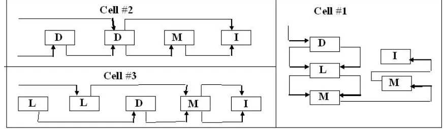
• Formal machine cells. This is the conventional GT approach in which a group of

2. Literature review

Figure 2.1 The machines in a formal machine cell are located in close proximity to minimize Part handling, throughput time, setup, and work – in progress.

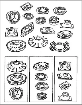
2.4 Product Application

Figure 2.2 The database of existing parts is then scanned to find items with identical or similar codes.

2.5 Summary

3. Basic principle of GT

3. Basic Principle of Group Technology

3.1 Introduction

Group technology (GT) is a manufacturing philosophy that identifies and exploits the underlying sameness of parts and manufacturing processes. In batch – type manufacturing for multi – products and small – lot – sized production, conventionally each part is treated as unique from design through manufacture. However, by grouping similar parts into part families based on either their design or processes, it is possible to increase the productivity through more effective design rationalization and data retrieval, manufacturing standardization and rationalization.

3.2 Part families

three methods are: (1) visual inspection, (2) parts classification and coding, and (3) production flow analysis.

3. Basic principle of GT

Figure 3.2 Parts having similar design features such as geometric shape, size, materials and etc.

3.3 Visual inspection (Intuitive grouping)

Figure 3.3 Intuitive grouping or visual inspection for simple part/process mixes.

3.4 Parts classification and coding

3. Basic principle of GT

the correlation is less than perfect. Accordingly, classification and coding systems are devised to include both a part’s design attributes and its manufacturing attributes. Reasons for using a coding scheme include:

• Design retrieval. A designer faced with the task of developing a new part

can use a design retrieval system to determine if a similar part already exists. A simple change in an existing part would take much less time designing a whole new part from scratch.

• Automated process planning. The part code for a new part can be used to

search for process plans for existing parts with identical or similar codes. • Machine cell design. The part codes can used to design machine cells

capable of producing all members of a particular part family, using the composite part concept.

coding system design, initial coding and family development. It is not a task for the novice.

The classification and coding procedure may be carried out on the entire list of active parts produced by the firm, or some sort of sampling procedure may be used to establish part families. For examples, parts produced in the shop during a certain time period could be examined to identify part family categories. The trouble with any sampling procedure is the risk that the sample may be unrepresentative of the population.

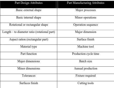
3.4.1 Features of parts classification and coding systems

The principal functional areas that utilize a parts classification and coding system are design and manufacturing. Accordingly, parts classification systems fall into one of the three categories:

1. systems based on part design attributes

2. systems based on part manufacturing attributes

3. systems based on both design and manufacturing attributes

3. Basic principle of GT

Part Design Attributes Part Manufacturing Attributes

Basic external shape Major processes

Basic internal shape Minor operations

Rotational or rectangular shape Operation sequence

Length – to diameter ratio (rotational part) Major dimension Aspect ration (rectangular part) Surface finish

Material type Machine tool

Part function Production cycle time

Major dimensions Batch size

Minor dimensions Annual production

Tolerances Fixture required

Surfaces finish Cutting tools

Table 3.1 Design and Manufacturing Attributes typically included in a Group Technology classification and coding system.

In terms of the meaning of the symbols in the code, there are three structures used in classification and coding systems:

1. Hierarchical structure, also known as a monocode, in which the interpretation of each successive symbol depends on the value of the preceding symbol.

Example:

2 == Rotational parts.

Within these groups, we can further classify by feature: presence of hole(s). 0 == No holes

1 == Has holes

Figure 3.4 Hierarchical structure.

Advantages of monocodes:

1. With just a few digits, a very large amount of information can be stored 2. The hierarchical structure allows parts of the code to be used for information at different levels of abstraction.

Disadvantages:

1. Impossible to get a good hierarchical structure for most features/groups 2. Different sub-groups may have different levels of sub-sub-groups, thereby leading to blank codes in some positions.

3. Basic principle of GT

Advantages:

1. Easy to formulate Disadvantages:

1. Less information is stored per digit; therefore to get a meaningful comparison of, say, shape, very long codes will be required.

2. Comparison of coded parts (to check for similarity) requires more work.

3. mixed – mode structure, In this case, the code for a part is a mixture of polycodes and monocodes. Such coding methods use monocodes where they can, and use polycodes for the other digits -- in such a way as to obtain a code structure that captures the essential information about a part shape. This is the most commonly used method of coding and classification.

Figure 3.5 Mixed – mode structure.

classification and coding systems for group technology applications is an important and complex task. Although many systems are available, each company

SYSTEM ORGANIZATION & COUNTRY

OPITZ Aachen Tech. Univ. (Germany)

OPITZ’s SHEET METAL Aachen Tech. Univ. (Germany)

STUTTGART Univ. of Stuttgart (Germany)

PITTLER Pittler Mach. Tool Co. (Germany)

GILDEMEISTER Gildemiser Co. (Germany)

ZAFO (Germany)

SPIES (Germany)

PUSCHMAN (Germany)

DDR DDR Standard (Germany)

WALTER (Germany)

AUSERSWALD (Germany)

PERA Prod. Engr. Res. Assn. (U.K)

SALFORD (U.K)

KK – 1 (Japan)

KK – 2 (Japan)

KK – 3 (Japan)

TOSHIBA Toshiba Machine Co., Ltd (Japan)

BUCCS Boeing Co., (U.S.A)

ASSEMBLY PART CODE Univ. of Massachusetts

HOLE CODE Purdue Univ. (U.S.A)

MICLASS TNO (Holland & U.S.A)

3. Basic principle of GT

should search for or develop a system suited to its needs and requirements. One of the essential requirements of a well – designed classification and coding system for group technology applications is to group part families as needed, based on specified parameters and should be capable of effective data retrieval for various functions as required.

Other types of classification and coding systems for general purposes have been developed and are used as libraries, museums, office supplies, commodities, insurance, credit cards and etc. One of the important factors in selecting a classification and coding system is to maintain a balance between the amount of information needed and the number of digit columns required to provide this information.

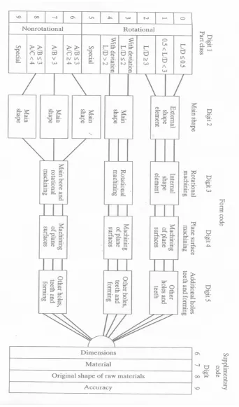
3.4.2 Opitz Classification System

This system was developed by H.Opitz of the University of Aachen in Germany. It represents one of the pioneering efforts in group technology and is probably the best known, if not the most frequently used, of the parts classification and coding systems. It is intended for mechanical parts. The Opitz coding sheme uses the following digit sequence:

12345 6789 ABCD

3. Basic principle of GT

3.3 Production Flow Analysis

This is an approach to part family identification and machine cell formation that was pioneered by J. Burbidge. Production Flow Analysis (PFA) is a method for identifying part families and associated machine groupings that uses the information contained on production route sheets rather than on part drawings. Workparts with identical or similar routings are classified into part families. These families can then be used to form logical machine cells in a group technology layout. Since PFA uses manufacturing data rather design data to identify part families, it can overcome two possible anomalies that ocuur in parts classification and coding. First, parts whose basic geometries are quite different may nevertheless require similar or even identical process routings. Second, parts whose geometries are quite similar may nevertheless require process routings that are quite different.

3. Basic principle of GT

1. Data collection

The minimum data needed in the analysis are part number and operation sequence, which is contained in shop documents called route sheets or operation sheets or some similar name. Each operation is usually associated with a particular machine, so determining the operation sequence also determines the machine sequence. Additional data, such as lot size, time standards, annual demand might be useful for designing machine cells of the required capacity.

2. Sortation of routing processes

Operation or Machine Code

Cut off 01

Lathe 02

Turret lathe 03

Mill 04

Drill: manual 05

NC drill 06

Grind 07

Table 3.3 Possible code numbers indicating operation and/or machines for sortation in PFA.

3. PFA chart

3. Basic principle of GT

A B C D E F G H I Parts

Machines

1 1 1

1 1

1 1 1

1 1

1 1

1 1

1 1 1

1 2 3 4 5 6 7

Table 3.4 PFA chart, also know as Part – Machine Incidence Matrix.

4. Cluster analysis

conventional process layout. A systematic technique called Direct Clustering Technique

4. Clustering technique & Arranging machines in GT cells

4

Clustering technique & arranging machines in GT cells

4.1 Introduction

In general, GT layout planning includes three kinds of problem to be solved, (1) machine

group (GT cell) formation; (2) the layout problem of machine groups determined; and (3)

the layout problem of individual machines for each machine group. A mathematical

layout model that covers all three layout problems for group technology has not yet been

developed. Among the three problems of GT layout planning, the problem of formation

machine groups is considered most important by many researchers. For this thesis, only

two problems area will be considered, which is (1) grouping parts and machines into

families, and (2) arranging machines in a GT cell.

Basically, the problem of machine grouping is defined as follows: Given the machine –

part matrix showing which machines are required to produce each part, find groups of

machines and families of parts in such a way that each part in a family can be fully

processed in a group of machines (that is, a GT cell). A most primitive method to solve

this problem is to rearrange rows and column of the matrix on trial and error until a good

4.2 Grouping Parts and Machines by Rank Order Clustering

Rank order clustering technique, first proposed by King, is specifically applicable in

production flow analysis. It is an efficient and easy – to – use algorithm for grouping

machines into cells. In a starting part – machine incidence matrix that might be compiled

to document the part routings in a machine shop, the occupied locations in the matrix are

organized in a seemingly random fashion. Rank order clustering works by reducing the

part – machine incidence matrix to a set of diagonalized blocks that represent part

families and associated machine groups. Starting with the initial part – machine incidence

matrix, the algorithm consists of the following steps:

1. In each row of the matrix, read the series of 1’s and 0’s (blank entries =

0’s) from left to right as a binary number. Rank the rows in order of

decreasing value. In case of a tie, rank the rows in the same order as they

appear in the current matrix.

2. Numbering from top to bottom, is the current order of rows the same as

the rank order determined in the previous step? If yes, go to step 7. If no,

go to the following step.

3. Reorder the rows in the part – machine incidence matrix by listing them in

4. Clustering technique & Arranging machines in GT cells

4. In each column of the matrix, read the series of 1’s and 0’s (blank entries

= 0’s) from top to bottom as a binary number. Rank the columns in order

of decreasing value. In case of a tie, rank the columns in the same order as

they appear in the current matrix.

5. Numbering from left to right, is the current order of columns the same as

the rank order determined in the previous step? If yes, go to step 7. If no,

go to following step.

6. Reorder the columns in the part – machine incidence matrix by listing

them in decreasing rank order, starting with the left column. Go to step 1.

7. Stop.

Figures 4.1 to Figure 4.5 show how this algorithm works,

Figure 4.1 First iteration in the Rank Order Clustering.

4. Clustering technique & Arranging machines in GT cells

Figure 4.3 Third iteration in the Rank Order Clustering.

Figure 4.5 A part – machine groupings in the Rank Order Clustering.

4.3 Direct Clustering Algorithm

A problem with the Rank order clustering algorithm is that computation of weights can

become problematic when the number of parts is large. For instance, if a shop has data

for 2000 parts, then the weigh factor for the right most columns will be 2**2000, which

is too large to compute directly. To avoid this problem, King and Nakornchai proposed

the direct clustering algorithm, which is given as:

Step1. Calculate the weight of each row.

Step2. Sort rows in descending order.

Step3. Calculate the weight of each column.

4. Clustering technique & Arranging machines in GT cells

Step5. Move all columns to the right while maintaining the order of the previous

rows.

Step6. Move all rows to the top, maintaining the order of the previous columns.

Step7. If current matrix same as previous matrix, stop; else go to step 5.

Figure 4.6 to Figure 4.11show how this algorithm works.

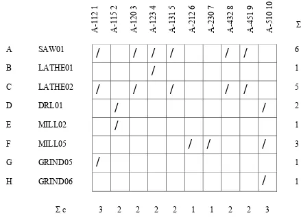
Σ r A-112 1 A-115 2 A-120 3 A-123 4 A-131 5 A-212 6 A-230 7 A-432 8 A-451 9 A-510 10

SAW01 LATHE01 LATHE02 DRL01 MILL02 MILL05 GRIND05 GRIND06 6 1 5 2 1 3 1 1

/

/

/

/

/

/

/

/

/

/

/

/

/

/

/

/

/

/

/

/

Σ c 3 2 2 2 2 1 1 2 2 3

6 7 2 3 4 5 8 9 1 10

/

/

/

/

/

/

/

/

/

/

/

/

/

/

/

/

/

/

/

/

Σ r

6 5 3 2 1 1 1 1 A C F D B E G H

Σ c 1 1 2 2 2 2 2 2 3 3

Figure 4.7 (above) & Figure 4.8 (below) 2nd & 3rd iteration.

6 7 2 10 3 4 5 8 9 1

/

/

/

/

/

/

/

/

/

/

/

/

/

/

/

/

/

/

/

/

Σ r

6 5 3 2 1 1 1 1 A C F D B E G H

4. Clustering technique & Arranging machines in GT cells

2 6 7 10 4 3 5 8 9 1

/

/

/

/

/

/

/

/

/

/

/

/

/

/

/

/

/

/

/

/

Σ r

6 5 3 2 1 1 1 1 A C F D B E G H

Σ c 1 1 2 2 2 2 2 2 3 3

Figure 4.9 (above) & Figure 4.10 (below) 3rd &4th iteration.

2 6 7 10 4 3 5 8 9 1

/

/

/

/

/

/

/

/

/

/

/

/

/

/

/

/

/

/

/

/

Σ r

6 5 3 2 1 1 1 1 A C G F D B E H

2 6 7 10 4 3 5 8 9 1

/

/

/

/

/

/

/

/

/

/

/

/

/

/

/

/

/

/

/

/

Σ r

6 5 3 2 1 1 1 1 A C G B F D H E

Σ c 1 1 2 2 2 2 2 2 3 3

Figure 4.11 Two groups of families have been formed.

4.4 Arranging Machines in a GT Cell

After part-machine groupings have been identified by direct clustering technique, the

next problem is to organize the machines into the most logical arrangement. A simple yet

effective method suggested by Hollier, use data contained in From – To charts to arrange

the machines in an order that maximizes the proportion of in-sequence moves within the

4. Clustering technique & Arranging machines in GT cells

1. Develop the From - To chart from the routing data. The data contained in the

chart indicates numbers of part moves between the machines in the cell.

2. Determine the “From” and “To” sums for each machine. This is accomplished

by summing all of the “From” trips and “To” trips for each machine. The “From”

sum for a machine is determined by adding the entries in the corresponding row,

and the “To” sum is found by adding the entries in the corresponding column.

3. Assign machines to the cell based on minimum “From” or “To” sums. The

machine having the smallest sum is selected. If the minimum values is a “To”

sum, then the machine is placed at the beginning of the sequence. If the minimum

value is a “From” sum, then the machine is placed at the end of the sequence.

4. Reformat the From – To chart. After each machine has been selected, restructure

the From – To chart by eliminating the row and column corresponding to the

selected machine and recalculated the “From” and “To” sums. Repeat steps 3 and

4 until all machines have been assigned. An example shown below:

From / To 1 2 3 4

1 0 5 0 25

2 30 0 0 15

3 10 40 0 0

4 10 0 0 0

From / To 1 2 3 4 “From

sums”

1 0 5 0 25 30

2 30 0 0 15 45

3 10 40 0 0 50

4 10 0 0 0 10

“To” sums 50 45 0 40 135

Table 4.1a From and To sums: First Iteration.

From / To 1 2 4 “From

sums”

1 0 5 25 30

2 30 0 15 45

4 10 0 0 10

“To” sums 40 5 40 135

Table 4.1b From and To sums: Second Iteration with Machine 3 removed.

From / To 1 4 “From

sums”

1 0 25 25

4 10 0 10

“To” sums 10 25

5. Plant layout

5. Plant Layout

Generally, layouts can be classed into three major categories, process layout, product layout and fixed position, although several offshoots are possible.

5.1 The Job Shop (or Process) Layout

The process type layout groups (as shown in Figure 5.1) similar machines together. Such a layout makes sense if jobs are routed all over the place, there is no clear dominant flow to the process, and tooling and fixturing need to share. For example, if the process sheets calls next for grinding, in process type layout, it is clear where the job is to be routed. The job can then enter the queue of work for the next available grinder in the group. If, on the other hand, grinding machines were scattered throughout the factory, there would be chaos. The job of production control and materials handling would be difficult; priorities and machine availabilities would be very tough to track and to execute well.

Figure 5.1 Process type layout.

5.2 The Line Flow (Product – Specific) Layout

5. Plant layout

There are a variety of line flow or product specific layouts. At one extreme are the continuous flow process layouts, with their very high capital intensity. For these processes, it is very true that the process is the layout and the layout is the process. Changing one mean changing the other and any changes involve tremendous expense, and, for that reason, are accomplished only occasionally.

At the other extreme are worker – paced line flow processes that do not involve much plant and equipment. Rather, they are more labor and materials intensive. These processes are very flexible; they can be rebalanced, turned, lengthened, chopped up, and so on with comparative ease. Lying in between the extremes are machine – paced lines that are more flexible than the continuous flow process but not as flexible as worker – paced lines.

Figure 5.2 Product – specific layout.

5.3 Fixed position layout

5. Plant layout

problematic in fixed position layouts. Inspectors often have to roam, and that may waste operators’ time as they wait on inspection. Moreover, one does not have the luxury of evaluating the process capabilities of just one machine or one station along the line; there many stations to evaluate, as many stations as there are stalls filled with worker – in process.

5.4 Group Technology Layout

In essence, group technology (or Cell manufacturing), as shown in Figure 5.3, is the conversion of a job shop layout into a line flow layout. Instead of grouping similar machines together, group technology may call for grouping dissimilar machines together into a line flow process all its own. In the new arrangement, a part can travel from one machine to another without waiting between operations, as would be customary in the job shop. Work – in – process queues of material are thus reduced; individual parts move more quickly through the process.

line’s schedule of production. With a U – line, parts fabrication that traditionally was accomplished elsewhere in the factory and in big batches is done

Figure 5.3 A group technology layout.

5. Plant layout

5.5 Orford Refrigeration Machine Shop Layouts.

5. Plant layout

6. Inventory Control

6.1 Introduction

It is not too far off the mark to visualize the problem of managing either raw materials inventory or finished goods inventory as one of managing piles of “stuffs” that process itself or consumes in the marketplace draw down. The objective of good inventory (see Figure 6.1) management is to offer good service to either the process or the market at reasonably low cost. This objective, in turn, means deciding how many items should be in each pile, when orders to replenish the piles ought to be placed, and how much each of those orders should contain. Managing such inventory stocks essentially means deciding the pile size, order time and order size.

6.2 The Periodic Reorder System

6. Inventory control

delivery lead time. The amount ordered each time was the difference between the desired level and the actual amount on – hand at the time the order was placed. Thus, it equals the actual demand during the previous period. Note that during the time period 2, the actual inventory dipped into the safety stock because of unforeseen demand.

Point of order receipt

Point at which order is placed

Lead time for delivery

A B C D

Safety stock Quantity of inventory Desired level of Inventory

Slope of line = rate of demand

0 1 2 3 4 Time periods

Figure 6.2. The periodic reorder system.

6.3 The Reorder Point System

6. Inventory control

Replenishment lead line Slope of line = rate of demand

Lead time delivery Consumption during replenishment lead-time Quantity of inventory Reorder point Safety stock level

Order #1 Order #2 Order #3 Order #4

Time

Figure 6.3. The reorder point system.

6.4 Economic Order Quantity

the Reorder Point inventory system inherent in the EOQ model. An order quantity, Q is received and is used up over time at a constant rate. When the inventory level decreases to the reorder point, a new order is placed; a period of time, referred to as lead time, is required for delivery. The order is received all at once just at the moment when demand depletes the entire stock of inventory – the inventory level reaches 0 – so there will be no shortages. This cycle is repeated continuously for the same order quantity, reorder point, and lead time.

Annual cost ($)

Total cost

Slope = 0

Minimum total cost

Carrying cost

Ordering cost

Optimal order Order

quantity

Figure 6.4 The EOQ cost model.

6. Inventory control

exactly with the point with where the carrying cost curve intersects the ordering cost curve. This can be express by the following equation:

c o opt

C

Q

C

Q

=

2

The total minimum cost is determined by substituting the value for the optimal order

size,

Q

2

min

opt c

opt

o

C

Q

Q

D

C

TC

=

+

6.5 Orford Refrigeration Inventory Systems

7. Results and discussion

A few problems have been encounter when conducting Production Flow Analysis for Orford Refrigeration. And these problems have directly affected not only the aims and objectives of this project, but also the ongoing progress of the research. The problems mentions are as follows:

1. Incomplete data needed for analysis.

7. Results and discussions

2. Parts produced are considered too simple.

Most of the parts manufactured by Orford Refrigeration are relatively simple in design and manufacturing processes. Although many types of parts have been study in order to form a part families, but it was unable to determine the parts

Figure 7.1 Folding machine.

Figure 7.2 Another type of machine used for folding process.

7. Results and discussions

Basically, the overall process to manufacture parts from sheet metal is either through the punching process and folding process or even sometime certain parts only went through one of the process only. Some of the machines (shown in Figure 8.0) can even perform all the complicated punching operation alone which further simplified the processes.

Figure 7.4 Outer back – upper.

Figure 7.6 Castor plate – front.

Figure 7.7 TOM – type A.

7. Results and discussions

Figure 7.9 Global 2.0, a very high capacity punching machine.

References

Alan Muhlemann, John Oakland and Keith Lockyer, 1992, Production and Operation Management, Sixth Edition, Pitman Publishing.

Burbidge, J L, 1977, A manual method of production flow analysis, The Production Engineer, volume 56, 1977, p.34 – 38.

Burbidge, J L, 1977, Production flow analysis, The Production Engineer, volume 41, 1977, p.742 – 752.

C.D.J. Waters, 1992, Inventory Control and Management, John Wiley and Sons Inc, Canada, p.48 - 71

Inyong Ham, Katsundo Hitomi and Teruhiko Yoshida, 1985, Group Technology – Applacations to Production Management, Klumar Nijhoff Publishing.

John W. Toomey, 2000, Inventory Management – Principles , Concepts and Techniques,

References

King, J. R., 1980, Machine – component grouping in production flow analysis: an approach using a rank order clustering algorithm, International journal of production research, volume 18, Number 2, 1980, p.213 – 232.

Mikell P. Groover, 2001, Automation, Production Systems, and Computed – Integrated Manufacturing, Second Edition, Prentice Hall Inc, New Jersey, United States of America.

Richard J. Tersine, 1994, Principle of Inventory and Materials Management, 4th Edition, Prentice Hall, p.180 – 193.

Robert S. Russell, Bernard W. Taylor III, 2000, Operations Management, 2nd Edition, Prentice Hall, Inc., United States of America

Scott M. Shafer and Jack R. Meredith, 1990, A comparison of selected manufacturing cell formation techniques, International journal of production research, volume 28, Number 4, 1990, p.661 – 673.