Smoothed Particle Hydrodynamics

(1)

Rochester Institute of Technology

RIT Scholar Works

Theses

7-26-2018

Smoothed Particle Hydrodynamics

Tanmayee Gupte

tmg9722@rit.edu

Follow this and additional works at:https://scholarworks.rit.edu/theses

This Thesis is brought to you for free and open access by RIT Scholar Works. It has been accepted for inclusion in Theses by an authorized administrator of RIT Scholar Works. For more information, please contactritscholarworks@rit.edu.

Recommended Citation

(2)

R.I.T

SMOOTHED PARTICLE

HYDRODYNAMICS

Tanmayee Gupte

A Thesis Submitted in Partial Fulfillment of the

Requirements for the Degree of Master of Science in

Astrophysical Sciences & Technology

School of Physics and Astronomy

College of Science

Rochester Institute of Technology

Rochester, NY

(3)

ASTROPHYSICAL SCIENCES AND TECHNOLOGY

COLLEGE OF SCIENCE

ROCHESTER INSTITUTE OF TECHNOLOGY

ROCHESTER, NEW YORK

CERTIFICATE OF APPROVAL

M.S. DEGREE THESIS

The M.S Degree Thesis of Tanmayee Gupte has been

examined and approved by the thesis committee as

satisfactory for the thesis requirement for the M.S.

degree in Astrophysical Sciences and Technology.

Dr. Joshua Faber, Thesis Advisor

Dr. Jason Nordhaus, Committee Member

Dr. Nathaniel Barlow, Committee Member

Date

(4)

Abstract

Smoothed particle hydrodynamics (SPH) is a meshfree particle method based on a

Lagrangian formulation, which has been widely applied to different areas in astrophysics

involving complicated fluid dynamical processes. For the first part of this project we have

expanded an existing smoothed particle hydrodynamic code (StarCrash). We have added

different time integration methods and used them to study the code’s overall ability to

conserve energy. In the second part we have evaluated the StarCrash code’s ability to use

different numerical treatments to perform shock tube simulations via Sod’s shock tube

test. We have used different evolution schemes involving either the energy or the entropy

of the system, along with different artificial viscosity formulations, and compared the

results from the numerical simulations with the analytical solution.

(5)

List of Figures

2.1 Difference between Eulerian and Lagrangian methods . . . 4

2.2 Sketch of the interaction of a particle a, with its neighboring particles.

Kernels having a finite support (shown by shaded region) are used to

prevent computationally expensive interaction of each particle with all the

other particles. The support size of a particle a is set as a multiple, Qhi,

of its smoothing length,hi. Often,Q = 2 is used, specifically that of cubic

spline (Rosswog, 2015). . . 8

4.1 Comparison between the time evolution techniques: Leap frog, Euler, RK2

and RK4 where h is the same . . . 22

4.2 Comparison between the time evolution techniques: Leap frog, RK2 and

RK4 . . . 22

4.3 Plots of position of the binaries in the xy plane at t = 3,6,9,12,15,18,21,24,30,

dynamical time used for comparing different time integration methods. For

these figure we have integrated the system using Leap Frog integration

method . . . 24

5.1 Schematic diagram of Shock tube problem . . . 26

5.2 Exact solution of Sod’s Shock tube test, Density versus position at t = 0.2. 28

5.3 Exact solution of Sod’s Shock tube test, Velocity versus position at t = 0.2. 28

5.4 Exact solution of Sod’s Shock tube test, Pressure versus position at t = 0.2. 28

7.1 Plots of density, velocity and pressure versus position for entropy evolution

technique without AV at t=0.2 . . . 35

(9)

7.2 Plots of density, velocity and pressure versus position for energy evolution

technique without AV at t=0.2 . . . 35

7.3 Plots of density, velocity and pressure versus position for entropy evolution

technique with AV at t=0.18 . . . 36

technique with AV using standard SPH equations at t=0.18 . . . 37

technique with AV using SPH methods inspired from Riemann solvers at

t=0.18 . . . 38

(10)

Chapter 1

Introduction

Many astrophysical systems have been shaped by complicated fluid dynamical processes,

e.g., hot gas in galaxy clusters, the formation of stars, and the internal structure of

galax-ies. They involve complex physical processes such as magnetic fields, nuclear burning and

usually lack symmetry. For these systems, an analytical treatment is not possible and

one must use a numerical approach.

A good numerical method will conserve various physical quantities like energy and angular

momentum. Along with it, fixed boundary conditions are usually absent, leading to

dynamically changing flow geometries. Therefore, high spatial adaptivity is a must for

their computer simulations. Hence a good choice of numerical method fulfilling the earlier

requirements is needed.

Smoothed Particle Hydrodynamics (SPH) is a particle-based Lagrangian Method

in-vented by (Lucy, 1977) to simulate nonaxisymmetric phenomena in astrophysics. It

is a method used for calculations involving self-gravitating fluids moving freely in 3D.

It has been used to study many astrophysical systems, including large scale structure,

galaxy formation, tidal disruption of stars by massive black holes and also coalescing

com-pact binaries. Coalescing comcom-pact binaries are considered as the most promising sources

of Gravitational Waves for detection from laser interferometers (LIGO, VIRGO, GEO,

TAMA). The first gravitational wave detection (B.P. Abbott et al., 2016), provided a

major new confirmation of Einstein’s theory of general relativity and the first direct proof

of existence of black holes. Compact binaries could consist of binaries of neutron stars

(11)

2 Chapter 1. Introduction

(NS) and black holes (BH), for example NS-NS, BH-NS or BH-BH. The merger of a

neutron star binary has recently been detected and is considered one of the most

impor-tant detections of Gravitational Waves (GW) as it was followed by an electromagnetic

counterpart. During the last stages of the merger of the NS, the binary begins a

transi-tion towards a rapid plunge inward, eventually leading to a merger. After passing this

point, semi-analytical methods cannot be used to describe the dynamical evolution as it

becomes too complicated due to the changing geometries and rapidly evolving metric and

hydrodynamic configuraton. Numerical simulations have been used to model coalescing

binary neutron star mergers and study the corresponding GW emission using SPH, e.g.,

the work of (Faber et al., 2004) and (Rasio and Shapiro, 1992). Other compact binaries

may also merge in ways that introduce important hydrodynamical effects with observable

consequences. Binary black holes can have mini accretion disks around them. Previous

study shows the exchange of gas between the two disks and development of spiral shocks

within the mini-disks when the binary BH separation is in the relativistic regime (Bowen

et al., 2017). SPH can also be used to study the hydrodynamics of the mini-disk.

One of the most intriguing phenomena in astrophysics is the gravitational recoil that

occurs as an after-effect of a merger of a system of binary black holes. It is caused by

asymmetric emission of gravitational radiation, causing a net overall momentum in the

remnant black hole and giving it a ‘kick’. It is possible to model the recoil using numerical

simulations which are supported by observational evidence. SPH has been used to study

recoiling black holes in presence of an accretion disk and has been applied to model the

behavior of a hydrodynamical accretion disk around a black hole binary just after the

merger (Ponce, 2011) and the kick delivered to the black hole on the evolution of the disk.

SPH could also be used for modeling the ejecta from a more complex system of binary

black holes orbiting in the presence of a disk, for example the blazar OJ287 (Valtonen

et al., 1999). Such a system is assumed to consist of a large supermassive black hole

viewed directly down the jet axis. Since we see only the jet and not the surrounding disk

of the blazar, SPH can be used to numerically model the blazar and study its properties.

The primary aim of this project is to understand the working of the SPH code StarCrash

(12)

3

astrophysical systems (for example compact objects like neutron stars and black holes).

The following section summarizes the theoretical development of Smoothed Particle

Hy-drodynamics followed by a brief description of the SPH code (StarCrash). Section 3 will

describe the implementation of a shock tube, which is used as a test for the validation of

the different artificial viscosity schemes added into the SPH code. Different time-stepping

methods have been added of various orders of accuracy to the code. The various methods

are discussed in section 4. Section 5 gives a brief discussion on the shock tube problem in

1D. Section 6 includes the various artificial viscosity techniques implemented in the SPH

code. Result and analysis of the schemes mention in section 6 are presented in section 7.

The last section will summarize the conclusions drawn from the analysis carried out and

(13)

Chapter 2

2.1

Difference between Eulerian and Lagrangian

meth-ods

Smoothed Particle Hydrodynamics (SPH) was invented to simulate nonaxisymmetric

phenomena in astrophysics (Lucy, 1977) and (Gingold and Monaghan, 1977). It is

a pure Lagrangian based method i.e. a particle based method, in contrast to Eulerian

methods which are grid based methods. The main difference between the two methods

is related to the derivatives. In the Eulerian picture derivatives are calculated at a fixed

point in the space, on the other hand in the Lagrangian description they are calculated

[image:13.612.182.406.544.661.2]

in a coordinate system attached to a moving fluid element.

Figure 2.1: Difference between Eulerian and Lagrangian methods

(14)

2.2. Advantages and disadvantages of smoothed particle hydrodynamics5

2.2

Advantages and disadvantages of smoothed

par-ticle hydrodynamics

Advantages

• SPH imposes no arbitrary finite boundary on the numerical simulation and

there-fore matter is not lost or forced back into the simulation at domain boundaries,

inherently conserving the mass of the system.

• Large voids and highly distorted flows occur during impacts or mass transfer in

gas dynamics. As SPH follows particles, computational time and memory is not

wasted by keeping track of large number of empty cells as in Eulerian scheme (Benz

et al., 1990). Hence SPH offers higher computational efficiency than grid-based

calculations.

• The fluid evolution history is intrinsically simple to trace due to the particle-like

nature. In grid based codes, one would require including tracer particles to follow

the flow of the fluid.

• Another advantage of SPH is accomplishment of fluid advection even for stars with

a sharply defined surface like NS as particles follow their trajectories in the flow.

Tracking of hydrodynamic ejection of matter to large distances from central dense

region is also easy with SPH.

• Particle nature makes coupling to N-body or self-gravity physics relatively

straight-forward.

Disadvantages

• In SPH one must build and constantly update neighbour lists (by linked-lists or

binary trees) in order to evaluate particle summations.

• The initial conditions can be influential on the eventual outcome and therefore one

must decide on whether to set particles on a cubic, hexagonal or random lattice

(15)

6 Chapter 2. Smoothed Particle Hydrodynamics

• Lastly in SPH resolution is limited by particle number, which is fixed at the start

of the simulation, whereas in theory a grid can be sub-divided indefinitely.

2.3

Theoretical development of SPH

2.3.1

Lagrangian hydrodynamics

As mentioned earlier SPH is a purely Lagrangian approach, where the derivatives are

calculated in a coordinate system attached to a moving fluid element. The time derivative

in the Lagrangian approach (d/dt) is related to the Eulerian derivative ∂/∂t by

d dt =

dxi dt

∂ ∂xi +

∂

∂t =~v· ∇+

∂

∂t, (2.1)

where x/,(i= 1,2 and 3) is position and~v is the velocity, when applied to the continuity equation in the Eulerian approach

∂ρ

∂t +∇ ·(ρ~v)= 0, (2.2)

using equation (2.1) for taking the derivative of ρ (density) one finds in the Lagrangian

form

dρ

dt = −ρ∇ ·~v. (2.3)

The conservation of momentum equation in the Lagrangian forms becomes

d~v dt =−

∇P

ρ + ~f. (2.4)

Equation 2.4 shows that apart from forces like magnetic fields or gravitation included in

the quantity ~f, the fluid gets accelerated by pressure P gradients. Similarly the energy

equation can be derived from the first law of thermodynamics and equation (2.3)

du dt =

P

ρ2

dρ dt =−

P

(16)

2.3. Theoretical development of SPH 7

2.3.2

The SPH kernel interpolation

In this section, the discrete form of continuous Lagrangian hydrodynamics equations

will be discussed. As mentioned earlier, in the SPH method the interpolation points

“particles” move with the local fluid and the derivatives are calculated with a kernel

approximation without finite differencing. Therefore the partial differential equations

(PDEs) of Lagrangian fluid dynamics are converted into ordinary differential equations.

In order to conserve the physical quantities by construction in the PDEs, they need to

have correct symmetries in the particle indices. The “Vanilla ice” version of SPH has

this symmetry (Rosswog, 2009).

2.3.2.1 Interpolating function values

The kernel function is a key parameter of SPH, and defines how many particle neighbours

we care about when calculating fluid properties. With the help of, kernel function we can

interpolate particle properties from the neighbouring particles. The main idea of SPH

can be explained by the kernel approximation in which a function f(~r) is approximated

by

~

fh =

Z

f(~r)W(~r−~r0,_h₎_d3_r~0, _(2.6)

whereW is called smoothing kernel andh is the smoothing length, which determines the

rate of radial decay. The functionf is integrated over all other fluid elements at positions ~

r0_{. The above integral is formulated into a summation over a set of interpolation points}

throughout the medium, (the SPH particles). It means we can estimate the function f

for some particle at~r by a weighted sum of that samef evaluated at every other particle

(17)

[image:17.612.194.391.91.253.2]

Figure 2.2: Sketch of the interaction of a particlea, with its neighboring particles. Kernels having a finite support (shown by shaded region) are used to prevent computationally expensive interaction of each particle with all the other particles. The support size of a particle a is set as a multiple, Qhi, of its smoothing length, hi. Often, Q = 2 is used,

specifically that of cubic spline (Rosswog, 2015).

In order to recover the original function the kernel should fulfill, in limit of infinitely

small smoothing region

lim

h→0 ~

fh(~r)= f(~r) and

Z

W(~r−r~0,_h₎_d3~

r0= 1, _(2.7)

The integral can be written as

~

fh(~r)=

Z

f(~r)

ρ(~r)W(~r−r~

0,_h)ρ(_r~0₎_d3~_r0, _(2.8)

which after replacing the integral by a sum over a set of interpolation points (particles)

whose masses are mj, gives

f(~r)=X

j

= mj

ρj

fjW(~r−r~0,h). (2.9)

Equation 2.9 can be used to get the density as

ρ(~r)= X

j

(18)

The density estimation (equation 2.10) given by summing up kernel weighed masses in

the neighbourhood of point~r plays a crucial role in the derivation of Lagrangian SPH

derivations. It satisfies the continuity equation and therefore conserves mass of the

system.

2.3.2.2 Approximating derivatives

The derivatives can be calculated by taking equation 2.9 and we get

∇f(~r)=X

j mj

ρj

∇W(~r−r~0,_h), _(2.11)

where the exact derivative of the approximated function is used, where Wi j is given by

∇Wi j =eî jwi j,eî j is the unit vector going from particle b to particle a, i.e. eî j =~ri j/ri j and

~ri j =~ri−~rj

2.3.2.3 The kernel function

SPH usually uses radial kernels withW(~r−r~0,_h₎= _W₍_|~_r₋_r~0_|,_h₎_{.The kernel should also be}

smoothly differentiable (at least singularly) and be an odd function and≥0 in all space.

In most SPH simulations standard cubic spline SPH kernel is used (Monaghan, 1992)

and is also used by StarCrash. In 3D the cubic spline is given as

W(q)= 1 πh3

                

1− 3₂q2+ ₄3q3 for 0≤q≤1

1

4(2−q)

3 _for ₁_<q _≤ ₂

0 for q >2,

(2.12)

where q=|~r−r~0_|/_h _{. Since this kernel only depends on the absolute value of}_|~_r₋_r~0_|_{, it is}

radial.

2.3.3

The “vanilla ice” SPH equation

2.3.3.1 Momentum equation

The following derivations of conservation of momentum and energy are derived from the

(19)

Spatially discretizing equation (2.4) gives

d~vi dt = −

1 ρi X j mj ρj

Pj∇iWi j, (2.13)

this form will solve the Euler equation but does not conserve momentum. The force on

particle a by particle b is given by

~

Fji=

mi d~vi

dt

j

= −mi ρi

mj

ρj

Pj∇iWi j, (2.14)

and the force on particle b due to particle a is

~

Fi j =

mj d~vj

dt

i =

−mj ρj

mi

ρi

Pi∇jWji = mi

ρi mj

ρj

Pi∇iWi j. (2.15)

As Pi ,Pj, by construction Newton’s third law is not fulfilled (Every action has an equal

and opposite reaction), and total momentum is also not conserved. However if we start

by the following equation instead of equation (2.4), momentum gets conserved

∇ _P

ρ

= ∇_ρP −P∇ρ

ρ2, (2.16)

if one solves for ∇P/ρ and applies the gradient formula, equation (2.11), the momentum

equation gets converted to

d~vi dt = −

X

j mj

_P

i

ρi2 + Pj

ρj2

∇iWi j. (2.17)

As the part of the equation having the pressure term is symmetric and ∇iWi j = −∇jWji,

the forces are equal and opposite. By construction the total momentum and angular

momentum is conserved. Thus we have a system of ODEs which have been used to

(20)

2.3.3.2 Energy equation

Spatially discretizing the energy one obtains,

dui dt =

Pi

ρi2 dρi

dt = Pi

ρi2 d dt

X

j

mjWi j

= Pi

ρi2

X

j

mj~vi j· ∇iWi j. (2.18)

Equation (2.10), (2.17) and (2.18) are the complete set of SPH equations. An alternate

form of the energy equation can be derived on using the “thermokinetic” energy eˆi =

ui + 1₂vi2 instead of specific internal energy ui. This equation will allow a smoother

transition to the relativistic equations. The following evolution equation

deˆ

dt = −

1

ρ∇ ·(P~v), (2.19)

can be converted to

deˆ

dt = − P

ρ2∇ ·(ρ~v)−~v· ∇ P

ρ

, (2.20)

On applying equation (2.11) to equation (2.20) this becomes

deˆi dt =

X

j mj

P_i~v_j ρi2

+ Pj~vi

ρj2

· ∇iWi j. (2.21)

The above form of energy equation is useful as it is similar to the relativistic equation.

If one is dealing with artificial viscosity (AV) additional terms need to be added to the

equation (2.21). Artificial viscosity is used for handling shocks. The equation is given by

deˆi dt =

X

j mj

P

i~vj

ρi2

+ Pj~vi

ρj2 + Πi j

(vi+vj)

2

· ∇iWi j, (2.22)

where Πi j is the artificial viscosity (AV). See chapter 6 for more on AV formalism and

tests.

2.3.4

Different evolution techniques

The system is evolved using energy if one uses equation (2.22). The advantage of using

(21)

• conservation of energy

• allowing shock capturing technique if one adds artificial viscosity to the equation.

Another method of evolving the system is by using entropy change. The change in

entropy is given as

dAi dt =

Γ−1 2ρΓ−1

i

X

j

mjΠi j(~vi−v~j)· ∇Wi j (2.23)

where Ai is defined in the polytropic equation of state Pi = AiρiΓ and Γ is the ratio of

specific heats. The given evolution scheme (equation 2.23) is used in the code StarCrash.

The advantage of using entropy change techniques are

• pressure is always numerically positive

• the second law of thermodynamics is automatically satisfied.

Both the schemes imply conservation of total momentum and total energy (Rasio, 1991)

(22)

Chapter 3

code - StarCrash

In this project we have used the SPH code StarCrash, which is a parallel based

hy-drodynamics code originally developed by Rasio and Shapiro to study merging binaries

(Rasio and Shapiro, 1992, 1994, 1995), and parallelized by Faber and Rasio for use in

post-Newtonian calculations of coalescing neutron stars (Faber and Rasio, 2000; Faber

et al., 2001; Faber and Rasio, 2002). In the following chapter, the basic equations and

features of StarCrash are briefly discussed.

3.1

Basic equations used in StarCrash

The basic formulation of the SPH equations used in the code StarCrash is summarized

in this section. The SPH density used in StarCrash is calculated using a slightly altered

formula as opposed to equation (2.10). The density of particle ‘i’ is given as

ρi =

X

j mj

W(|~ri−~rj|,hi)+W(|~ri−~rj|,hi)

2 , (3.1)

where~ri is the actual position of the particle i and W is the Kernel function. The code

uses the “gather-scatter” algorithm, i.e., for each particle-neighbor pair, it counts half of

the density contribution to the particle, and half to the neighbor. The Kernel function is

defined such that it drops to zero at a radius equal to 2 smoothing lengths. The Kernel

(23)

14 Chapter 3. Smoothed Particle Hydrodynamics code - StarCrash

function is given by equation (2.12). The pressure at~ri is calculated by

Pi = AiρiΓ, (3.2)

where Ai is the specific entropy function at ~ri. The hydrodynamical part of the force is

calculated by

~

Fihydro =−

X

j mimj

Pi

ρi2 + Pj

ρj2

+ Πi j ∇iWi j. (3.3)

This form has the advantage of being computationally convenient while at the same time

fulfilling a natural set of conservative laws.

3.1.1

Artificial Viscosity

In the code StarCrash three different kinds of artificial viscosity schemes are are

intro-duced. The user has the option of using a suitable scheme

3.1.1.1 Monaghan

For artificial viscosity a symmetrized version of the form proposed by (Monaghan, 1989)

is adopted

Πi j =

−αµi jci j+βµi j2

ρi j

, (3.4)

where ρi j = (ρi +ρj)/2 and ci j = (ci+cj)/2 (ci is the sound speed given as ci = (ΓPi/ρi)

1 2

and

µi j =

        

(v~i−v~j)·(r~i−r~j)

hi j(|~ri−r~j|2/hi j2+η2), when (~vi

−v~j)·(~ri−r~j) < 0

0, when (~vi−v~j)·(~ri−r~j)≥0,

(3.5)

with hi j = (hi + hj)/2, representing a combination of von Neuman-Richtmyer artificial

viscosity and bulk viscosity.

3.1.1.2 Hernquist and Katz

A second form of AV (Hernquist and Katz, 1989) used in the code calculates Πi j from

(24)

3.1. Basic equations used in StarCrash 15

Πi j =

         qi

ρi2 +

qj

ρj2 if (~vi−v~j)·(~ri−r~j) <0,

0, if (~vi−v~j)·(~ri−r~j)≥0,

(3.6)

where

qi =

        

αρicihi|∇ ·~ ~v|i+βρihi2|∇ ·~ ~v|2_i if (~∇ ·~v)i<0,

0, if (~∇ ·~v)i ≥0,

(3.7)

and

(∇ ·~ ~v)i =

1 ρi

X

j

mj(v~j−v~i)·~∇Wi j (3.8)

3.1.1.3 Balsara

A third form of AV technique used in StarCrash was developed by (Balsara, 1995) given

by

Πi j =

_p

i

ρi2 + pj

ρj2

(−αµi j+βµ2i j), (3.9)

where

Πi j =

        

(v~i−v~j)·(r~i−r~j)

hi j(|~ri−r~j|2)/hi j2+η2

fi+fj

2ci j if (~vi−v~j)·(~ri−r~j) <0,

0, if (~vi−v~j)·(~ri−r~j)≥ 0.

(3.10)

In this equation fi is the function defined by

fi =

|~∇ ·~v|i

|~∇ ·~v|i+|~∇ ×~v|i+η0ci/hi

, (3.11)

the factorη0 = 10−5 _{is used to avoid divergence and}

(∇ ×~ ~v)i =

1 ρi

X

j

mj(~vi−v~j)×∇~Wi j. (3.12)

3.1.2

First law of thermodynamics

There are two methods for evolving a system using SPH. As mentioned in section (2.2.3)

we can evolve the system using energy and hence conserve energy and momentum, in

(25)

16 Chapter 3. Smoothed Particle Hydrodynamics code - StarCrash

use entropy for evolving the system. The first law of thermodynamics at position ~ri is

given by

dAi dt =

Γ−1 2ρiΓ−1

X

j

mjΠi j(~vi−v~j)· ∇iWi j. (3.13)

Both the methods are used for different reasons. The advantage of using entropy

evo-lution is, that the entropy will never decreases with time. Since the kernel W(r,h) is a

monotonically decreasing function of r, the right hand side of the equation is positive as

Πi j>0when (~vi−v~j)·(~ri−r~j)<0and is zero otherwise. On the other hand the positivity

of the internal energyui is not guaranteed, when equation (2.18) is used and can lead to

large errors. However there are disadvantages in using the first law of thermodynamics

when time dependent smoothing lengths are used. It can lead to errors in conservation of

total energy. The use of time dependent smoothing lengths is necessary to ensure correct

spatial resolution throughout a calculation. As the fluid expands and contracts the local

values of hi must continually adapt so that number of neighbours NN for any particle

remains constant with time.

3.1.3

The gravity solver

The SPH method requires a very large number of particles to provide accuracy. Therefore

a direct summation method to calculate the gravitational field of the system is ruled out.

StarCrash uses a grid-based method for calculating the gravitational field of the system.

The values of source term for the Poisson equation is calculated by the definition of

density given by ρi =PjmjWi j. The gravitational potential and force for each particle is

calculated by FFT convolution. According to Newton’s Law the Gravitational Potential

is given by

φ(~r)= Z

ρ(r~0₎d

3₍~_r0₎

|~r−r~0_| =

X

i mi

|~r−~ri|

. (3.14)

The direct sum would require N2 _{operations and is computationally expensive. The}

integral can be converted in a form of convolution

φ(~r)=FFT−1×

FFT(ρ)∗FFT ₁

(26)

3.2. Number of Neighbours 17

whereFFT−1 denotes the inverse Fast Fourier Transform. In order to use the convolution

technique, the data is imported to a 3-dimensional grid.

3.1.4

Leap-frog technique

The time evolution techniques are integrated using the Leap Frog method. Please see

section (4.2) for more details.

3.1.5

Relaxation

A common problem faced by SPH codes is that the initial configuration of the system

may not be in an equilibrium and the resulting oscillations can lead to misleading results.

Therefore the SPH code StarCrash introduces a routine that relaxes the material

config-uration before computing a dynamical run. A drag term is added to the forces calculated

by standard techniques

d~v dt =~a−

~v trelax

, (3.16)

where trelax is the relaxation time that roughly corresponds to the dynamical time given

by1/√Gρ.

3.2

Number of Neighbours

The number of neighbours used for each particle is a very important in calculation of

forces. The level of numerical noise is directly related to the number of neighbours NN,

as the noise level increases on increasing NN (Rasio and Shapiro, 1992). We can obtain

a higher level of accuracy only when we increase the number of particles N as well as

NN. The NN need to increase faster than N so that the smoothing length hi decrease

(Rasio, 1991). However the spatial resolution is proportional to 1/NN1/d ind dimensions.

Therefore, for a given calculation the choice of parameter NN will have to be imposed by

(27)

Chapter 4

Numerical integration techniques

When we are simulating an astrophysical system, made of N number of particles, we

need to solve Ordinary Differential Equations (consisting of particle positions, velocity,

acceleration, entropy etc). Very rarely can these equations be solved analytically and

one must use numerical approximation using discretized methods. In this chapter we

will be discussing the different numerical methods that have been implemented in the

code StarCrash. The following numerical methods are designed to approximate

well-posed initial value problem

y0 = f(t,y), y(t0)= y0, y∈Rd, (4.1)

such that there exists a unique solutiony(t,t0,y0)that satisfies (4.1) in the interval[t0,t0+

T∗], 0<T∗ ≤ ∞. A discrete set of y-values, yn, n = 0,1.... can be constructed using

discretisation methods given by (4.1), in such a manner that y_n should be approximated

at a corresponding set of t values (tn) with spacing h called time steps. Discretization

methods are broadly classified as implicit methods and explicit methods. Briefly, an

explicit method obtains the successive values of yn+1 parametrically in terms of given or

previously computed quantities and is represented symbolically in the form

yn+1 = H(f,tn, ....tn+1−m,yn, ....yn+1−m). (4.2)

(28)

4.1. Euler’s Method 19

and an implicit methods definesyn+1 as the solution of an equation

G(f,tn, ....tn+1−m,yn, ....yn+1−m)=0. (4.3)

Given a numerical value y0 these methods take the form

yn+1= yn+h r

X

i=1 γiy

0

n,i, n=0,1... (4.4)

where

y0_n_,_i = f(tn+αih,yn+h r

X

j=1

βi jy0n,j) and αi = r

X

j=1

βi j, (4.5)

if βi j = 0 forj ≥ i, the method is explicit, otherwise the method is implicit. The main

idea behind these methods is to get a better approximations of y(tn+1) by sampling the

vector field f(t,y) at r points near the solution curve originating from (tn,yn). A better

estimate is provided of the solution curve and therefore later samples can also be chosen

more usefully. In the next sections we will introduce four different numerical methods of

different orders. The leap frog method was incorporated into the code StarCrash. For

my project we have added three more explicit methods namely Euler and Runge Kutta

methods (second and fourth order). The number of the order is defined by the error on

the order of h to that number. For example, second order method will have errors, on

the order of h to the second power.

4.1

Euler’s Method

Euler’s method is the most elementary of the first order methods used for solving ODE’s.

Euler’s method approximates the derivative in equation (4.1) by using finite difference

y0(t)≈ y(t+h)−y(t)

h , (4.6)

where the independent variable is discretized in equal increments.

(29)

20 Chapter 4. Numerical integration techniques

Approximate values of the dependent variable are given by arranging the difference

quo-tient

yn+1 =yn+h f(tn,yn) n=0,1,2.... (4.8)

Euler’s method can also be derived from equation (4.4) by using r = 1, γ₁ = 1 and β₁₁

= 0.

4.2

Leap Frog

The leap frog method is the numerical integration method that is used in the code

StarCrash. One can derive the equations of leap frog by using taylor expansion of a

function yn+1 =y(tn+h) to second order in h

y(tn+1)=y(tn)+hy0(tn)+

1 2h

2

y00(yn,tn)+O(h3), (4.9)

with

y0(tn+1/2)=y0(tn)+(h/2)y00(yn,tn), (4.10)

can be rewritten as

y(tn+1)= y(tn)+hy0(tn+h/2)+O(h)3. (4.11)

Thus the derivative y0 needs to propagate at the intervals t(n+1/2) = tn+h/2, i.e between

the integer - labelled points of the independent variabletn = t0+nhused for the variable

‘y’. One can use

y0(tn+3/2)= y0(tn+1/2)+hy00(yn+1,tn+1). (4.12) On combining equation (4.11) and (4.12) we get,

y0n+1/2 =y

0

n−1/2+hy

00

n, (4.13)

yn+1= yn+hy 0

(30)

4.3. Runge - Kutta Second order (RK2) 21

4.3

Runge - Kutta Second order (RK2)

The Euler method as given by equation (4.8), which advances the solution through an

intervalh and uses derivative information only at the beginning of the interval. Runge

-Kutta method of the second order, uses a “trial step” at the midpoint of the interval. It

uses the values at the midpoint to calculate the solution at the end of the interval. RK2

is an explicit method. Consider the ODE

dy

dt = f(y,t) (4.15)

the second order estimate for yn+1 is given by

k1 = h f(yn,tn)

k2 = h f(yn+ k1

2,tn+

h

2)

yn+1 = yn+k2 (4.16)

where h=tn+1−tn

4.4

Runge - Kutta Fourth Order (RK4)

Higher order RK methods can also similarly be built by using same technique. For

example the fourth order RK method which is also an explicit method. The numerical

solution to the equation (4.15) can be calculated as follows

k1 = h f(yn,tn)

k2 = h f(yn+ k1

2,tn+

h

2)

k3 = h f(yn+ k2

2,tn+

h

2)

k4 = h f(yn+k3,tn+h)

yn+1 = yn+ k1

6 +

k2 3 +

k3 3 +

k4

(31)

4.5

Conservation of energy

We have incorporated the different time evolution techniques in the code StarCrash to

determine which technique is the best for conserving energy. We start with a binary

equal mass star system on a hyperbolic trajectory. The units are G = M = R = 1. The

radius and mass of the stars is 1 with separation between them 4. The following figure

[image:31.612.171.426.229.395.2]

show a comparison between the four different time evolution techniques.

Figure 4.1: Comparison between the time evolution techniques: Leap frog, Euler, RK2 and RK4 where h is the same

[image:31.612.171.423.474.646.2]

(32)

4.5. Conservation of energy 23

After looking at Figure 4.1 and Figure 4.2, we can conclude that Euler is not a good time

evolution technique as compared to Leap frog, RK2 and RK4. While the other three

give comparatively similar results with regards to conservation of energy. It is possible

to get even better conservation of energy by using the proper initial conditions and/or

reducing the time steps. The following figures will show the evolution of stars which we

(33)

[image:33.612.90.490.78.187.2]

(34)

Chapter 5

Shock Tube

The Shock tube is a Riemann problem and also a computational fluid dynamics problem

that has been of interest for many reasons. Firstly it offers a framework to solve nonlinear

hyperbolic systems of partial differential equations. Secondly, as the exact analytical

solution is known, it can be used as a difficult test for numerical methods dealing with

discontinuities.

5.1

Physical description of the shock tube problem

The shock tube can be described fundamentally as follows: consider a long one

dimen-sional tube closed at both the ends and divided in half by a thin diaphragm. Each of

the two regions are filled with the same gas but different thermodynamical properties

(pressure, density and velocity). The region with highest pressure is called as thedriving

section and the region with lowest pressure is called as the working section. The gas is

initially kept at rest and when the diaphragm breaks, a high speed flow is generated in

the working section.

In the following section we will go into a more detailed analysis of the shock tube problem.

5.2

Analysis of the shock tube problem

As shown in figure (5.1) let us consider that the left part of the shock tube is the part

with the higher pressure having pressure, density and temperature as (PL, ρL,TL) and

similarly the right side of the tube having the following parameters of pressure, density

(35)

[image:35.612.112.483.73.187.2]

26 Chapter 5. Shock Tube

Figure 5.1: Schematic diagram of Shock tube problem

and temperature (PR, ρR,Tr) with PL > PR. At time t = 0, the diaphragm breaks,

generating a process which would physically try to equalize the pressure in the entire

tube. The gas in the high pressure region will expand and flow into the working section

through an expansion (or rarefaction) wave pushing the gas of this part. The rarefaction

is a continuous process and takes place in a well defined region that propagates to the

left. The compression of the low pressure gas generates a shock wave propagating to

the right. We can assume that the expanded gas is separated from the compressed

gas through a fictitious membrane called the contact discontinuity that is travelling to

the right at a constant speed. The physical functions defining the tube namely pressure,

density, velocity and temperature are discontinuous across the shock wave and the contact

discontinuity. These will be discussed in the later section.

5.3

Euler equation of gas dynamics

Let us consider a mathematical description of the shock tube problem. In order to do this

we will assume that the tube is infinitely long, neglect viscous effects and the diaphragm

is completely removed at time t = 0. Using these simplifying hypotheses the compressible

flow in the shock tube can be described by one dimensional system of PDEs (Hirsch, 1988;

LeVeque, 1992) ∂ ∂t                  ρ ρU E                  | {z } W (x,t) +_∂∂ x                  ρU

ρU2+_p

(E + p)U                  | {z }

F(W)

(36)

5.3. Euler equation of gas dynamics 27

where density is ρ and the total energy is E. The total energy is given as

E= p

γ−1+ ρ 2U

2_. _(5.2)

For an ideal gas the equation of state is given as

p= ρRT, (5.3)

where the thermodynamic properties of the gas are described by the gas constant R

divided by molecular mass andγ is the specific heat of the gas. The local speed of sound

a, Mach number M and total enthalpy H is described by

a= pγRT =

s γP

ρ, (5.4)

M = U

a, (5.5)

H = E+ p

ρ =

a2

γ−1 + 1 2U

2_. _(5.6)

If we consider the column vectors of unknowns W =(ρ, ρU,E)t the Euler system of

equa-tions can be written as

∂W

∂t +

∂

∂xF(W)= 0, (5.7)

with the initial conditions (we denote by x0 the abscissa of the diaphragm):

W(x,0)=         

(ρL, ρLUL,EL) x≤ x0

(ρR, ρRUR,ER) x≥ x0,

(5.8)

The mathematical analysis of the Euler system of PDE’s has the form

∂W

∂t +A

∂W

(37)

28 Chapter 5. Shock Tube

with the Jacobian matrix

A=                 

0 1 0

1

2(γ−3)U

2 ₍₃₋γ)_U γ₋₁

1

2(γ−1)U

3₋_{U H} _H₋_(γ₋₁₎_U2 _γ_U_.

                 (5.10)

This gives the description of the Shock tube problem in the mathematical form.

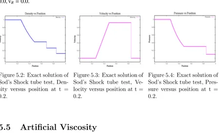
5.4

Exact solution

The following figures show the exact solution of the shock tube problem. The code used

to produce the plots has been originally written by Bruce Fryxell. The length of the tube

is 1. The conditions used for the shock tube are ρL=1,PL= 1,vL=0.0, ρR = 0.125,PR =

[image:37.612.173.427.106.171.2]

0.0,vR =0.0.

[image:37.612.75.524.318.591.2]

Figure 5.2: Exact solution of Sod’s Shock tube test, Den-sity versus position at t = 0.2.

Figure 5.3: Exact solution of Sod’s Shock tube test, Ve-locity versus position at t = 0.2.

Figure 5.4: Exact solution of Sod’s Shock tube test, Pres-sure versus position at t = 0.2.

5.5

Artificial Viscosity

When we treat the shock tube problem numerically, we see a lot of oscillations in the

numerical solution of the density/velocity variation with position (see section 7.1.1).

These oscillations can be damped by adding a supplementary term to the conservative

form of differential equations of the shock tube (5.7)

∂W

∂t +

∂

∂xF(W)−δx

2 ∂

∂x

D(x)∂W ∂x

(38)

5.5. Artificial Viscosity 29

where δx is given by 1/(M − 1) The mathematical form of this term called artificial

viscosity is inspired by the heat equation. We have discussed further on numerical AV

(39)

Chapter 6

Artificial Viscosity

6.1

Artificial Viscosity

In gas dynamics, discontinuous solutions or “shocks” can result even from perfectly

smooth initial conditions, which are nearly common in astrophysical system. Due to

the presence of physical viscosity, solutions are always smooth on length scale of gas

mean free path. On the other hand, the very steep gradients appear as discontinuous on

macroscopic scale of simulations (which is usually orders of magnitude larger).

Shocks can be dealt in two ways: (i) we can either make use of analytical solution of

a Riemann problem between two adjacent cells or particles or (ii) we can add

pseduo-microscopic terms that create entropy at shock-front, which will imitate the effect of

physical viscosity but on a scale that is numerically resolvable. The second way can be

used by adding extra “artificial” viscosity to the flow i.e. adding pressure like terms to

the fluid equations (Hernquist and Katz, 1989).

The solutions to ideal hydrodynamic equations (1.3 -1.5) can not include real

disconti-nuities with their infinite derivatives. The aim of artificial visocity (Von Neumann and

Richtmyer, 1950) is to introduce (artificial) dissipative terms into the equations in order

to give the shocks a thickness comparable to the spacing (of the grid points). Then the

corresponding differential equations can be used for the entire calculation, as if there are

no shocks in the system. The aim of artificial viscosity is not to imitate physical viscosity.

Instead it is introduced as an ad hoc method to produce on a resolvable scale, results of

(40)

6.1. Artificial Viscosity 31

small scale effects that are unresolvable.

There are a number of properties that are desirable of an AV scheme (Caramana et al.).

It must not introduce unphysical effects and should always be dissipative i.e, transfer

energy into internal energy. It should be able to distinguish uniform compression from a

shock and go to zero when compression vanishes. It should also be absent for expansion.

Lastly it must be able to conserve energy, momentum and angular momentum so that it

can be used formulated into SPH formulation.

6.1.1

Standard SPH Viscosity

An approach to incorporate artificial viscosity has been introduced by (Monaghan, 1989)

which is the most widespread form of AV scheme used in SPH. It has been discussed in

subsection (3.1.1.1) and has been used in the code StarCrash. We are discussing it in

detail over here as other forms of AV methods (that we have implemented as a part of

this project) have been developed through this scheme.

In this approach we increase the hydrodynamic pressure Pi in terms of momentum

equa-tion (2.17) by artificial contribuequa-tionΠi j

Pi

ρi2 + Pj

ρj2

!

→ Pi ρi2

+ Pj

ρj2 + Πi j

!

(6.1)

The bulk viscosity contribution toΠi j is of the formc1csh/ρ ∂v/∂xand a Taylor expansion

of the velocity field v(xi+(xj−xi)) gives

∂v

∂x

!

i

= vj−vi xj−xi

+O

(xj−xi)2

(6.2)

gives a SPH, bulk viscosity contribution

Πi j,bulk=

         -c1

~cs,i j

~ρi j for xi jvi j <0 0 otherwise

,where µi j =

~_h_{i j}_x_{i j}_v_{i j}

x2_{i j}+~h2_{i j}

(6.3)

c1 is a parameter of the order unity and cs is the sound speed. The term xi jvi j detects if

(41)

32 Chapter 6. Artificial Viscosity

The total artificial viscosity (with the von-Neumann-Richtmyer term) is given as

Πi j = Πi j,bulk+ Πi j,NR =

        

−α~ci j+βµ2_{i j}

~

ρi j for xi jvi j <0 0 otherwise

,where µi j =

~_h_{i j}_x_{i j}_v_{i j}

x2_{i j}+~h2_{i j}

(6.4)

The momentum equation after accounting for AV becomes

d~vi dt =−

X

j mj

_P

i

ρi2 + Pj

ρj2 + Πi j

∇iWi j (6.5)

and the corresponding energy equation becomes

deˆi dt =

X

j mj

P_i~v_j ρi2

+ Pj~vi

ρj2 + Πi j

(vi+vj)

2

· ∇iWi j (6.6)

This combination conserves energy, linear and angular momentum.

This is the classic AV technique and is the standard in the code StarCrash

6.2

New form of AV technique

An alternate form of was proposed by (Monaghan, 1997) which uses solutions analogous

to Riemann solvers.The main idea is that any conserved scalar variable A satisfying

X

i mi

dAi

dt = 0 (6.7)

a dissipative term of the form

_dA i dt diss = X j mj

αA,jvsig

~ρi j

(Ai−Aj)ˆei j· ∇iWi j (6.8)

needs to be added where αA,b determines the exact amount of dissipation and vsig is

the maximum signal velocity between the two particle a and b. With this form of AV

technique we get the momentum equation as

_d~_v

i dt diss= X j mj

αvsig(~vi −~vj) ˆei j

~ρi j

(42)

6.2. New form of AV technique 33

and the thermokinetic energy equations is

_d~_e_ˆ

i

dt

diss=

X

j mj

(e∗_i −e∗_j) ˆei j

~ρi j

· ∇iWi j. (6.10)

The energy along the line of sight between the two particles (Price, 2008)

e∗i =

1

2αvsig(~vi·eˆi j)

2₊_α

uvusigui (6.11)

has been used along with different signal velocities and dissipation parameters. For

non relativistic hydrodynamics, vsig which is the maximum signal velocity between two

particles is given by (Monaghan, 1997)

vsig= cs,i+cs,j−~vi j·eˆi j, (6.12)

where csk is the sound velocity of the particle k.

In the SPH code StarCrash, we have incorporated this form of AV scheme along with

the standard AV technique. The results and analysis of both the techniques is discussed

(43)

Chapter 7

Results and Analysis

7.1

Analysis

7.1.1

Shock tube without AV

In this section we will be showing the evolution of the shock tube problem without AV.

The initial conditions are ρL = 1,PL = 1,vL = 0.75, ρR = 0.125,PR = 0.0,vR = 0.0.. We

have used 1000 particles and density was calculated using summation. For this test we

used the fourth order Runge-Kutta integrator.

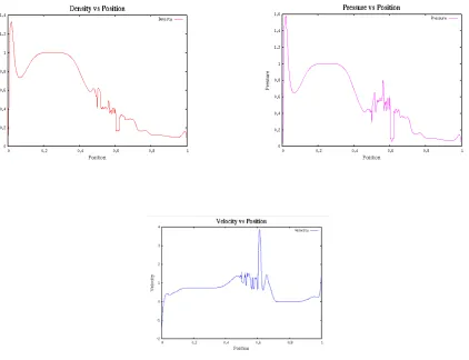
7.1.1.1 Entropy evolution technique without AV

The following figures show the evolution of the Shock tube problem (Chapter 5) using

the change in entropy (equation 2.23)

(44)

[image:44.612.214.414.71.215.2]

7.1. Analysis 35

Figure 7.1: Plots of density, velocity and pressure versus position for entropy evolution technique without AV at t=0.2

7.1.1.2 Energy evolution technique without AV

the change in energy (equation 2.22)

[image:44.612.100.522.348.672.2]

(45)

36 Chapter 7. Results and Analysis

7.1.2

Shock tube with AV

In this section we will be showing the evolution of the shock tube problem with AV.

The initial conditions are ρL = 1,PL = 1,vL = 0.0, ρR = 0.25,PR = 0.1795,vR = 0.0. (to

compare with the exact solution from section 5.4)

7.1.2.1 Entropy evolution technique with AV

[image:45.612.78.507.254.599.2]

the change in entropy (equation 2.23) with AV

Figure 7.3: Plots of density, velocity and pressure versus position for entropy evolution technique with AV at t=0.18

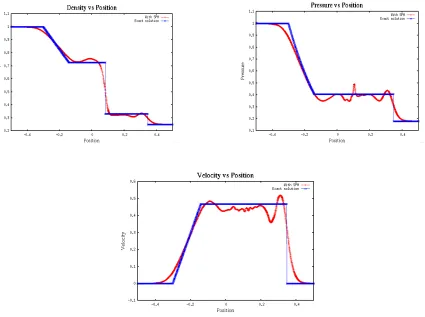
7.1.2.2 Energy evolution technique with AV (Standard SPH method)

(46)

[image:46.612.96.521.70.387.2]

7.1. Analysis 37

Figure 7.4: Plots of density, velocity and pressure versus position for energy evolution technique with AV using standard SPH equations at t=0.18

7.1.2.3 Energy evolution technique with AV (2nd Method)

(47)

[image:47.612.200.394.74.216.2]

38 Chapter 7. Results and Analysis

Figure 7.5: Plots of density, velocity and pressure versus position for energy evolution technique with AV using SPH methods inspired from Riemann solvers at t=0.18

7.2

Results

7.2.1

Shock tube without AV

Figure 7.1 and 7.2 show us that, irrespective of the evolution technique used, we have

to use Artificial Viscosity when we are evolving the system. The oscillations seen in the

figures are due to the absence of AV.

7.2.2

Shock tube with AV

We have used entropy evolution technique in the figure 7.3 and standard SPH energy

evolution for figure 7.4. We got rid of most of the oscillations, However the second

energy evolution technique gives better results in terms of resembling the exact solutions

(48)

Chapter 8

Conclusions and Future Work

8.1

Conclusions

In this project we have done the following

• Studied the basic formulation of Smoothed Particle Hydrodynamics.

• Studied different integration techniques and used it in expanding the SPH code

StarCrash. From the analysis we can conclude that Leap Frog, RK2 and RK4

methods give substantially better conservation of energy in comparison to the Euler

Technique.

• Studied the Sod shock tube test and used it for studying the different methods

of evolving the SPH equations using artificial viscosity (AV). We were able to

numerically solve the shock tube test and produce results close to the analytical

solution by turning on AV.

• Studied different methods of evolving the shock tube using either change in entropy

or energy. In conclusion we can use either of the two methods for evolving a

non-relativistic system. We can either use the thermodynamical approach, if we want to

automatically satisfy the second law of thermodynamics or use the energy approach,

if we want to conserve the energy better. However, the results from both the energy

evolution techniques matched the exact solution much better than the results from

the entropy evolution technique.

• Studied two different time evolution techniques, which use the change in energy.

(49)

40 Chapter 8. Conclusions and Future Work

As one of the technique is similar to relativistic approach of SPH, we have built a

foundation for expanding the SPH code and using it to simulate relativistic systems.

8.2

Future Work

We have studied and used (in the code StarCrash) the energy evolution technique of

SPH which closely resembles the relativistic form of SPH proposed by (Rosswog, 2009).

For future work, we can add general relativistic SPH equations to the existing SPH code

StarCrash in which the space time metric can be considered un-perturbed by the self

gravity of the fluid. Relativistic SPH would be useful for studying of ejecta with rapidly

changing spatial geometries (for example tidal disruption of a star around a black hole)

and hydrodynamical systems with slowly varying gravitational fields, like post - merger

(50)

Bibliography

D. S. Balsara. von Neumann stability analysis of smooth particle hydrodynamics–

suggestions for optimal algorithms. Journal of Computational Physics, 121:357–372,

1995.

W. Benz, R. L. Bowers, A. G. W. Cameron, and W. H. . Press. Dynamic mass exchange

in doubly degenerate binaries. I - 0.9 and 1.2 solar mass stars. Astrophysical Journal,

348:647–667, jan 1990.

D. B. Bowen, M. Campanelli, J. H. Krolik, V. Mewes, and S. C. Noble. Relativistic

Dynamics and Mass Exchange in Binary Black Hole Mini-disks.Astrophysical Journal,

838:42, March 2017.

B.P. Abbott et al. Observation of gravitational waves from a binary black hole merger.

Phys. Rev. Lett., 116:061102, Feb 2016.

E.J. Caramana, M.J. Shashkov, and P.P. Whalen. Formulations of artificial viscosity for

multi-dimensional shock wave computations. Journal of Computational Physics.

J. A. Faber and F. A. Rasio. Post-Newtonian SPH calculations of binary neutron star

coalescence. III. Irrotational systems and gravitational wave spectra. Phys. Rev. D, 65

(8):084042, April 2002.

J. A. Faber, P. Grandcl´ement, and F. A. Rasio. Mergers of irrotational neutron star

binaries in conformally flat gravity. Physical Review D, 69(12), June 2004.

Joshua A. Faber and Frederic A. Rasio. Post-newtonian sph calculations of binary neutron

star coalescence: Method and first results. Physics. Review. D, 62:064012, Aug 2000.

(51)

42 BIBLIOGRAPHY

Joshua A. Faber, Frederic A. Rasio, and Justin B. Manor. Post-newtonian smoothed

particle hydrodynamics calculations of binary neutron star coalescence. ii. binary mass

ratio, equation of state, and spin dependence. Phys. Rev. D, 63:044012, Jan 2001.

R. A. Gingold and J. J. Monaghan. Smoothed particle hydrodynamics - Theory and

application to non-spherical stars. Monthly Notices of the Royal Astronomical Society,

181:375–389, November 1977.

L. Hernquist and N. Katz. TREESPH - A unification of SPH with the hierarchical tree

method. Astrophysical Journal, 70:419–446, June 1989.

Charles Hirsch, editor. Numerical Computation of Internal &Amp; External Flows:

Fun-damentals of Numerical Discretization. John Wiley & Sons, Inc., New York, NY, USA,

1988. ISBN 0-471-91762-1.

Randall J. LeVeque. Numerical methods for conservation laws (2. ed.). Lectures in

mathematics. Birkh¨auser, 1992. ISBN 978-3-7643-2723-1.

L. B. Lucy. A numerical approach to the testing of the fission hypothesis. Astronomical

Journal, 82:1013–1024, dec 1977.

J. J. Monaghan. On the problem of penetration in particle methods. Journal of

Compu-tational Physics, 82:1–15, May 1989.

J. J. Monaghan. Smoothed particle hydrodynamics. Annual reviews of Astronomy and

Astrophysics, 30:543–574, 1992.

J. J. Monaghan. SPH and Riemann Solvers. Journal of Computational Physics, 136:

298–307, September 1997.

M. Ponce. PhD thesis, Rochester Institute of technology. 2011.

D. J. Price. Modelling discontinuities and Kelvin Helmholtz instabilities in SPH. Journal

of Computational Physics, 227:10040–10057, December 2008.

(52)

BIBLIOGRAPHY 43

F. A. Rasio and S. L. Shapiro. Hydrodynamical evolution of coalescing binary neutron

stars. Astrophysical Journal, 401:226–245, December 1992.

F. A. Rasio and S. L. Shapiro. Hydrodynamics of binary coalescence. 1: Polytropes with

stiff equations of state. Astrophysical Journal, 432:242–261, September 1994.

F. A. Rasio and S. L. Shapiro. Hydrodynamics of binary coalescence. 2: Polytropes with

gamma = 5/3. Astrophysica, 438:887–903, January 1995.

S. Rosswog. Astrophysical smooth particle hydrodynamics. New Astronomy Reviews, 53:

78–104, April 2009.

S. Rosswog. SPH Methods in the Modelling of Compact Objects. Living Reviews in

Computational Astrophysics, 1:1, October 2015.

M. J. Valtonen, H. J. Lehto, and H. Pietil¨a. Probing the jet in the binary black hole

model of the quasar OJ287.Astronomy and Astrophysics, 342:L29–L31, February 1999.

J. Von Neumann and R. D. Richtmyer. A Method for the Numerical Calculation of

Theses

Smoothed Particle Hydrodynamics

Rochester Institute of Technology

SMOOTHED PARTICLE

ASTROPHYSICAL SCIENCES AND TECHNOLOGY

CERTIFICATE OF APPROVAL

Dr. Nathaniel Barlow, Committee Member

Contents

List of Figures

Chapter 1

Chapter 2

Advantages and disadvantages of smoothed

Theoretical development of SPH

The SPH kernel interpolation

The “vanilla ice” SPH equation

Different evolution techniques

Chapter 3

Basic equations used in StarCrash

Artificial Viscosity

First law of thermodynamics

The gravity solver

Leap-frog technique

Number of Neighbours

Chapter 4

Euler’s Method

Leap Frog

Runge - Kutta Second order (RK2)

Runge - Kutta Fourth Order (RK4)

Chapter 5

Physical description of the shock tube problem

Analysis of the shock tube problem

Euler equation of gas dynamics

Exact solution

Artificial Viscosity

Chapter 6

Standard SPH Viscosity

New form of AV technique

Chapter 7

Shock tube with AV

Results

Chapter 8

Future Work

Bibliography

42 BIBLIOGRAPHY

BIBLIOGRAPHY 43