AIMS’ Journals
VolumeX, Number0X, XX200X pp.X–XX
STABILISATION BY DELAY FEEDBACK CONTROL FOR
HIGHLY NONLINEAR HYBRID STOCHASTIC DIFFERENTIAL
EQUATIONS
Zhenyu Lu
School of Electronic and Information Engineering Nanjing University of Information Science and Technology
Nanjing, Jiangsu 210044, China
Junhao Hu
∗School of Mathematics and Statistics South-Central University for Nationalities
Wuhan, Hubei 430074, China Xuerong Mao
Department of Mathematics and Statistics University of Strathclyde, Glasgow G1 1XH, U.K.
(Communicated by the associate editor Professor T. Caraballo)
Abstract. Given an unstable hybrid stochastic differential equation (SDE, also known as an SDE with Markovian switching), can we design adelay feed-back control to make the controlled hybrid SDE become asymptotically stable? The paper [14] by Mao et al. was the first to study the stabilisation by de-lay feedback controls for hybrid SDEs, though the stabilization bynon-delay
feedback controls had been well studied. A critical condition imposed in [14] is that both drift and diffusion coefficients of the given hybrid SDE need to satisfy the linear growth condition. However, many hybrid SDE models in the real world do not fulfill this condition (namely, they are highly nonlinear) and hence there is a need to develop a new theory for these highly nonlinear SDE models. The aim of this paper is to designdelayfeedback controls in order to stabilise a class of highly nonlinear hybrid SDEs whose coefficients satisfy the polynomial growth condition.
1. Introduction. Hybrid stochastic differential equations (SDEs) driven by continuous-time Mar-kov chains (also known as SDEs with MarMar-kovian switching) have frequently been used in many branches of science and industry. The hybrid SDEs can be described by
dx(t) =f(x(t), r(t), t)dt+g(x(t), r(t), t)dB(t). (1.1) Here the statex(t) takes values in Rn and the mode r(t) is a Markov chain taking values in a
finite spaceS={1,2,· · ·, N},B(t) is a Brownian motion andf andgare referred to as the drift
2010Mathematics Subject Classification. Primary: 60H10, 60J10; Secondary: 93D15.
Key words and phrases. Brownian motion, Markov chain, Asymptotic stability, Lypunov functional.
The authors would like to thank the Royal Society (WM160014, Royal Society Wolfson Re-search Merit Award), the Royal Society and the Newton Fund (NA160317, Royal Society-Newton Advanced Fellowship), the Royal Society of Edinburgh (61294), the EPSRC (EP/K503174/1), the Natural Science Foundation of China (61773220, 61473334, 61876192, 61374085), the Ministry of Education (MOE) of China (MS2014DHDX020) for their financial support.
∗Corresponding author: J. Hu.
and diffusion coefficient, respectively. One of the important issues in the study of hybrid SDEs is the analysis of stability (see, e.g., [4,6,15,17,20,21,23]). In particular, [12] is one of most cited papers (more than 560 Google citations) while [16] is the first book in this area (more than 800 Google citations).
Given an unstable hybrid SDE in the form of (1.1), it is classical to find a feedback control
u(x(t), r(t), t), based on the current statex(t), for the controlled system
dx(t) = [f(x(t), r(t), t) +u(x(t), r(t), t)]dt+g(x(t), r(t), t)dB(t) (1.2) to become stable. However, taking into account a time lagτ (>0) between the time when the observation of the state is made and the time when the feedback control reaches the system, it is more realistic that the control depends on a past statex(t−τ). Accordingly, the control should be of the form u(x(t−τ), r(t), t). Hence, the stabilisation problem becomes to design a delay feedback controlu(x(t−τ), r(t), t) for the controlled system
dx(t) = [f(x(t), r(t), t) +u(x(t−τ), r(t), t)]dt+g(x(t), r(t), t)dB(t) (1.3) to be stable. Mao et al. were the first to study this stabilisation problem in [14] by the delay feedback control for hybrid SDEs and there have been some further developments since then (see, e.g., [13,22]), although the method of delay feedback controls has been well used in the area of ordinary differential equations (see, e.g., [1,3,19]). The common restrict condition imposed in these existing papers in the area of hybrid SDEs is that both drift coefficientf and diffusion one
g need to satisfy the linear growth condition (namely bounded by linear functions). It is this restrict condition that excludes many SDE models in the real world, for example, the following scalar hybrid SDE
dx(t) =f(x(t), r(t), t)dt+g(x(t), r(t), t)dB(t), (1.4) where the coefficientsf andgare defined by
f(x,1, t) =x−3x3, f(x,2, t) =x−x3, g(x,1, t) =x2, g(x,2, t) = 0.5x2, (1.5)
B(t) is a scalar Brownian motion,r(t) is a Markov chain on the state spaceS={1,2}with its generator
Γ =
−1 1
5 −5
. (1.6)
This is a simple version of hybrid SDE models appeared frequently in finance and population systems (see, e.g., [2,8]). It is therefore necessary and important to establish a new theory which shows how to design delay feedback controls in order to stabilise highly nonlinear hybrid SDEs. Let us begin to establish our new theory.
2. Notation. Throughout this paper, unless otherwise specified, we use the following notation. IfAis a vector or matrix, its transpose is denoted byAT. Forx∈Rn,|x|denotes its Euclidean
norm. IfAis a matrix, we let|A|=ptrace(ATA) be its trace norm. IfAis a symmetric
real-valued matrix (A=AT), denote by λmin(A) and λmax(A) its smallest and largest eigenvalue,
respectively. ByA≤0 andA <0, we meanAis non-positive and negative definite, respectively. LetR+ = [0,∞). Forh > 0, denote by C([−h,0];Rn) the family of continuous functions ϕ
from [−h,0]→Rn with the normkϕk= sup
−h≤u≤0|ϕ(u)|. If botha, bare real numbers, then a∧b= min{a, b}anda∨b= max{a, b}. IfAis a subset of Ω, denote byIAits indicator function; that is,IA(ω) = 1 ifω∈Aand 0 otherwise.
Let (Ω,F,{Ft}t≥0,P) be a complete probability space with a filtration{Ft}t≥0satisfying the
usual conditions (i.e. it is increasing and right continuous whileF0 contains allP-null sets). Let B(t) = (B1(t),· · ·, Bm(t))T be an m-dimensional Brownian motion defined on the probability
space. Letr(t),t≥0, be a right-continuous Markov chain on the probability space taking values in a finite state spaceS={1,2,· · ·, N}with generator Γ = (γij)N×N given by
P{r(t+ ∆) =j|r(t) =i}= (
γij∆ +o(∆) ifi6=j,
1 +γii∆ +o(∆) ifi=j,
where ∆>0. Hereγij≥0 is the transition rate fromitoj ifi6=jwhile
γii=−X
j6=i γij.
simple jumps in any finite subinterval ofR+. We stress that almost all sample paths ofr(t) are right continuous.
Suppose that the underlying system is described by a nonlinear hybrid SDE
dx(t) =f(x(t), r(t), t)dt+g(x(t), r(t), t)dB(t) (2.1) ont≥0 with the initial valuex(0) =x0∈Rn, where
f:Rn×S×R+→Rn and g:Rn×S×R+→Rn×m
are Borel measurable functions. The classical conditions for the existence and uniqueness of the global solution are the local Lipschitz condition and the linear growth condition (see, e.g., [9,10,11,16]). In this paper, we need the local Lipschitz condition. However, we will consider highly nonlinear hybrid SDEs which, in general, do not satisfy the linear growth condition in this paper. We therefore impose the polynomial growth condition, instead of the linear growth condition. Let us state these conditions as an assumption for the use of this paper.
Assumption 2.1. Assume that for any real numberb >0, there exists a positive constant Kb
such that
|f(x, i, t)−f(¯x, i, t)| ∨ |g(x, i, t)−g(¯x, i, t)| ≤Kb(|x−x¯|) (2.2)
for allx,x¯∈Rnwith|x| ∨ |x¯| ≤band all(i, t)∈S×R+. Assume moreover that there exist three
constantsK >0,q1≥1andq2≥1such that
|f(x, i, t)| ≤K(1 +|x|q1) and |g(x, i, t)| ≤K(1 +|x|q2) (2.3) for all(x, i, t)∈Rn×S×R+.
Of course, ifq1=q2= 1 then condition (2.3) is the familiar linear growth condition. However, let us stress once again that we are here interested in hybrid SDEs without the linear growth condition. In other words, we will either haveq1>1 orq2>1. We will refer to condition (2.3) as the polynomial growth condition.
Let us now suppose that the given SDE (2.1) is unstable and we are required to design a delay feedback controlu(x(t−τ), r(t), t) in the drift part so that the controlled system
dx(t) = [f(x(t), r(t), t) +u(x(t−τ), r(t), t)]dt+g(x(t), r(t), t)dB(t), t≥0, (2.4) becomes stable. Of course, we assume that the controller functionu(x, i, t) is a Borel measurable function and is locally Lipschitz inx. This controlled system is a hybrid stochastic differential delay equation (SDDE). For an SDDE, it is required to know the initial datax(t) ont∈[−τ,0] in order for its solution to be well defined, although the given SDE (2.1) is non-delay and it only requires the initial value x(0) ∈ Rn. This can be interpreted as follows: the underlying
equation (2.1) evolved from before, say from time−τ, and we have observed the whole segment {x(t) :−τ ≤t≤0}by the current timet= 0. Starting from time zero on, we will then design the feedback controlu(x(t−τ), r(t), t) to stabilise the hybrid system. We can hence impose the initial data
{x(t) :−τ≤t≤0}=ξ∈C([−τ,0];Rn) andr(0) =r0∈S. (2.5) It is known that Assumption2.1 only guarantees that the hybrid SDDE (2.4) has a unique maximal local solution, which may explode to infinity at a finite time (see, e.g., [16]). To avoid such a possible explosion, we need to impose an additional condition in terms of Lyapunov functions. For this purpose, we need more notation.
LetC2,1(Rn×S×R+;R+) denote the family of non-negative functionsU(x, i, t) defined on
(x, i, t)∈Rn×S×R+ which are continuously twice differentiable inxand once int. For such a
functionU(x, i, t), we will let
Ut(x, i, t) = ∂U(x, i, t)
∂t , Ux(x, i, t) =
∂U(x, i, t) ∂x1 ,· · ·,
∂U(x, i, t)
∂xn
,
and
Uxx(x, i, t) =∂
2U(x, i, t) ∂xk∂xl
n×n.
LetC(Rn×[−τ,∞);R+) denote the family of all continuous functions fromRn×[−τ,∞) toR+. For a givenU∈C2,1(Rn×S×R+;R+), we define a functionLU:Rn×S×R+→Rby
LU(x, i, t) =Ut(x, i, t) +Ux(x, i, t)f(x, i, t)
+1 2trace[g
T(x, i, t)Uxx(x, i, t)g(x, i, t)] + N X
j=1
Please note thatLUis a single function (notLacting onU) associated with the given SDE (2.1) but not the controlled SDDE. We can now state another assumption.
Assumption 2.2. Assume that there exists a pair of functionsU¯∈C2,1(Rn×S×R+;R+)and
¯
U1∈C(Rn×[−τ,∞);R+), as well as three constantsc1>0,c2∈(0,1)andq≥2(q1∨q2)(where q1andq2 are the same as in Assumption2.1), such that
|x|q≤U¯(x, i, t)≤U1¯ (x, t) ∀(x, i, t)∈Rn×S×R+ (2.7)
and
LU¯(x, i, t) + ¯Ux(x, i, t)u(y, i, t)≤c1−U1¯ (x, t) +c2U1¯ (y, t−τ) (2.8)
for all(x, y, i, t)∈Rn×Rn×S×R+.
Let us now cite a theorem from [4], which shows the unique global solution of the SDDE (2.4) and itsq-th moment property under the above assumptions.
Theorem 2.3. Under Assumptions2.1and2.2, the SDDE (2.4) with the initial data (2.5) has the unique global solutionx(t)ont≥ −τand the solution has the property that
sup −τ≤t<∞E
|x(t)|q<∞. (2.9)
This theorem implies a number of nice properties of the solution. For example, for anyt≥0,
x(t) is bounded inLp for anyp ∈ (0, q] while bothf(x(t), r(t), t) andg(x(t), r(t), t) are in L2.
These properties will play their fundamental roles when we discuss the stabilisation of the SDDE (2.4) in the next section. Assumptions2.1and2.2will form our standing hypotheses in this paper. Let us emphasise that we will NOT explicitly mention Assumptions2.1and2.2in the next section in order for us to concentrate on our new assumptions to be imposed.
For the stability purpose of this paper, we naturally assume that
f(0, i, t)≡0, u(0, i, t)≡0, g(0, i, t)≡0 (2.10) for all (i, t)∈S×R+. So the SDDE (2.4) admits a trivial solutionx(t)≡0.
3. Stabilisation. In this section, we will use the method of Lyapunov functionals to investigate the asymptotic stability of the controlled SDDE (2.4). To define a Lyapunov functional for the use of this paper, we define two segments ˆxt :={x(t+s) :−2τ ≤s≤0}and ˆrt:= {r(t+s) : −2τ≤s≤0}fort≥0. For ˆxtand ˆrtto be well defined for 0≤t <2τ, we setx(s) =ξ(−τ) for
s∈[−2τ,−τ) andr(s) =r0 fors∈[−2τ,0). The Lyapunov functional used in this paper will be of the form
V(ˆxt,ˆrt, t) =U(x(t), r(t), t)
+θ Z0
−τ Z t
t+s h
τ|f(x(v), r(v), v) +u(x(v−τ), r(v), v)|2+|g(x(v), r(v), v)|2idvds (3.1)
fort≥0, whereU∈C2,1(Rn×S×R+;R+) andθis a positive number to be determined later
while we set
f(x, i, v) =f(x, i,0), u(x, i, v) =u(x, i,0), g(x, i, v) =g(x, , i,0)
for (x, i, v)∈Rn×S×[−2τ,0). The following lemma shows thatV(ˆxt,ˆrt, t) is an Itˆo process.
Lemma 3.1. With the notation above,V(ˆxt,ˆrt, t)is an Itˆo process ont≥0with its Itˆo differ-ential
dV(ˆxt,ˆrt, t) =LV(ˆxt,rt, tˆ )dt+dM(t), (3.2)
whereM(t)is a continuous local martingale withM(0) = 0and
LV(ˆxt,rt, tˆ )
=LU(x(t), r(t), t) +Ux(x(t), r(t), t)u(x(t−τ), r(t), t)
+θτhτ|f(x(t), r(t), t) +u(x(t−τ), r(t), t)|2+|g(x(t), r(t), t)|2i
−θ Z t
t−τ h
Proof. Regarding the solutionx(t) of equation (2.4) as an Itˆo process and applying the generalised Itˆo formula (see, e.g., [16]) toU(x(t), r(t), t), we get
dU(x(t), r(t), t) =
LU(x(t), r(t), t) +Ux(x(t), r(t), t)u(x(t−τ), r(t), t)
dt+dM(t), (3.4) fort≥0, whereM(t) is a continuous local martingale withM(0) = 0 (the explicit form ofM(t) is of no use in this paper so we do not state it here but it can be found in [16, Theorem 1.45 on page 48]) and the functionLUhas been defined in Section 2. On the other hand, the fundamental theory of calculus shows
d Z 0
−τ Z t
t+s h
τ|f(x(v), r(v), v) +u(x(v−τ), r(v), v)|2+|g(x(v), r(v), v)|2idvds
=
τ
h
τ|f(x(t), r(t), t) +u(x(v−τ), r(v), v)|2+|g(x(t), r(t), t)|2i
−
Z t
t−τ h
τ|f(x(v), r(v), v) +u(x(v−τ), r(v), v)|2+|g(x(v), r(v), v)|2idvdt. (3.5)
Applying the generalised Itˆo formula (see, e.g., [16]) to the Lyapunov functional defined by (3.1) and using (3.4) and (3.5), we then get the required assertion (3.3).
To study the asymptotic stability of the controlled SDDE (2.4), we need to impose a couple of new assumptions. First of all, recall that the delayτis the time lag between the time when the observation of the state is made and the time when the feedback control reaches the system. If there is no time lag, namely the feedback control acts instantly when the state observation is made, then the controlled SDDE (2.4) becomes the controlled SDE (1.2) (the classical one). This indicates that the feedback control should at least be able to make the SDE (1.2) asymptotically stable and henceLU(x, i, t) +Ux(x, i, t)u(x, i, t) should be negative-definite. However, our underlying controlled system is a highly nonlinear SDDE. To cope with the effect of the time lag and high nonlinearity, we need to impose a stronger assumption.
Assumption 3.2. Assume that there is a function U ∈C2,1(Rn×S×R+;R+)and positive
constantsβj,j= 0,1,2,3, such that
LU(x, i, t) +Ux(x, i, t)u(x, i, t) +β1|Ux(x, i, t)|2
+β2|f(x, i, t)|2+β3|g(x, i, t)|2≤ −β0|x|2 (3.6)
for all(x, i, t)∈Rn×S×R+.
We next compare our controlled SDDE (2.4) with the SDE (1.2) and observe that it is the differenceu(x(t), r(t), t)−u(x(t−τ), r(t), t) which makes the two controlled systems different. However, if the time lagτis sufficiently small, we may hope the differenceu(x(t), r(t), t)−u(x(t−
τ), r(t), t) could be so small that the SDDE (2.4) remains stable and this would be the case if
u(x, i, t) is uniformly continuous inx. This motivates us to impose the other assumption in this section.
Assumption 3.3. Assume that there exists a positive numberβsuch that
|u(x, i, t)−u(y, i, t)| ≤β|x−y| (3.7)
for allx, y∈Rn,i∈Sandt≥0.
This assumption, together with (2.10), implies
|u(x, i, t)| ≤β|x|, ∀(x, i, t)∈Rn×S×R+. (3.8)
Theorem 3.4. Let Assumptions3.2and3.3hold. Assume also that
τ <
√
β0β1
β2 and τ≤
√
β1β2 β ∧
2β1β3
β2 . (3.9)
Then for any given initial data (2.5), the solution of the SDDE (2.4) has the property that Z ∞
0
E|x(t)|2dt <∞. (3.10)
That is, the controlled SDDE (2.4) isH∞-stable inL2.
Proof. Fix the initial dataξ∈C([−τ,0];Rn) andr0∈Sarbitrarily. Letk0 >0 be a sufficiently
large integer such thatkξk< k0. For each integerk≥k0, define the stopping time
where throughout this paper we set inf∅=∞(as usual∅denotes the empty set). It is easy to see, by Theorem2.3, thatζkis increasing to infinity with probability 1 ask→ ∞. By the generalised Itˆo formula (see, e.g., [16, Lemma 1.9 on page 49]), we obtain from Lemma3.1that
EV(ˆxt∧ζk,ˆrt∧ζk, t∧ζk) =V(ˆx0,r0,ˆ 0) +E
Z t∧ζk
0 L
V(ˆxs,ˆrs, s)ds (3.11)
for anyt≥0 andk≥k0.
We now letθ=β2/(2β1). (Please recall thatθis the free parameter in the definition of the Lyapunov functional.) By Assumption3.3, it is easy to see that
Ux(x(t), r(t), t)[u(x(t−τ), r(t), t)−u(x(t), r(t), t)]
≤β1|Ux(x(t), r(t), t)|2+ β2
4β1|x(t)−x(t−τ)|
2. (3.12)
By condition (3.9), we also have
2θτ2≤β2 and θτ≤β3. (3.13)
It then follows from Lemma3.1that
LV(ˆxs,ˆrs, s)
≤LU(x(s), r(s), s) +Ux(x(s), r(s), s)u(x(s), r(s), s) +β1|Ux(x(s), r(s), s)|2
+β2|f(x(s), r(s), s)|2+ 2θτ2|u(x(s−τ), r(s), s)|2+β3|g(x(s), r(s), s)|2
+ β
2
4β1|x(s)−x(s−τ)| 2
− β
2
2β1 Z s
s−τ h
τ|f(x(v), r(v), v) +u(x(v−τ), r(v), v)|2+|g(x(v), r(v), v)|2idv.
By Assumption3.2and inequality (3.8), we then have
LV(ˆxs,ˆrs, s)
≤ −β0|x(s)|2+ 2θτ2β2|x(s−τ)|2+ β2
4β1|x(s)−x(s−τ)| 2
− β
2
2β1 Z s
s−τ h
τ|f(x(v), r(v), v) +u(x(v−τ), r(v), v)|2+|g(x(v), r(v), v)|2idv.
Substituting this into (3.11) implies
EV(ˆxt∧ζk,rtˆ∧ζk, t∧ζk)≤V(ˆx0,ˆr0,0) + Ψ1+ Ψ2−Ψ3, (3.14) where
Ψ1=E Z t∧ζk
0
−β0|x(s)|2+ 2θτ2β2|x(s−τ)|2 ds,
Ψ2= β2
4β1E Z t∧ζk
0
|x(s)−x(s−τ)|2ds,
Ψ3= β2
2β1E Z t∧ζk
0
Z s
s−τ h
τ|f(x(v), r(v), v) +u(x(v−τ), r(v), v)|2
+|g(x(v), r(v), v)|2idvds.
Noting that
Z t∧ζk
0
|x(s−τ)|2ds≤ Z t∧ζk
−τ
|x(s)|2ds,
we have
Ψ1≤2θτ3β2kξk2−(β0−2θτ2β2)E Z t∧ζk
0
|x(s)|2ds, (3.15)
Substituting this into (3.14) and recalling (3.1), we obtain
EU(x(t∧ζk), r(t∧ζk), t∧ζk) + (β0−2θτ2β2)E Z t∧ζk
0
|x(s)|2ds≤C1+ Ψ
whereC1=V(ˆx0,ˆr0,0) + 2θτ3β2kξk2. Applying the well-known Fatou lemma and recalling the
paragraph below Theorem2.3, we can letk→ ∞in (3.16) to get
(β0−2θτ2β2)E Zt
0
|x(s)|2ds≤C1+ ¯Ψ2−Ψ¯3, (3.17)
where
¯ Ψ2=
β2
4β1E Z t
0
|x(s)−x(s−τ)|2ds, ,
¯ Ψ3=
β2
2β1E Z t
0 Z s
s−τ h
τ|f(x(v), r(v), v) +u(x(v−τ), r(v), v)|2
+|g(x(v), r(v), v)|2idvds.
But, by the well-known Fubini theorem,
¯ Ψ2=
β2
4β1 Zt
0 E
|x(s)−x(s−τ)|2ds.
Fort∈[0, τ], we clearly have
¯ Ψ2≤
β2
2β1 Z τ
0
(E|x(s)|2+E|x(s−τ)|2)ds≤τ β 2
β1
sup −τ≤v≤τE
|x(v)|2
=:C2,
where, as usual, =: means ’denoted by’. Fort > τ, we have
¯
Ψ2≤C2+ β2
4β1 Z t
τ
E|x(s)−x(s−τ)|2ds.
On the other hand, it follows from the SDDE (2.4) that, fors≥τ,
E|x(s)−x(s−τ)|2
=E
Z s
s−τ
[f(x(v), r(v), v) +u(x(v−τ), r(v), v)]dv+
Z s
s−τ
g(x(v), r(v), v)dB(v)
2
≤2E Z s
s−τ
τ|f(x(v), r(v), v) +u(x(v−τ), r(v), v)|2+|g(x(v), r(v), v)|2dv.
Hence
¯
Ψ2≤C2+ β2
2β1 Z t
τ E Zs
s−τ h
τ|f(x(v), r(v), v) +u(x(v−τ), r(v), v)|2
+|g(x(v), r(v), v)|2idvds
≤C2+ β
2
2β1E Z t
0 Zs
s−τ h
τ|f(x(v), r(v), v) +u(x(v−τ), r(v), v)|2
+|g(x(v), r(v), v)|2i dvds
=C2+ ¯Ψ3,
where the Fubini theorem has been used once again. In other words, we always have ¯
Ψ2≤C2+ ¯Ψ3, ∀t≥0. (3.18)
Substituting this into (3.17) yields
(β0−2θτ2β2)E Z t
0
|x(s)|2ds≤C1+C2. (3.19)
Noting thatβ0−2θτ2β2=β0−β4τ2/β1>0 by condition (3.9), we see from the above inequality
that
E Z t
0
|x(s)|2ds≤ C1+C2 β0−β4τ2/β1.
Lettingt→ ∞and then using the Fubini theorem we obtain the assertion (3.10). The proof is therefore complete.
In general, it does not follow from (3.10) that limt→∞E|x(t)|2= 0. However, in our case, this
Theorem 3.5. Under the same assumptions of Theorem3.4, the solution of the controlled hybrid SDDE (2.4) satisfies
lim
t→∞E|x(t)|
2= 0
for any given initial data (2.5). That is, the controlled system (2.4) is asymptotically stable in mean square.
Proof. Fix the initial data (2.5) arbitrarily. By Theorem2.3and conditions (2.3) and (3.8), we can apply the Itˆo formula to show
E|x(t2)|2−E|x(t1)|2
=
E
Zt2
t1
2x(t)[f(x(t), r(t), t) +u(x(t−τ), r(t), t)] +|g(x(t), r(t), t)|2dt
≤C3(t2−t1),
whereC3is a constant independent oft1 andt2. That is,E|x(t)|2 is uniformly continuous inton R+. It then follows from (3.10) that limt→∞E|x(t)|2= 0 as required.
In general, we cannot imply limt→∞|x(t)|= 0 a.s. from (3.10). But, in our case, this is once again possible with an additional condition. We should also point out that You et al. [22] showed thisunder the linear growth conditionon the coefficients of the underlying SDDE. Our new proof given below does not only overcome the difficulty without the linear growth condition but is also much simplified.
Theorem 3.6. In addition to the assumptions of Theorem3.4, assume that
lim
k→∞
inf{U(x, i, t) :|x| ≥k, (i, t)∈S×R+}=∞. (3.20)
Then the solution of the controlled hybrid SDDE (2.4) satisfies
lim
t→∞x(t) = 0 a.s. (3.21)
for any given initial data (2.5). That is, the controlled system (2.4) is almost surely asymptotically stable.
Proof. Again fix any initial data (2.5). We first observe that (3.10) is equivalent to that
C4:=E Z ∞
0
|x(t)|2dt <∞ (3.22)
by the well-known Fubini theorem. This implies thatR∞
0 |x(t)|
2dt <∞a.s. and hence
lim inf
t→∞ |x(t)|= 0 a.s. (3.23)
But this is not the required assertion (3.21) yet. Let us now assume that the assertion were not true. There is then a positive numberε∈(0,1/4) such that
P
lim sup
t→∞
|x(t)|>2ε
≥4ε. (3.24)
For eachk≥ kξk, letζkbe the same stopping time as defined in the proof of Theorem3.4and set
φk= inf{U(x, i, t) :|x| ≥k, (i, t)∈S×R+}.
It follows from (3.16) that
φkP(ζk≤t)≤C1+ Ψ2−Ψ3, ∀t≥0.
This, together with (3.18), implies lim sup
k→∞
φkP(ζk≤t)≤C1+C2, ∀t≥0. (3.25)
As this holds for anyt≥0, we must have lim sup
k→∞
φkP(ζk<∞)≤C1+C2.
Thus, there is a positive integerk1 large enough for
φkP(ζk<∞)≤C1+C2+ 1, ∀k≥k1.
We can then choose a particulark≥k1, which will be fixed from now on, sufficiently large for (C1+C2+ 1)/φk≤εto getP(ζk<∞)≤ε. This means that
Combining (3.24) and (3.26) together gives
P( ¯Ω)≥3ε, (3.27)
where ¯ Ω = n lim sup t→∞
|x(t)|>2εand|x(t)|< kfor∀t≥ −τ o
.
Define the stopped process ¯x(t) =x(t∧ζk) fort≥0. Clearly, ¯x(t) is an Itˆo process of the form
dx¯(t) = ¯f(t)dt+ ¯g(t)dB(t), (3.28) where
¯
f(t) = [f(x(t), r(t), t) +u(x(t−τ), r(t), t)]I[0,ζk)(t),
¯
g(t) =g(x(t), r(t), t)I[0,ζk)(t).
By Assumptions2.2,3.3as well as condition (2.10), we see that ¯f(t) and ¯g(t) are bounded processes, say
|f¯(t)| ∨ |¯g(t)| ≤C5 a.s. (3.29) for allt≥0. Let us now define a sequence of stopping times
µ1= inf{t≥0 :|x¯(t)| ≥2ε},
µ2l= inf{t≥µ2l−1:|x¯(t)| ≤ε}, l= 1,2,· · ·, µ2l+1= inf{t≥µ2l:|¯x(t)| ≥2ε}, l= 1,2,· · ·.
By (3.23) and the definition of ¯Ω, we have ¯
Ω⊂ {µl<∞}, l= 1,2,· · ·. (3.30)
Choose a small positive numberν and a large positive integer ¯lsuch that
C5(ν+ 4√2ν)≤ε2 and C4< ε3ν¯l. (3.31) By (3.27) and (3.30), we can further choose a sufficiently large numberT for
P(µ2¯l≤T)≥2ε. (3.32)
In particular, ifµ2¯l ≤T, |x¯(µ2¯l)|=εand henceµ2¯l < ζk by the definition of ¯x(t) (otherwise |¯x(µ2¯l)|=|x¯(ζk)|=k, a contradiction). In other words, we have
¯
x(t, ω) =x(t, ω) for all 0≤t≤µ2¯landω∈ {µ2¯l≤T}. (3.33)
By the Burkholder-Davis-Gundy inequality (see, e.g., [16, Theorem 2.13 on page 70]), we can then derive from (3.28) that, for 1≤l≤¯l,
E
sup
0≤t≤ν
|¯x(µ2l−1∧T+t)| − |x¯(µ2l−1∧T)|
≤E sup
0≤t≤ν
|x¯(µ2l−1∧T+t)−x¯(µ2l−1∧T)|
≤E
Z µ2l−1∧T+ν
µ2l−1∧T
|f¯(s)|ds+ 4√2E
Z µ2l−1∧T+ν
µ2l−1∧T
|¯g(s)|2ds1/2
≤C5(ν+ 4√2ν).
This, together with (3.31), implies
P
sup
0≤t≤ν
|¯x(µ2l−1∧T+t)| − |x¯(µ2l−1∧T)| ≥ε
≤ε.
Noting thatµ2l−1≤T ifµ2¯l≤T, we can derive from (3.32) and the above inequality that
P
{µ2¯l≤T} ∩ n
sup
0≤t≤ν
|x¯(µ2l−1+t)| − |x¯(µ2l−1)| < ε
o
=P(µ2¯l≤T)−P
{µ2¯l≤T} ∩ n
sup
0≤t≤ν
|x¯(µ2l−1∧T+t)| − |x¯(µ2l−1∧T)| ≥ε
o
≥P(µ2¯l≤T)−P
sup
0≤t≤ν
|x¯(µ2l−1∧T+t)| − |x¯(µ2l−1∧T)| ≥ε
≥ε.
This implies easily that
P
{µ2¯l≤T} ∩ {µ2l−µ2l−1≥ν}
Finally, by (3.22), (3.33) and (3.34), we derive
C4=E Z∞
0
|x(t)|2dt
≥
¯ l X
l=1 E
I{µ2¯l≤T}
Z µ2l
µ2l−1
|x¯(t)|2dt
≥ε2 ¯ l X
l=1 E
I{µ2¯l≤T}(µ2l−µ2l−1)
≥ε2ν ¯ l X
l=1 P
{µ2¯l≤T} ∩ {µ2l−µ2l−1≥ν}
≥ε3ν¯l.
But this contradicts the second inequality in (3.31). Therefore the required assertion (3.21) must hold. The proof is complete.
4. Examples. As pointed out in Section 1, our key aim in this paper is to design adelayfeedback control in order to stabilise a given unstable hybrid SDE whose drift and diffusion coefficients are highly nonlinear. As far as we know, the paper [14] by Mao et al. was the first to study the stabilisation bydelay feedback controls for hybrid SDEs and is the only paper on this topic so far. However, a critical condition imposed in [14] is that both drift and diffusion coefficients of the given unstable hybrid SDE need to satisfy the linear growth condition. Our new result in this paper has removed this restrictive condition, whence our new result enables us to design adelay
feedback control in order to stabilise a given unstable hybrid SDE. On the other hand, the use of our result depends on the construction of the Lyapunov functionU(x, i, t) and the control function
u(x, i, t) for conditions (3.6) and (3.7) to hold. We realise that, in general, there is no theory on the construction of the Lyapunov functions. Of course, this is not the problem of the Lyapunov method and, in fact, it is because there is no such a general theory that the Lyapunov method has been one of most powerful methods in the stability study for more than 100 years. Nevertheless, to apply our new result, we may first construct the Lyapunov functionU(x, i, t) and the control functionu(x, i, t) for the following hybrid SDE (not SDDE)
dx(t) = [f(x(t), r(t), t) +u(x(t), r(t), t)]dt+g(x(t), r(t), t)dB(t)
to be stable. There is a great amount of literature on hybrid SDEs (see, e.g., [16] and the reference therein). For our purpose, we need require that
LU(x, i, t) +Ux(x, i, t)u(x, i, t)≤ −β0|x|2
as well as (3.7) to hold. In order to overcome the high nonlinearity of the coefficientsf(x, i, t) andg(x, i, t), we may next modify them in order for them to satisfy the stronger condition (3.6). Finally, we just restrict the time delayτ sufficiently small for (3.9) to hold.
We should point out that the control functionu(x, i, t) used in this paper is allowed to depend on the modei(i.e., the state of the Markov chain). There are two reasons for this. One is because it is easier to design the control functionu(x, i, t), which is the key for our theory to be applied, if we take the different system structure in different mode into account. The other is because the underlying system may not be observable in some modes. In this case, the feedback control could not be used when the system are operating in those modes (namely we have to setu(x, i, t) = 0 for thosei) and the feedback control could only be designed for the other modes where the system is observable. This situation is illustrated in our Example4.2fully.
To illustrate our theoretical results, we return to the hybrid SDE (1.4), where the coefficients
f and gare defined by (1.5), B(t) is a scalar Brownian motion and r(t) is a Markov chain on
S={1,2}with the generator Γ defined by (1.6). As we mentioned in Section 1, this is a simple version of hybrid SDE models appeared frequently in finance and population systems (see, e.g., [2,8]). The reason why we use this simplified SDE model is not only to avoid the verification of the assumptions imposed becoming too long but also be able to illustrate our theory fully. We consider two cases.
given unstable hybrid SDE (1.4). In our notation, we assume that the controlled hybrid SDDE has the form
dx(t) = [f(x(t), r(t), t) +u(x(t−τ), r(t), t)]dt+g(x(t), r(t), t)dB(t) (4.1) while the delay feedback control is defined by
u(x(t−τ), r(t), t) =
−2x(t−τ) ifr(t) = 1,
−x(t−τ) ifr(t) = 2. (4.2) To apply our results in order to get the bound onτ, we need to verify the assumptions imposed in Sections 2 and 3. It is easy to see that Assumption2.1is satisfied withq1= 3 andq2= 2. To verify Assumption2.2, we define ¯U(x, i, t) =|x|6 for (x, i, t)∈R×S×R+. It is straightforward
to show that, for (x, y, i, t)∈R×R×S×R+,
LU¯(x, i, t) + ¯Ux(x, i, t)u(y, i, t) =
6x6−3x8−12x5y ifi= 1, 6x6−2.25x8−6x5y ifi= 2. Noting that 6x5y≤5x6+y6, we then have
LU¯(x, i, t) + ¯Ux(x, i, t)u(y, i, t)≤c1−4x6+ 2y6,
wherec1 = supx∈R
(20x6−3x8)∨(10x6−2.25x8)
<∞. That is, Assumption 2.2is fulfilled with ¯U1(x, t) = 4x6,c2= 0.5 andq= 6.
To verify Assumption3.2, we define
U(x, i, t) =
0.75(x2+x4) ifi= 1, x2+x4 ifi= 2
for (x, i, t)∈R×S×R+. It is easy to show that
LU(x, i, t) +Ux(x, i, t)u(x, i, t) =
−1.25x2−6.5x4−4.5x6 ifi= 1,
−1.25x2−3x4−2.5x6 ifi= 2.
Denote the left hand side of inequality (3.6) byLHS. Then
LHS=−1.25x2−6.5x4−4.5x6+β1(1.5x+ 3x3)2+β2(x−3x3)2+β3x4
=−(1.25−2.25β1−β2)x2−(6.5−9β1+ 6β2−β3)x4−(4.5−9β1−9β2)x6
wheni= 1, and
LHS=−1.25x2−3x4−2.5x6+β1(2x+ 4x3)2+β2(x−x3)2+ 0.25β3x4
=−(1.25−4β1−β2)x2−(3−16β1+ 2β2−0.25β3)x4−(2.5−16β1−β2)x6
wheni= 2. Choosingβ1=β2= 0.1 andβ3= 5.8, we obtain
LHS=
−
0.825x2−0.4x4−2.7x6 ifi= 1,
−0.75x2−0.15x4−0.8x6 ifi= 2.
Thus we always have
LHS≤ −0.75x2.
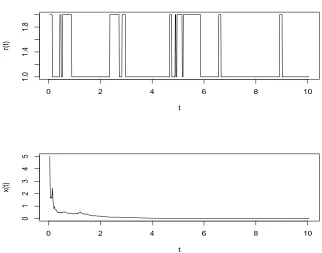
In other words, we have just verified Assumption 3.2with β0 = 0.75. Moreover, by definition (4.2) of the delay feedback control, we see easily that Assumption3.3holds withβ= 2. Finally, condition (3.9) becomesτ ≤0.06847. By Theorems3.4,3.5and 3.6, we can therefore conclude that if we use the delay feedback control (4.2) and make sure the time delayτ ≤0.06847, then the controlled hybrid SDDE (4.1) is not onlyH∞-stable inL2but also asymptotically stable in
L2and almost surely as well.
We perform a computer simulation with the time-delayτ= 0.06 for allt≥0 and the initial datax(u) = 5 + sin(u) foru∈[−0.06,0] andr(0) = 2. The sample paths of the Markov chain and the solution of the SDDE (4.1) are plotted in Figure 4.1. The simulation supports our theoretical results clearly.
Example 4.2. We now consider the case where the system is observable only in mode 1 but not in mode 2 so we could only use a delay feedback control in mode 1. In our notation, we assume that the controlled hybrid SDDE has the form of (4.1) and the delay feedback control is defined by
u(x(t−τ), r(t), t) =
−5x(t−τ) ifr(t) = 1,
0 ifr(t) = 2. (4.3)
0 2 4 6 8 10
1.0
1.4
1.8
t
r(t
)
0 2 4 6 8 10
0
1
2
3
4
5
t
x(t
[image:12.612.137.459.144.397.2])
Figure 4.1: The computer simulation of the sample paths of the Markov chain and the
SDDE (2.4) with control (4.2) and
τ
= 0.06 using the Euler–Maruyama method with
step size 10
−4.
Assumption2.2, we still define ¯U(x, i, t) =|x|6for (x, i, t)∈R×S×R+. It is straightforward to
show that, for (x, y, i, t)∈R×R×S×R+,
LU¯(x, i, t) + ¯Ux(x, i, t)u(y, i, t) =
6x6−3x8−30x5y ifi= 1,
(16x6−2.25x8)−10x6 ifi= 2.
Noting that 30x5y≤25x6+ 5y6, we then have
LU¯(x, i, t) + ¯Ux(x, i, t)u(y, i, t)≤c1−10x6+ 5y6,
wherec1 = supx∈R
(41x6−3x8)∨(16x6−2.25x8)
<∞. That is, Assumption 2.2is fulfilled with ¯U1(x, t) = 10x6,c2= 0.5 andq= 6.
To verify Assumption3.2, we define
U(x, i, t) =
0.25(x2+x4) ifi= 1, x2+x4 ifi= 2
for (x, i, t)∈R×S×R+. It is easy to show that
LU(x, i, t) +Ux(x, i, t)u(x, i, t) =
−1.25x2−4.5x4−1.5x6 ifi= 1, −1.75x2−1.5x4−2.5x6 ifi= 2. Still denote the left hand side of inequality (3.6) byLHS. Then
LHS=−1.25x2−4.5x4−1.5x6+β1(0.5x+x3)2+β2(x−3x)2+β3x4
=−(1.25−0.25β1−β2)x2−(4.5−β1+ 6β2−β3)x4−(1.5−β1−9β2)x6
wheni= 1, and
LHS=−1.75x2−1.5x4−2.5x6+β1(2x+ 4x3)2+β2(x−x3)2+ 0.25β3x4
wheni= 2. Choosingβ1=β2= 0.1 andβ3= 0.4 + 8√0.1), we obtain
LHS=
−1.125x2−(4.6−8√0.1)x4−0.5x6 ifi= 1, −1.25x2+ 2√0.1x4−0.8x6 ifi= 2.
As
−0.125x2+ 2√0.1x4−0.8x6=−0.125x2(1−16√0.1x2+ 6.4x4) =−0.125x2(1−8√0.1x2)2≤0,
we then always have
LHS≤ −1.125x2.
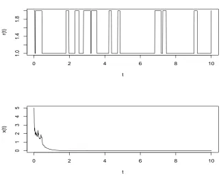
In other words, we have just verified Assumption3.2withβ0 = 1.125. Moreover, by definition (4.3) of the delay feedback control, we see easily that Assumption3.3holds withβ= 5. Finally, condition (3.9) becomesτ≤0.013416. By Theorems3.4,3.5and3.6, we can therefore conclude that if we use the delay feedback control (4.3) and make sure the time delayτ≤0.013416, then the controlled hybrid SDDE (2.4) is not onlyH∞-stable inL2 but also asymptotically stable in
L2and almost surely as well.
We should point out that with the delay feedback control (4.3), the controlled system (4.1) has its form
dx(t) = [x(t)−3x3(t)−5x(t−τ)]dt+x2(t)dB(t) in modei= 1, and
dx(t) = [x(t)−x3(t)]dt+ 0.5x2(t)dB(t)
in modei= 2. We observe that this controlled system is unstable in mode 2 while it is stable in mode 1 when the delayτ is sufficiently small. But, overall, the feedback controlled system (4.1) is stable as long asτ <0.013416.
We perform a computer simulation with the time-delayτ= 0.01 for allt≥0 and the initial datax(u) = 5 + sin(u) foru∈[−0.01,0] andr(0) = 2. The sample paths of the Markov chain and the solution of the SDDE (4.1) are plotted in Figure 4.2. The simulation supports our theoretical results.
5. Conclusion. In this paper we have discussed the stabilisation of highly nonlinear hybrid SDEs by delay feedback controls. We pointed out that the existing results on the stabilisation of nonlinear hybrid SDEs require the coefficients of the underlying SDEs satisfy the linear growth condition. On the other hand, many hybrid SDE models in the real world do not fulfill this linear growth condition (namely, they are highly nonlinear). There is hence a need to develop a new theory on the stabilisation by delay feedback controls for the highly nonlinear SDE models. In this paper we have successfully used the method of Lyapunov functionals to study this stabilisation problem by delay feedback controls. We have showed that a class of highly nonlinear unstable hybrid SDEs whose coefficients satisfy the polynomial growth condition can be stabilised by delay feedback controls. A couple of examples and computer simulations have been used to motivate our work and to illustrate our theory as well.
Acknowledgments. The authors wish to thank the referees for their detailed comments and helpful suggestions.
REFERENCES
[1] A. Ahlborn and U. Parlitz, Stabilizing unstable steady states using multiple delay deedback control,Physical Review Letters,93, 264101 (2004).
[2] A. Bahar and X. Mao, Stochastic delay population dynamics,Journal of International Applied Mathematics,11(4)(2004), 377–400.
[3] J. Cao, H.X. Li and D.W.C. Ho, Synchronization criteria of Lur’s systems with time-delay feedback control,Chaos, Solitons and Fractals,23(2005), 1285–1298.
[4] L. Hu, X. Mao and Y. Shen, Stability and boundedness of nonlinear hybrid stochastic differ-ential delay equations,Systems & Control Letters,62(2013), 178–187.
[5] G.S. Ladde and V. Lakshmikantham,Random Differential Inequalities, Academic Press, 1980. [6] Y. Ji and H.J. Chizeck, Controllability, stabilizability and continuous-time Markovian jump
linear quadratic control,IEEE Transaction on Automatic Control,35(1990), 777–788. [7] V.B. Kolmanovskii and V.R. Nosov,Stability of Functional Differential Equations, Academic
Press, 1986.
0 2 4 6 8 10
1.0
1.4
1.8
t
r(t
)
0 2 4 6 8 10
0
1
2
3
4
5
t
x(t
[image:14.612.137.460.143.398.2])
Figure 4.2: The computer simulation of the sample paths of the Markov chain and the
SDDE (2.4) with control (4.3) and
τ
= 0.01 using the Euler–Maruyama method with
step size 10
−4.
[9] X. Mao,Stability of Stochastic Differential Equations with Respect to Semimartingales, Long-man Scientific and Technical, 1991.
[10] X. Mao,Exponential Stability of Stochastic Differential Equations, Marcel Dekker, 1994. [11] X. Mao, Stochastic Differential Equations and Their Applications, 2nd edition, Horwood
Publishing Limited, Chichester, 2007.
[12] X. Mao, Stability of stochastic differential equations with Markovian switching,Stochastic Processes and Their Applications,79(1999), 45–67.
[13] X. Mao, Stabilization of continuous-time hybrid stochastic differential equations by discrete-time feedback control,Automatica,49(2013), 3677–3681.
[14] X. Mao, J. Lam and L. Huang, Stabilisation of hybrid stochastic differential equations by delay feedback control,Systems & Control Letters,57(2008), 927–935.
[15] X. Mao, A. Matasov and A.B. Piunovskiy, Stochastic differential delay equations with Mar-kovian switching,Bernoulli,6(2000), 73–90.
[16] X. Mao and C. Yuan,Stochastic Differential Equations with Markovian Switching, Imperial College Press, 2006.
[17] M. Mariton,Jump Linear Systems in Automatic Control, Marcel Dekker, 1990.
[18] S.-E.A. Mohammed,Stochastic Functional Differential Equations, Longman Scientific and Technical, 1984.
[19] K. Pyragas, Control of chaos via extended delay feedback,Physics Letters A,206(1995), 323–330.
[20] L. Shaikhet, Stability of stochastic hereditary systems with Markov switching, Theory of Stochastic Processes,2(1996), 180–184.
[22] S. You, W. Liu, J. Lu, X. Mao and Q. Qiu,, Stabilization of hybrid systems by feedback control based on discrete-time state observations, SIAM Journal on Control and Optimization,53
(2015), 905–925.
[23] D. Yue and Q. Han, Delay-dependent exponential stability of stochastic systems with time-varying delay, nonlinearity, and Markovian switching,IEEE Transaction on Automatic Con-trol,50(2005),217–222.
Received xxxx 20xx; revised xxxx 20xx.
E-mail address:Zhenyu Lu: [email protected]
E-mail address:Junhao Hu: [email protected]