1
Migration Estimation in India: A Monsoon Migration Model
Mr. Sandeep K. Rao
, Adjunct Faculty, PES University, PES-IUP, Bengaluru
2
Migration Estimation in India: A Monsoon Migration Model
Abstract
Rural-Urban and Rural-Rural migration has become one of the most common phenomenon of
population demographic changes. Several factors which contribute towards the improvement of
the livelihood and opportunities to the migrated labourers have been studied. More than 69 per
cent of the 1.21 billion people live in rural India (2011 Census) and agriculture is their main source
of income. Agriculture contributes to 18 per cent to the GDP of India. Due to the lack of adequate
public irrigation facilities most of these farmers are dependent heavily on monsoon as the main
source of water for agriculture. Since a large percentage of these farmers are into subsistence
farming, they lack the capital required to set up their own irrigation facilities. When the monsoon
fails, or when there is excess rain, there is loss of crop and hence rural-to-urban migration results.
There are many factors influencing rural to rural and rural to urban migration. One such important
factor is agricultural distress. Agriculture being predominantly dependent on monsoon in India,
there is an immediate need in accessing the relationship among agriculture, migration and rainfall.
This paper analyses the role of quantum of rainfall in determining the rate of migration with
empirical evidence from India and proposes a model to estimate the migration rate based on the
quantum of rainfall.
3
Introduction
Migration involves movement from one area to other, within or across the national administrative
boundaries for a specific short term period or for the purpose of permanent change in residence.
Migration can also be classified based on geographic boundaries like inter-state migration,
intra-state migration, inter-country or inter-continental migration. Moving across the national
boundaries occur as part of either immigration or as refugees. This has greater significance and
factors influencing cross border migration are diverse like natural disasters, wars, search of new
jobs and better living standards or opportunities.
In the coming decades, there can be disruptions in the human population and also the migration
due to changing climatic conditions. These climate-induced movements can have influences on
origin, destination and the path of migration. Rural-Urban migration spikes in India can occur due
to adverse economic conditions of the cultivators as a direct consequence of rainfall shortages.
(Bart, François Gemenne et.al, 2012). Large number of people are migrating due to the hostile
inhabitable conditions as a result of climate change (IOM, 2009).
Climate induced International migration has been studied with reference to the impact of the sea
level rise resulting in inundation of coastal regions. Arguments and questions were raised on the
institutional arrangements to handle such migrations both within the domestic boundaries and
across international borders (Byravan and Rajan, 2009). Studies have established the association
between low rainfall and international migration (Hunter et.al., 2013). Thirty per cent urban growth
in India is due to rural-urban migration (Mitra & Muryama, 2008), while two thirds of the urban
growth is due to migration around the world (Gugler, 1988).
4
migration (64th round of NSS Survey). The gross decadal intra state migration of male and female
in Karnataka state was 11.54 percent of its total urban population. The Bangalore Urban
Agglomeration was 13.4 percent, 16.4 percent in Delhi and 15.1 percent in Greater Mumbai (2001
Census). Bihar and Uttar Pradesh are the largest migrant origin states in India. Mumbai, Delhi and
Kolkata are the largest migrant destination cities in India. Drought prone rural regions of Andhra
Pradesh, Maharashtra, and Karnataka have seen significant seasonal migration in search of
employment with better wages. 32.76 percent of total migration in Karnataka, that is around
610,032 people migrated from rural to urban areas under all categories (2011 Census).
This paper focuses on Indian migration with respect to monsoon. In India, around 30 per cent of
the population migrate internally as per the Census of India, 2001, and around 28.5 per cent of the
population as per the NSSO 2007–08.
Literature Review
Climate change has become a major global concern in the recent decade. Several organisations
and world forums have debated on the impact of the changing climatic conditions on health,
farming, drought, natural calamities and others. One of the major emerging concern is the impact
of change in climate on the agricultural output. Studies have shown that there is a significant
impact of change in climate on agriculture (Kumar and Parikh, 2001; Mall et.al., 2006; World
Bank, 2008). The empirical evidence shows that the crop yields, especially those of cereals like
wheat and rice, have a significant drop with changing climatic conditions. This has also triggered
migration of people from agricultural sector. Thus there has been a lot of focus on the linkages
among weather variability, migration and urban-rural wage differentials (McLeman and Smit,
2006; Perch-Nielsen et al., 2008; Bardsley and Hugo, 2010; Feng et al.,2010, Dallman and
5
urban migration of farmers have also been studied (Wang, Rada et.al, 2014).
India has a large population which is dependent on the agriculture for their livelihood. Most of
these agricultural lands are rain fed due to the lack of irrigation infrastructure or inadequate capital
investments by farmers due to their low income status. Developing countries like India, is more
sensitive to rural-urban migration during extreme climatic and weather conditions which affect the
agricultural output. (McLeman and Hunter 2010). Short term migration is influenced by weather
variability, through the twenty-year total rainfall deviation and mean of maximum temperature
(Kavi Kumar and Brinda, 2012). There have been studies that indicate the migration under climate
change occurs either in the intra-national and/or intra-regional levels (Massey et al., 2010).
Other factors which affect the migration linked to agriculture, like the income status of the farmer,
has been studied. It is observed that farmers in the upper echelons of the socioeconomic spectrum
show lower sensitivity to climate induced migration as they have their own businesses, capital and
other assets which can provide them for longer periods. However, this is not true in case of lower
income status farmers (landless labourers), whose income is solely based on the agricultural
output. Adverse climate variations induce economic hardships to these farmers inducing rural to
rural or rural to urban migration. The cyclical migration for short durations may continue to grow
due to droughts. (Deshingkar and Start, 2003). Datt and Ravallion (1998), provide further
evidence of the productivity connection to migration through the estimation of effects on yield
growth on poverty, relative food prices and real wages in rural India between 1958-94. They
showed that poverty reduction is possible through both higher productivity and higher real wages.
Inhabitants of rural areas who are dependent highly on agriculture or natural resources for
subsistence are affected by lower rainfall and more intense weather patterns (McLeman and
6
to property damage as seen with events like storms, floods, earthquakes. They can also be slower
onset events like droughts which can lead to crop failure and depletion of productivity and yield.
(de Sherbinin, Warner, and Ehrhart 2011; Sanchez Cohen et al. 2012). Thus the lower yield leads
to lower household income. Complications can further compound where there is no adequate crop
insurance to cover the crop failure (Gine, Townsend, and Vickery 2008; Hertel and Rosch 2010).
More generally the families which are dependent on the natural resources face difficulties with
reduction in yields due to climate variability.
Models of Migration have been part of the literature which tries to establish the several
relationships among various factors influencing migration. Some important models are the
Ravenstein Law of migration (Ravenstein, 1885), Lee’s push pull Model (Lee, 1966), Gravity
model, Alonso’s General theory of movement (Vries et.al, 2000), Intervening opportunity model.
Several models have been developed and proposed which provides model framework for migration
linking it to environmental conditions (Perch-Nielsen et al., 2008; Black et al, 2011). In their
framework Black et.al., (2011) categorized economic factors, political factors, demographic
factors, social and environmental factors as the major drivers of migration. An agent based model
was developed to study the internal migration in Bangladesh. This model predicts that the internal
migrants over the next forty years may be in the range of three to ten million depending on the
extremity of the climatic changes (Hassani-Mahmooei and Parris, 2012). Various econometric
studies have established linkages of migration to weather variability through agriculture channel.
(Feng et.al., 2010; Barbieri et.al., 2010; Dillon et.al., 2011; and Marchiori et.al., 2012).
Warner, K., Afifi et.al, (2012), used the Rainfalls Agent-Based Migration Model (RABMM) to
access the impact on migration as a result of rainfall induced vulnerability towards food security
7
empirical study in Tanzania revealed the contrast among the contended and vulnerable household
towards migration due to future rainfall patterns. While the vulnerable families were more
sensitive to mobility, the contended households were less sensitive. Their case studies and
modelling results indicate that the variability of the rainfall influences the labour market and
productivity. They also showed that the rainfall variability impacts the vulnerability of the
households based on their income and family size.
Rationale for developing the Monsoon Migration Model
Several studies have been conducted on analysing the push and pull factors responsible for
migration. These factors included job opportunities, wages, better standard of living, children
welfare. The paper (Veena & Sandeep, 2017), discussed about the various push pull factors
responsible for the intra state migration, identified through a survey among migrant settlements in
Bengaluru. These factors included low wages in non-agricultural sector, agricultural
unemployment, lack of employment opportunities among others. In that paper, drought,
agricultural unemployment and low agricultural income were identified as important agrarian
factors. An association among these variables was established through the Cronbach’s Alpha value
as 0.509. It was particularly identified that draught was one of the important factors influencing
the migration decision of the farmer families.
Monsoon-Migration Model (Veena & Sandeep, 2017) proposed a linear relationship between the
migration and the deficit rainfall. The model is given as below
Mpt = αt + β(Rdt)+ u ---- (equation 1)
Rdt is the rainfall deficit for tth year
8
So, Mpt = Total Migration population in tth year.
Mpt = f (Rdt , O) ; where O is other factors.
β = Slope of the Model regressor Rdt
u = disturbance in the true model, which explains the deviations not caused by deficit rainfall.
The above model was designed using rainfall as a factor influencing migration among cultivators.
However, other factors like yield, income of the household, agricultural employment, agricultural
allied businesses activities can also have an influence in migration decisions.
Theoretical Framework: The Monsoon Migration Model
This paper is an extension of the Monsoon-Migration Model (Veena & Sandeep, 2017). The
proposed model considers certain new factors along with rainfall as independent variables. It
continues to allow disturbance term which represents factors that are not part of the model. The
quantum of rainfall can be further categorised based on its influence on the agricultural output.
Every geographic region can be classified based on the topography and the weather conditions
which are ideal for the crops grown in that region. Thus different varieties of crops are grown
based on the precipitation conditions in those areas. Paddy, banana, sugarcane requires higher
rainfall when compared to millet, sorghum, onions, peanuts, beans that requires lower quantum
of rain. Based on the geography, the major crop cultivated is dependent on how much ‘Normal
range’ of rainfall that geographic area should have for a good yield.
The ‘Normal range’ of rainfall, represented by π hereon, is defined as the quantum of rain
necessary per rainfall × frequency of such rainfalls, which will lead to the optimum agricultural
output, ie, yield. The minimum output of production required by a farmer is that which can cover
at least the variable cost of cultivation. The optimum agricultural output is the production
9
shall maximize the agricultural yield (ymax). In this model, it is assumed that πoptimum = π and over
the entire normal range of rainfall there will be optimum yield.
The Optimum yield, will be utility maximizing condition (Umax) to the cultivator. A cultivator shall
continue to plough the land as long as this utility maximizing state is satiated under certain time
duration condition addressed below. Under these conditions of optimum yield and Umax there is no
migration.
The Umax is not just a static condition but it is required to remain at this level over a ‘minimum
time period’, tmin condition. This time period is the minimum period in which the rainfall need to
be in the normal range. Within a certain standard deviation σt around the tmin: the utility function
slope will remain positive. The Standard deviation of time accounts for the period in which the
rainfall is not normal, and the cultivator seeks other temporary employment means for subsistence.
Beyond this time range (tmin±σt), the utility of the cultivator will start diminishing and the utility
function slope becomes negative if the rainfall continues to be in the ‘Not Normal’ range.
Conversely this means a sub-optimal level of production. For the proposed model, the actual yield
will be lesser than optimum yield, i.e., sub-optimum yield ysub < ymax. Thus, as per the proposition
earlier, when the yield is ysub the rainfall should ≠ π. This ysub rainfall is called ‘Not Normal range’.
The Not Normal range of rainfall can be either excess to π, i.e, πe or can be a deficit to π, i.e, πd
which is Rdt in the equation(1). Both excess and deficit rainfall will result in crop loss. Thus from
the above propositions, both πe andπd results in ysub. and the utilitywill start diminishing. Also for
the new model the Rdt shall be redefined as the πd. Both πe and πd are the push factors for migration.
The income of the cultivator and the yield are related to each other (Schneider and Gugerty, 2011).
10
increases the demand for goods and services of nonfarm products and services produced in the
rural areas (Mellor, 1999). Higher agricultural output is also responsible for increased employment
though forward and backward linkages of non-agricultural sectors of both rural and urban areas
(Hanmer and Naschold 2000). This will result in reduced poverty, decelerating migration to urban
areas and reducing the food prices. Empirical studies support the proposition that the poverty
reduction is related to the increased agricultural productivity (Mellor, 1999).
The ymax occurs in the normal range of rainfall (π). This facilitates the recovery of the minimum
variable cost of cultivation and profits. Higher the yield, higher is the income of the cultivator.
This in-turn increases the utility and results in lower migration.
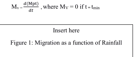
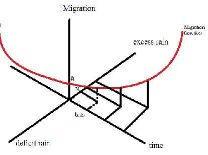
Migration Velocity Mv, is the rate at which the migration changes with respect to time. Note that
the time dimension in this model is having a specific definition, and it is the period when the Utility
is diminishing due to the πe or πd. Thus the migration velocity is the first derivative of the Monsoon
Migration function with respect to time beyond the tmin.
Mv = 𝑑(Mpt)𝑑𝑡 , where MV = 0 if t = tmin
This indicates that there will be no change in migration up to tmin. The Quantum of rain will be
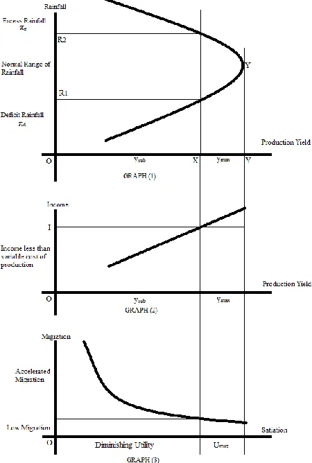
‘Normal Range’ during this period. In the figure (1), the normal range of rainfall is shown by N.
The utility will also be Umax up to the tmin. Beyond N, the rainfall is excess (πe). The Level Zero of
the Rainfall axis indicates the minimum rainfall of the Normal Range. If the rain fall is below this,
then there will be deficit rainfall (πd). During the tmin there may be a minimum migration which
[image:10.612.200.460.459.569.2]Insert here
11
could be caused due to other exogenous factors not included in the model. This is indicated by the
intercept of Migration axis of the Monsoon Migration function in the figure (1), which is ‘a’.
Beyond tmin±σt Migration Acceleration MA will set in. MA is the rate of change of Migration
Velocity with respect to time.
MA = 𝑑2(Mpt)
𝑑𝑡2 = 𝑑(Mv)
𝑑𝑡
It is observed in the Figure (1), that the migration function graph slope becomes steeper beyond
the tmin. As the time dimension increases the slope become steeper, and there is greater migration
velocity. The Migration velocity also changes continuously at an accelerated rate. This indicates
that the Migration Function is non-linear model. Only π with a tmin will decelerate the migration.
The Figure (2) has 3 graphs, graph (1), (2) and (3). The Graph (1) shows the relationship between
the rainfall range and the production yield. The Graph (2) shows the relationship between the
income and yield, and the graph (3) shows the relationship between the satiation (utility) and the
Migration.
The graph (1) in figure (2) indicates the relationship between the yield and the rainfall. It is like
the Laffer Curve. As shown, when the rainfall is in the Normal range π (R1 – R2 on y axis), the
yield is maximum (ymax) shown as XY on the x axis. If the rainfall enters the πe, that is rain fall is
more than OR2 then the yield reduces to ysub and this is shown by the OX on the x axis. Similarly,
if the rainfall enters the πd, that is rain fall is below OR1 then the yield reduces to ysub and this is
Inset here
12
shown by the OX on the x axis. Y is the maximum yield that can be produced at the most optimal
rainfall condition.
The graph (2) in figure (2) shows the production yield on the x axis and shows the changes in the
income level at each production level on the y axis. This graph also establishes the relationship
between the rainfall and the income of the cultivators. OI is the income level at which the minimum
variable cost of production is recovered and any income below this is a result of the ysub. The
optimum yield level generates income higher than the OI level.
The graph (3) in figure (2) shows Utility on the x axis and the quantum of migration on the y axis.
At ymax (higher yield) from graph (2), the satiation of the cultivator is maximum, i.e, Umax. (as
shown in graph 3).This will result inLow migration rates. The slope of the Utility curve is also
flat in this range showing that the migration velocity and acceleration is very low. When the ysub
occurs the utility diminishes and we can see that the utility curve starts to rise, indicating that the
migration is steadily increasing. At very low ysub levels the migration acceleration is very high and
the total migrated population increases exponentially.
From the discussion on figure (2), it can be established that the Mpt, the total migrated population,
is a function of the rainfall. Thus Monsoon Migration Model should, include time constraint tmin,
πe andπd elements. The excess or deficit rainfall is the quantitative aspect of the rainfall defined
based on the geographic cropping requirement. When migration from a specific location is being
quantified, it is required to record the actual rainfall in that geographic location and then check
whether the rainfall is ‘Normal’ or ‘Not Normal’ for that geographic cropping condition.
The monsoon migration model can be modelled as two equations below,
13
Mpt = β′1 + β2(R) + u ---- (equation 3)
In the above equations (2) and (3) Mpt= Number of families migrated in the year “t” × Number of
family members migrated. This means Mpt = Total Migration population in tth year. R = Actual
quantum of rain. While ‘u’ is the disturbance in the true model, which explains the deviations
caused by factors other than quantum of rainfall.
Equation 2 shows the total Migration under ‘Normal’ rain fall conditions and equation (3) shows
the migration under ‘Not Normal’ rainfall conditions.
Further let δ = β′1 - β1
The equation (2) and (3) are combined as Mpt = β1 + δ + β2(R) + u ---- (equation 4)
A dummy variable ‘NOT’ and a slope dummy variable ‘NOTR’ which is the product of ‘NOT’
and ‘R’ with ɣ as the coefficient is introduced in the equation (4). The dummy variable NOT can
take values of 1 or 0, where 1 indicates ‘Not Normal’ rainfall and 0 indicates ‘Normal’ rainfall.
The model considers the reference as ‘Normal’ rainfall. The equation (4) can be restated as below
Mpt = β1 + δ (NOT) + β2(R) + ɣ (NOTR) + u ---- (equation 5)
Mpt = β1 + δ (NOT) + (β2+ ɣ NOT) R + u ---- (equation 6)
Based on the theoretical framework of the Monsoon Migration model proposed, the equation (6)
can be simplified by stating that the migration percentage with respect to the population of the area
(%Mpt) is a function of the absolute deviation in the rainfall in percentage (%ADR).
That is (%Mpt)= f (%ADR).
Where, Percentage Migration (%Mpt) = (Actual Migration / Population of the Region) ×100
14
The following model is proposed.
ln(%Mpt) = β1 + β2 (%ADR) + u ---- (equation 6.a)
Hypothesis for the study
H0: There is no significant relationship between Percentage Migration (%Mpt) and Percentage
Absolute Deviation (%ADR)
Ha: There is a significant relationship between Percentage Migration (%Mpt) and Percentage
Absolute Deviation (%ADR)
Methodology
For the purpose of the empirical study, cross sectional data of the total migration from 28 states
and 7 union territories (UT) of India, as per the 2001 Census is considered (detailed enumerated
migration data of 2011 census is not yet published by the Government of India). For the same year,
2001, the rainfall statistics (Actual and Normal rainfall) for 36 rainfall zones/regions of India has
been considered (provided by National data centre of India Meteorological department). The
rainfall statistics from the rainfall zones were aggregated for each states and union territories. In
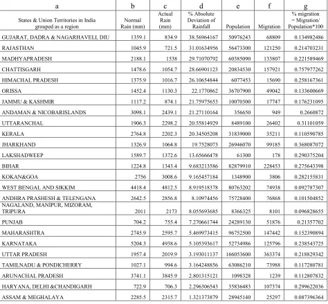
certain cases, the aggregation was done for more than one state and union territory. Table 1
provides the data of the Actual Rainfall (a), Normal rainfall (b), percentage of Absolute deviation
in rainfall (c), Population of the Zone (e) for different states and union territories in India.
In Table 1. for each rainfall zones (column a), the percentage deviation of actual rain (column c)
Insert here
15
from the normal rain (column b) is calculated and the absolute value of the same has been shown
in column d. Similarly, the percentage of migration (column g) with respect to the population
(column e) and actual migration (column f taken from the 2001 Census) has been shown. The
Census data for migration includes migrants for various purposes like education, work, marriage
and others. For the purpose of this study migration population is calculated by considering only
those who have migrated for the purpose of business or work/employment.
The proposed model considers states which are agriculturally sound. Analysis was carried out by
using rainfall statistics of 15 Indian states. Some states are not considered based on certain criteria.
Firstly, states (Arunachal Pradesh, Himachal Pradesh etc.) with low agricultural contribution to
state GDP are not considered. Some states like Jammu & Kashmir and Rajasthan are not
considered even though their agricultural contribution to the state GDP is high, because the type
of crop they grow (apples in J&K and mustard in Rajasthan), are rain independent. Urban States
like Goa and Delhi are not considered, as their contribution to agriculture is very minimal. Among
the seven eastern sister states, only Assam and Meghalaya are considered (Agricultural statistics
at a Glance).
Result of analysis
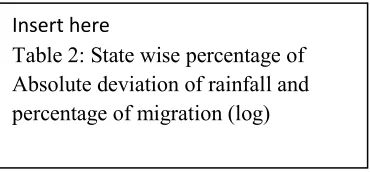
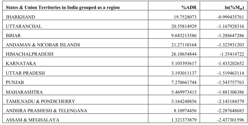
The equation (6.a) is tested empirically by fitting the regression using the data from Table 2.
The variables %ADR and ln(%Mpt) are taken as PERADEV and LNPERMIG respectively and
[image:15.612.214.399.594.680.2]Insert here
16
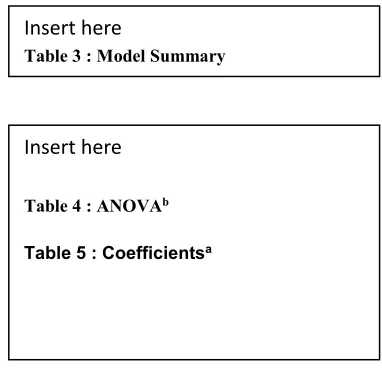
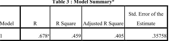
the LNPERMIG is regressed on PERADEV. The SPSS output for the Regression is as follows
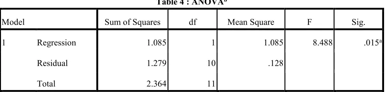
It is observed that the R2 from table 3, is 0.678 which indicates a good fit of the model, that is
67.8% of the dependent variable is predicted by the selected independent variables. The slope
coefficient of PERADEV from table 5 is 0.037 with a t-statistic of 2.913 which is significant. Thus
the null hypothesis H0 is rejected at 5% level of significance.
The equation (6.a) for this data can be written as follows,
ln(%Mpt) = -2.015 + 0. 037 (%ADR). ---- (equation 6.b)
Based on the regression output, the estimated “percentage of migration” against “the percentage
of absolute deviation in rainfall” is shown in figure 4.
[image:16.612.208.399.121.309.2]Insert here
Table 3 : Model Summary
Insert here
Table 4 : ANOVAb
Table 5 : Coefficientsa
Insert here
17
Equation 6(b) it follows that,
%Δ(%Mpt) ≈ (100×0.037) Δ (%ADR) --- (equation 6c)
Thus from equation (6c), it can be stated that one unit change in %ADR results in 3.7 percent
change in %Mpt
Enhancements to the Monsoon model in equation (6)
Based on the empirical study and continuing with the equation (6) restated below, the model can
be further enhanced to include the dummy variables for absolute deviation in rainfall and the
income variable.
Mpt = β1 + δ (NOT) + (β2+ ɣ NOT) R + u ---- (equation 6)
The ‘Not Normal’ rainfall condition can be either πe or πd and are introduced as dummy variables
with coefficients δe and δd respectively representing the change in migration due to the excess or
deficit rainfall. The πe or πd can take values of either 1 or 0.
If πe = 1, indicates excess rainfall and πd must be zero.
If πd = 1, indicates deficit rainfall and πe must be zero.
If both πe and πd = 0, indicates ‘Normal’ rainfall. Under any circumstances, it is not plausible for
both πe and πd to be equal to one.
Thus the equation (6) can be restated as below considering δe + δd = β′1 - β1
Insert here
Figure 4: Change in the Migration with Rainfall
18
Mpt = β1 + δe (πe) + δd (πd) + β2(R) + ɣe (πeR) + ɣd (πdR) +u ---- (equation 7)
From equation (7) the following equations results and can be used to quantify migration under
different rainfall conditions
Normal rainfall condition migration equation is Mpt = β1 + β2(R) +u
Excess rainfall condition migration equation is Mpt = β1 + δe πe + (β2+ɣe πe) R +u
Deficit rainfall condition migration equation is Mpt = β1 + δd πd + (β2+ɣd πd) R +u
The income status of the cultivator is also important for the migration (Deshingkar and Start,
2003). Middle income class and poor households with landholdings are more vulnerable to the
rainfall variations. A range of factors like limited alternative skills and small asset base can act
adversely in case of crop failure (Warner, Henry et.al, 2012). The very high income and low
income category of cultivators’ migrations are inelastic to ‘Not Normal’ rainfall range. The middle
income category cultivators’ migration is highly elastic to the ‘Not Normal’ rainfall.
Thus the migration model can also be defined based on income alone. Considering the need to
include a qualitative data of the income category of the cultivator, farmers household can be
classified into low income, middle income and high income category. The income is represented
as Y. As the middle income class migration is highly elastic to ‘Not Normal’ rainfall, middle
income category is considered as the base reference category for the model. H represents high
income category and L represents low income category and are taken as dummy variables in the
model. These dummy variables will have a value of 1 or 0, if the cultivator ‘belongs to’ or ‘does
not belong to’ the income category respectively. λH and λL are considered to be the slope
19
categories will be YH and YL. ξH and ξL are the incremental marginal change associated with
the high income and low income.
Thus the migration equation can be stated as a function of income alone as follows,
Mpt = β3 + λH (H) + λL (L) + β4(Y) + ξH (HY) + ξL (LY) +u ---- (equation 8)
Combining Equations (7) and (8), and taking βm= β1 + β3 the Income Monsoon Migration Model
is stated as below
Mpt= βm+δe(πe) +δd(πd) +β2(R) +ɣe(πeR) +ɣd(πdR) +λH(H) +λL(L) +β4(Y)+ξH(HY)+ ξL(LY)+u
---- (equation 9)
The Income Monsoon Migration model as proposed in equation (9) thus considers deficit and
excess rainfall to measure the migration. The proposed model is linear in parameter. The model
also considers the influence of income of the farmer household on migration. When H=0, the
model quantifies migration among low income category farmers. When L=0, migration among the
high income category cultivator can be estimated. For migration among the middle income
category cultivators, both H and L values are taken as 0.
Empirical study for the Income-Monsoon Migration Model
The empirical study for the Income monsoon migration model (equation 9) has not been conducted
because of the lack of availability of the relevant data. The model requires data specific to the
migrant population statistics from each rainfall zone, which also include their income before they
migrated. The rainfall data in India is being captured with respect to the rainfall zones. However,
this data need to be captured for specific cropping zones and the migration data captured by the
Census must also match the data for these cropping zones in order to empirically test the model.
20
Conclusion
A majority of employment generation in country like India is through the agriculture and allied
industries. Agriculture being predominantly dependent on the monsoon rains is vulnerable to
extreme climatic conditions. Farmers in rural areas mostly depend on agriculture for income. When
the income generated through this primary occupation is not sufficient, they are forced to migrate
to other areas, usually the urban locations. This intra-state and inter-state migration puts a lot of
pressure on the civic amenities in the urban destinations. Inadequate infrastructure and public
utility services puts a lot of stress on the existing facilities, thus reducing the welfare of the society
as a whole. Other adverse effects on wages in destination has also been widely studied and
documented. Therefore, a good estimation of the migration can provide sufficient data to the local
government to plan the infrastructure to support the incoming population and formulate policy
regulations necessary to increase the welfare of the society.
The monsoon migration model proposed and empirically tested in this paper will be able to
estimate the migration quantum from a specific geographic location based on the quantum of
rainfall. Further, this paper has also proposed the income-monsoon migration model which has an
additional variable, the income of the migrants from the specific location, for the estimation of
quantum of migration based on the migrant income. This model can be empirically tested provided
that the government of India collect enumeration data of the migrants specific to the cropping
zones with their income. This will enable to provide suggestions and insights to the government
21
References
Agricultural statistics at a Glance, Directorate of agriculture and statistics, http://eands.dacnet.nic.in/Advance_Estimate-2010.htm-
Barbieri, A.F., E. Domingues, B. L. Queiroz, R.M. Ruiz, J.I. Rigotti, J.A.M. Carvalho, and M.F. Resende (2010). Climate Change and Population Migration in Brazil’s Northeast: Scenarios for 2025-2050. Population and Environment, 31: 344-370.
Bardsley, DK; Hugo, GJ (2010). Migration and climate change: examining thresholds of change to guide effective adaptation decision-making. Population and Environment 32(2-3): 238-262
Bart W. Édes, François Gemenne, Jonathan Hill and Diana Reckien (2012). Addressing Climate Change and Migration in Asia and the Pacific. Asian Development Bank.
Black, R., D. Kniveton and K. Schmidt-Verkerk, (2011). Migration and Climate Change: Towards an Integrated Assessment of Sensitivity. Environment and Planning A, volume 43.
Byravan, S. and Rajan S.C (2009). Warming up to immigrants: An option for US climate policy. Economic and Political Weekly, 44, 19-23.
Dallman, I; Millock, K (2012). Climate variability and internal migration: a test on Indian inter-state migration. Paper Presented at the ENMRDTE Pre-conference on Migration and Environment, 17 October, 2012, Clermont-Ferrand, France
Datt G and M Ravallion (1998). Farm Productivity and rural poverty in India. Journal of Development Studies 34:4, 62-85
de Sherbinin, A., Warner, K., and Ehrhart, C. (2011). Casualties of climate change. Scientific American, 304(1), 64-71.
Deshingkar, P., and Start, D. (2003). Seasonal Migration for Livelihoods in India: Coping, Accumulation and Exclusion. Overseas Development Institute, London.
Dillon, A., V. Mueller, and S. Salau (2011). Migratory Responses to Agricultural Risks in Northern Nigeria. American Journal of Agricultural Economics, 93: 1048-1061.
22
Fernando Riosmena, Raphael J. Nawrotzki, Hunter Lori M, (2013). Rainfall Trends, Variability and U.S. Migration from Rural Mexico: Evidence from the 2010 Mexican Census Institute of Behavioral Science. Working paper
Gine, X., Townsend, R., and Vickery, J. (2008). Patterns of rainfall insurance participation in rural India. The World Bank Economic Review, 22(3), 539-566.
Gugler, J. (1988). Over Urbanization Reconsidered in J. Gugler (ed). The Urbanisation of the Third World. Oxford: Oxford University Press.
Hanmer, L., & Naschold, F. (2000). Attaining the International Development Targets: Will Growth Be Enough? Development Policy Review, 18(1), 11-36. doi: 10.1111/1467-7679.00098
Hassani-Mahmooei, B. and B.W. Parris (2012). Climate Change and Internal Migration Patterns in Bangladesh: An Agent-based Model. Environment and Development Economics, doi:10.1017/S1355770X12000290.
Hertel, T. W., and Rosch, S. D. (2010). Climate Change, Agriculture, and Poverty. [Article]. Applied Economic Perspectives and Policy, 32(3), 355-385.
International Organization for Migration (IOM), (2009). Migration, Environment and Climate Change: Assessing the evidence.
Kavi Kumar K. S. and Brinda Viswanathan, (2012). Weather variability and agriculture: implications for long and short-term migration in India. Center for Development Economics, Delhi school of Economics, Working paper No. 220
Kumar, KS Kavi; Parikh, J (2001). Socio-economic impacts of climate change on Indian agriculture. International Review of Environmental Strategies 2(2): 277-293
Lee ES, (1966). A Theory of Migration. Demography, 3(1), 47-57
Mall, RK; Singh, R; Gupta, A; Srinivasan, G; Rathore, LS (2006). Impact of climate change on Indian agriculture: a review, Climatic Change 78: 445-478
Marchiori, L., J-F. Maystadt, and I. Schumacher (2012). The Impact of Weather Anomalies on Migration in sub-Saharan Africa. Journal of Environmental Economics and Management, 63:355-374.
23
McLeman, R., and Hunter, L. M. (2010). Migration in the Context of Vulnerability and Adaptation to Climate Change: Insights from Analogues. Wiley Interdisciplinary Reviews: Climate Change, 1(3), 450-461.
McLeman, R; Smit, B (2006). Migration as an adaptation to climate change. Climatic Change 76(1-2): 31-53
Mellor, J. (1999). Faster, More Equitable Growth – The Relation Between Growth in Agriculture and Poverty Reduction Agricultural Policy Development Project (Research Report No. 4). Washington, D.C.: United States Agency for International.
Mitra Arup and Murayama Mayumi (2008). Rural to Urban Migration: A District Level Analysis for India. IDE Discussion Paper, No 137
Nawrotzki, RJ; Riosmena, F; Hunter, LM (2012). Do Rainfall Deficits Predict U.S.-Bound Migration from Rural Mexico? Evidence from the Mexican Census. Population Research Policy Review, doi: 10.1007/S11113-012-9251-8
Perch-Nielsen, S., Bättig, M., and Imboden, D. (2008). Exploring the link between climate change and migration. Climatic Change, 91(3-4), 375-393.
Perch-Nielsen, S; Battig, M; Imboden, D (2008). Exploring the link between climate change and migration. Climatic Change 91(3-4): 375-393
Ravenstein EG (1885). The Law of Migration. Journal of the Statistical Society of London, 48(2), 167-235
Sanchez Cohen, I., Oswald Spring, U., Diaz Padilla, G., Cerano Paredes, J., Inzunza Ibarra, M. A., Lopez Lopez, R., and Villanueva Diaz, J. (2012). Forced migration, climate change, mitigation and adaptation policies in Mexico: Some functional relationships. International Migration, 1-20, doi: 10.1111/j.1468-2435.2012.00743.x.
Schneider Kate and Gugerty Mary Kay (2011). Agricultural Productivity and Poverty Reduction: Linkages and Pathways, The Evans School Review, Vol. 1, Num. 1
Veena A and K Rao, Sandeep. (2017), Analysis of Socio Economic Conditions and Migration Patterns of Migrant Settlements in Bengaluru, Shinoda, Inoue and Suda (eds), Social Transformation and Cultural Change in South Asia: From the Perspectives of the Socio-Economic Periphery, ISBN 978-4-904626-27-6, (pp. 141-164), Tokyo: The Institute of Oriental Studies, Daito Bunka University.
24
Wang Chenggang, Rada Nicholas, Qin Lijian & Pan Suwen, (2014). Impacts of Migration on Household Production Choices: Evidence from China. The Journal of Development Studies, 2014 Vol. 50, No. 3, 413–425
Warner, K., Afifi, T., Henry, K., Rawe, T., Smith, C., de Sherbinin, A. (2012). Where the Rain Falls: Climate Change, Food and Livelihood Security, and Migration. Global Policy Report of the Where the Rain Falls Project. Bonn: CARE France and UNU-EHS.
25
26
27
Table 1. State wise Rainfall and Migration
a b c d e f g
States & Union Territories in India grouped as a region
Normal Rain (mm) Actual Rain (mm) % Absolute Deviation of
Rainfall Population Migration
% migration = Migration/ Population*100
GUJARAT, DADRA & NAGARHAVELI, DIU 1359.1 834.9 38.56964167 50976243 68809 0.134982486
RAJASTHAN 1045.9 721.5 31.01634956 56473300 121250 0.214703231
MADHYAPRADESH 2188.1 1538 29.71070792 60385090 133807 0.221589469
CHATTISGARH 1478.6 1054.7 28.66901123 20834530 157921 0.757977262
HIMACHAL PRADESH 1375.9 1016.7 26.10654844 6077453 15690 0.258167361
ORISSA 1452.4 1130.3 22.1770862 36707900 49042 0.133600669
JAMMU & KASHMIR 1117.2 874.1 21.75975653 10070300 17747 0.176231095
ANDAMAN & NICOBARISLANDS 3098.1 2439.1 21.27110164 356650 949 0.2660872
UTTARANCHAL 1906.3 2298.2 20.55814929 8489100 26402 0.31101059
KERALA 2764.8 2202.3 20.34505208 31839000 35211 0.110590785
JHARKHAND 1326.9 1064.8 19.7528073 26946070 99185 0.368087072
LAKSHADWEEP 1589.7 1372.6 13.65666478 61300 178 0.290375204
BIHAR 1224.8 1343.4 9.683213586 82879910 228453 0.275643398
KOKAN&GOA 2756 3008.6 9.165457184 1348900 3806 0.282155831
WEST BENGAL AND SIKKIM 4418.4 4812.5 8.919518378 80763202 74938 0.092787307
ANDHRA PRASHESH & TELENGANA 2642.5 2856.8 8.10974456 75728400 76868 0.101504852 NAGALAND, MANIPUR, MIZORAM,
TRIPURA 2011 2173 8.055693685 8366325 8101 0.096828655
PUNJAB 704.2 755.4 7.270661744 24289130 51876 0.21357702
MAHARASHTRA 2745.9 2595.7 5.469973415 96752500 147442 0.152390894
KARNATAKA 5204.3 4938.6 5.105393617 52734986 125796 0.238543725
UTTAR PRADESH 1957.4 2019.9 3.193011137 166053600 363374 0.218829342
TAMILNADU & PONDICHERRY 1027.1 994.6 3.164248856 63086210 73988 0.117280781
ARUNACHAL PRADESH 3741.1 3845.9 2.801315121 1098328 1239 0.112807832
HARYANA, DELHI &CHANDIGARH 722.9 706.3 2.296306543 35836483 107374 0.299622036
28
Table 2: State wise percentage of Absolute deviation of rainfall and percentage of migration (log)
States & Union Territories in India grouped as a region %ADR ln(%Mpt)
JHARKHAND 19.7528073 -0.999435761
UTTARANCHAL 20.55814929 -1.167928316
BIHAR 9.683213586 -1.288647286
ANDAMAN & NICOBAR ISLANDS 21.27110164 -1.323931203
HIMACHALPRADESH 26.10654844 -1.35414722
KARNATAKA 5.105393617 -1.433202652
UTTAR PRADESH 3.193011137 -1.519463114
PUNJAB 7.270661744 -1.543757763
MAHARASHTRA 5.469973415 -1.881306386
TAMILNADU & PONDICHERRY 3.164248856 -2.143184379
ANDHRA PRASHESH & TELENGANA 8.10974456 -2.287648683
29
Table 3 : Model Summaryb
Model R R Square Adjusted R Square
Std. Error of the Estimate
1 .678a .459 .405 .35758
a. Predictors: (Constant), PERADEV
30
Table 4 : ANOVAb
Model Sum of Squares df Mean Square F Sig.
1 Regression 1.085 1 1.085 8.488 .015a
Residual 1.279 10 .128
Total 2.364 11
a. Predictors: (Constant), PERADEV
31
Table 5 : Coefficientsa
Model
Unstandardized Coefficients
Standardized Coefficients
t Sig.
B Std. Error Beta
1 (Constant) -2.015 .172 -11.726 .000
PERADEV .037 .013 .678 2.913 .015
32
33