Cyclicality and Firm-size in Private Firm Defaults

City, University of London Institutional Repository

Citation

: Jensen, T., Lando, D. & Medhat, M. (2017). Cyclicality and Firm-size in Private

Firm Defaults. International Journal of Central Banking(Dec),

This is the accepted version of the paper.

This version of the publication may differ from the final published

version.

Permanent repository link:

Link to published version

:

Copyright and reuse:

City Research Online aims to make research

outputs of City, University of London available to a wider audience.

Copyright and Moral Rights remain with the author(s) and/or copyright

holders. URLs from City Research Online may be freely distributed and

linked to.

Cyclicality and Firm-size in

Private Firm Defaults

Thais Lærkholm Jensen,

David Lando,

Mamdouh Medhat

This version: July 8, 2016

Abstract

The Basel II/III and CRD-IV Accords reduce capital charges on bank loans to smaller firms by assuming that the default probabilities of smaller firms are less sensitive to macroeconomic

cycles. We test this assumption in a default intensity framework using a large sample of bank

loans to private Danish firms. We find that controlling only for size, the default probabilities

of small firms are, in fact, less cyclical than the default probabilities of large firms. However,

accounting for firm characteristics other than size, we find that the default probabilities of

small firms are equally cyclical or even more cyclical than the default probabilities of large

firms. These results hold using a multiplicative Cox model as well as an additive Aalen model

with time-varying coefficients.

Keywords: Capital charges·SME·Default risk·Macroeconomic cycles

JEL: G21, G28, G33, C41

∗_{Lærkholm Jensen is at Department of Economics, University of Copenhagen, and the Danish Central Bank.}

Lando is at Department of Finance and FRIC Center for Financial Frictions, Copenhagen Business School. Med-hat is at Faculty of Finance, Cass Business School, City University London. Send correspondence to David Lando,

dl.fi@cbs.dk,+45 3815 3613, Solbjerg Plads 3, DK-2000, Frederiksberg, Denmark.

1

Introduction

Small and medium-sized enterprises (SMEs) typically depend more heavily on funding from banks

than do larger firms. It is therefore conceivable that SMEs are hit harder during a financial crisis

in which banks’ capital constraints are binding. As a way to facilitate bank funding of SMEs, the

Basel II Accord prescribes lower capital charges for loans to the SME-segment. Technically, the

reduction in capital charges is implemented by prescribing a lower asset correlation to be used

when calculating capital charges. To the extent that asset correlation arises because of common

dependence on macroeconomic shocks, the reduction corresponds to assuming that the default

probabilities of SMEs are less sensitive to macroeconomic cycles than those of larger firms. These

reductions in capital charges were recently reaffirmed and extended in the Basel III Accord and in

the fourth Capital Requirements Directive (CRD-IV).1

This paper uses a large sample of loans to private Danish firms to test whether there is empirical

support for the assumption that the default probabilities of smaller firms are less cyclical. Our

results indicate that solely discriminating with respect to firm-size, the default probabilities of

small firms are in fact less sensitive to macroeconomic cycles compared to the default probabilities

of large firms. However, when we account for differences in firm-characteristics other than size, our

results indicate that the default probabilities of small firms are as cyclical or even more cyclical

than the default probabilities of large firms. This indicates that the size effect arises because of

omitted variables. These results are robust to different regression models and different ways of

dividing our sample into small and large firms. The evidence form our data suggests that a bank

that properly accounts for firm characteristics in its default risk modeling will not experience a

weaker effect of economic cycles in the SME segmemt, and hence the reduced capital charge will

in fact make a bank with a high exposure to the SME-segment more risky.

According to theEuropean Commission’s (2016) annual report, SMEs comprised over 99% of

all enterprises, accounted for 67% of total employment, and stood for over 70% of job growth in the

non-financial business sector in the 28 EU countries. Hence their importance for the economy

pro-vides a political justification for the separate treatment. Furthermore, shifting banks’ risk-exposure towards smaller firms could be in the interest of regulators—for instance because larger firms are

more likely to have larger loans or loans across several banks, which could create contagion within

and across banks in case of defaults. But such effects are already accounted for using so-called

1_{Article 273 ofThe Basel Committee on Banking Supervision’s (2006) report states the following: “Under the}

IRB approach for corporate credits, banks will be permitted to separately distinguish exposures to SME borrowers (defined as corporate exposures where the reported sales for the consolidated group of which the firm is a part is less thane50 million) from those to large firms. A firm-size adjustment [...] is made to the corporate risk weight formula for exposures to SME borrowers.”

‘granularity adjustments’. Our focus is on whether an additional adjustment of capital charges

through lower correlation with the macroeconomic environment can be justified empirically.

Our data covers the period 2003-2012 and consists of obligor, loan, and default information for

a large sample of private Danish firms. We devise two different ways of testing whether defaults

of smaller firms are more or less cyclical. First, we use the standard multiplicative Cox regression

model to estimate the effects of firm-specific and macroeconomic variables on default intensities.

Our Cox models confirm previous findings that accounting ratios and macroeconomic variables

play distinct roles in default prediction for private firms: (1) Accounting ratios are necessary for

accurately ranking private firms according to default likelihood, but cannot by themselves capture

the cyclicality of aggregate default rates, while (2) macroeconomic variables are indispensable for

capturing the cyclicality of aggregate default rates, but do not aid in the ranking of firms with

respect to default likelihood. Using our fitted Cox model, we find that when we split our sample

with respect to firm size and keep all other firm characteristics fixed, the default probabilities of smaller firms do in fact exhibit less sensitivity to macroeconomic cycles. This is in the sense

that the effects of macroeconomic variables are generally of smaller magnitude for smaller firms.

However, when we account for the Cox model’s non-linear form and use averaging techniques

adapted from other non-linear regression models, our results indicate that the default probability

of the average small firm may be as cyclical or even more cyclical than the default probability of

the average large firm.

Second, we investigate our data using the more flexible additive Aalen regression model. The

additive model allows us to estimate time-varying effects of firm-specific variables, which is a

potentially important component of the cyclicality of default probabilities that is missing from our

Cox model. Furthermore, due to the linearity of its effects, the additive model allows us to directly

compare the effects of macroeconomic variables for small and large firms without the need for

averaging techniques. Our analysis based on the additive model reveals, in particular, that firm-size

has a significantly time-varying and mostly negative effect. Hence, the effect of firm-size varies

significantly the with business-cycle but is generally such that that larger firms have lower default

probabilities. Moreover, the effect of firm-size reaches its largest (negative) magnitude during the

financial crisis of ‘08-‘10, which indicates that larger firms were safer, not riskier, during the most

recent recession. Lastly, using our fitted additive model and splitting the sample with respect to firm

size, we again find no evidence that there is a difference in the signs, magnitudes, or significance of

the effects of our macroeconomic variables for small firms compared to large firms. These results

indicate that our main findings are robust to different regression models that capture cyclicality in

Our results indicate that a different treatment of capital charges solely based on firm-size is too

simplistic, as it ignores other important characteristics that differ between small and large firms.

This suggests that imposing solely size-based preferential treatment of capital charges may, in fact,

increase the risks of banks with a high exposure to the SME-segment.

The outline of of the paper is as follows. Section 2 explains the piece of the Basel regulation

that motivates our study. Section 3 reviews the literature. Section 4 details our data and variable

se-lection. Section 5 provides our estimation methodology. Section 6 presents our regression results

for identifying the firm-specific and macroeconomic variables that significantly predict defaults.

Section 6 presents our results regarding the sensitivity of small and large firms’ default

probabili-ties to macroeconomic variables. Section 7 shows results related to robustness and model check.

Section 8 concludes.

2

The Basel capital charge for loans

Basel II and III allow banks to estimate capital requirements for small and medium-sized

corpo-rations (SMEs) using a risk weight formula that includes a lower asset correlation with

macroe-conomic risk-drivers compared to that of larger corporations. The exact formulation in Basel II

can be found in Articles 273 and 274 of The Basel Committee on Banking Supervision’s (2006)

report. The same provisions are carried forward and extended in the Basel III Accord and the

re-cently adopted CRD-IV as Articles 153.4 and 501.1 ofThe European Parliament and the Council

of the European Union’s (2013) report.

The amount of equity capital required for funding a loan essentially depends on the unexpected

loss (UL) per unit principal,

UL=LGD(θ∗−PD),

where PD is the loan’s one-year probability of default, LGD is the loss rate given default, and

θ∗_{= Φ}

      

1 p

1−ρ

Φ−1

(PD)+ √ρΦ−1(0.999)

     

. (1)

Here, Φ is the standard normal distribution function and θ∗ is the 99.9% worst case default rate.

The correlation parameter,ρ, that goes into this calculation is PD-dependent and prescribed by the

Basel documentation (after removing the negligible terms exp(−50)) as

ρ(PD)=0.12 1−exp(−50 PD)+0.24 exp(₋50 PD).

For SMEs with annual sales,S, up toe50 million, this correlation is modified to

ρ(PD)=0.12 1−exp(−50 PD)+0.24 exp(₋

50 PD)−0.04 1− max(S −5; 0)

45 !

,

where the last term has the effect of lowering the capital requirement. The exact capital requirement

depends on the contribution to Risk Weighted Assets (RWA), which depends on UL, the

Exposure-at-Default (EAD), and a maturity adjustment whose exact form need not concern us here.

As an illustration of the economic magnitude of the reduction in capital requirement for SMEs,

note that with an annual default probability of 1%, a loan to an SME withS =e25 million achieves

a deduction in asset correlation of 11.52% relative to an equally risky non-SME. Assuming an LGD

of 15% and an effective maturity of 2.5 years (both provided as “representative averages” by the

financial institution that provided us with the data), we calculate that this corresponds to deduction

of 12.14% in capital requirement.

In the derivation of the capital charge formula,ρrepresents correlation between asset values of

different borrowers which arises because the asset values depend on a common economy-wide

fac-tor. Therefore, the reduction in correlation for SMEs corresponds to an assumption that these firms

have default probabilities that are less sensitive to the economy-wide factor. It is this assumption

that we will devise two ways of testing on a large Danish data set.

3

Related literature

There is conflicting evidence in the literature regarding the validity of the assumption in the Basel

Accords that the default probabilities of smaller firms are less cyclical. Lopez (2004) employs

the KMV approach on a sample of US, Japanese, and European firms and finds that average asset

correlation is a decreasing function of probability of default and an increasing function of

firm-size, which is line with the assumption in the Basel Accords. Dietsch and Petey(2004), however,

use a one-factor credit risk model on a sample of French and German firms and find that SMEs

have higher default risk than larger firms and that the asset correlations for SMEs are weak and

decrease with firm-size. Chionsini, Marcucci, and Quagliariello (2010) use firm-size dependent

firms and they find support for the size-dependent treatment in the Basel Accord, though not during

severe financial crises like that of 2008-09. Jacobson, Linde, and Roszbach (2005) use a

Monte-Carlo resampling method for a sample of Swedish firms and find little support for the hypothesis

that SME loan portfolios are less risky, or require less economic capital, than corporate loans.

Our approach differs from these studies in that we use an intensity regression framework to

directly estimate and study how default probabilities simultaneously depend on a large set of

firm-characteristics, including size, as well as macroeconomic variables. This allows us to determine

the firm-characteristics that are important for accurately ranking firms with respect to default

like-lihood as well as the macroeconomic variables important for capturing the cyclicality of default

rates over time. Importantly, our approach has the advantage of allowing us to directly

deter-mine how the effects of macroeconomic variables on default probabilities differ for small and large

firms while simultaneously controlling for firm-characteristics other than size. We apply averaging

techniques to the Cox regression model resembling those commonly applied to generalized linear

models—see, for instance,Wooldridge(2009, p. 582-83) for an overview. The additive regression

model due toAalen(1980, 1989), was applied in a default prediction setting byLando, Medhat,

Nielsen, and Nielsen (2013). They show that there is significant time-variation in how certain firm-specific variables influence the default probabilities of public US firms.

Statistical models using accounting ratios to estimate default probabilities date back to at least

Beaver (1966) and Altman (1968), followed by Ohlsen (1980) and Zmijewski (1984)—we use

many of the same accounting ratios as in these studies. Shumway(2001) was among the first to

demonstrate the advantages of intensity models with time-varying covariates compared to

tradi-tional discriminant analysis, and was also among the first to include equity return as a market-based predictor of default probabilities—we use a similar estimation setup, although we do not

have market-based variables for our private firms. Chava and Jarrow(2004) improved the setup

ofShumway(2001) using covariates measured at the monthly level and showed the importance of

industry effects—our data frequency is also at the monthly level and we correct for industry effects

in all our regressions.

Structural models of credit risk, like the models ofBlack and Scholes (1973), Merton(1974),

andLeland (1994), usually assume that a firm defaults when its assets drop to a sufficiently low level relative to its liabilities. The connection between structural models and intensity models was

formally established by Duffie and Lando (2001), who showed that when the firm’s asset value

process is not perfectly observable, a firm’s default time has a default intensity that depends on the

firm’s observable characteristics as well as other covariates. Studies demonstrating the importance

of covariates implied from structural models, like distance-to-default or asset volatility, include

Probability of default and the macroeconomy Thais Lærkholm Jensen

Page | 42

bank recorded the first interaction with the client. Entry year specifies the year at which the firm enters the sample while duration is the number of years a firm is observed in the sample since its entry year.

From the onset of the analysis a larger stock of firms exist in the sample in 2003 and an inflow of new firms to the sample happens in the following years. Figure 6 (a) shows the numbers of firms entering the sample each year. Despite discussions with Danske Bank, the low number of firms entering the sample in 2005 cannot be explained. It appears however, by the black line, that the firms that eventually default do not seems to differ systematically from the non-defaulting firms based on when they enter the sample. While the 2005 entry levels remains a conundrum, the similarity in default and non-defaulting firms’ entry patterns is taken to imply that the independent censoring assumption is not violated based on entry year.

Figure 6: Examining entry year and risk set

(a) (b)

Figure 6 (b) shows on the left vertical axis, the risk set which is the number of firms which are observed in a given quarter and therefore potentially at risk of default. On the right hand side is the quarterly number of defaults. As firms continuously enter and leave the data-set the sample size varies over time. What is remarkable is the approximately 2000 firm drop in the risk set from 2004 to 2005 which cannot be explained by the only 22 defaults in 2004:Q4. A large number of firms are simply lost to follow-up, while, as noted, very few firms enter the sample this year.

0 20 40 60 80 100 120 140 160

0 500 1000 1500 2000 2500 3000

Number

of

entries

Entry of Firms (LHS) Entry of Non Defaults (LHS) Entry of Defaulting (RHS)

0 10 20 30 40 50 60 70

0 1000 2000 3000 4000 5000 6000 7000 8000 9000

Quarly

number

of

defaults

Number

of

firms

in

risk

set

Firms in Risk Set (LHS) Firms Defaulting (RHS)

Notes: Figure 6 (a) shows yearly number of entering firms based categorized by firm eventually default or non-default. Figure 6 (b) shows the quarterly number of observed defaults in the sample along with the number of firms in the risk set

Figure 1. Entry and at-risk pattern in the sample. The left panel shows the yearly number of firms entering the sample (grey mass) along with the yearly number of entries that do not default (black, solid line) or eventually do default (black, dashed line). The right panel shows the quarterly number of firms at risk of defaulting (i.e. in the “risk set”; grey mass) along with the actual number of defaulting firms in each quarter (black, solid line).

Duffie, Saita, and Wang (2007), Bharath and Shumway (2008), Lando and Nielsen (2010), and

Chava, Stefanescu, and Turnbull(2011) among many others.

Default studies using data on public firms and demonstrating the importance of employing

macroeconomic variables includeMcDonald and de Gucht (1999), Peseran, Schuermann,

Treut-ler, and Weiner (2006),Duffie et al.(2007), Lando and Nielsen(2010),Figlewski, Frydman, and Liang(2012), among many others. Recent default studies of private firms that also employ

macroe-conomic variables includeCarling, Jacobson, Lind´e, and Roszbach(2007), who use Swedish data,

and Bonfim (2009), who uses Portuguese data. We employ many of the same macroeconomic variables as in these studies.

4

Data and variables

This section presents our data and the variables that we employ as firm-specific and

macroeco-nomic drivers of default probabilities.

Our raw data comprises 28,395 firms and 114,409 firm-year observations of obligor and loan

histories, accounting statements, and default indicators over the period 2003 to 2012. The data

is obtained from a large Danish A-IRB (advanced internal ratings-based approach) financial

insti-tution. A firm is included in this dataset if it has an engagement over DKK 2 million in at least

one of the years underlying the period of analysis. An engagement is defined in terms of loans or

granted credit lines. After removing sole proprietorships, government institutions, holding

0.0% 0.1% 0.2% 0.3% 0.4% 0.5% 0.6% 0.7% 0.8% 0.9%

0 200 400 600 800 1000 1200 1400 1600 1800

0.0% 0.5% 1.0% 1.5% 2.0% 2.5% 3.0%

0 1000 2000 3000 4000 5000 6000 7000

Aggregate number of bankruptcies (LHS) Aggregate number of bankruptcies (LHS)

Default rate within our sample (RHS) Default rate within our sample (RHS)

Figure 2. Default rates in the sample and the general Danish economy.The left panel shows the quarterly default rate from the sample along with the corresponding aggregate number of quarterly bankruptcies in the general Danish economy. The right panel shows the yearly default rate from the sample along with the aggregate quarterly number of default in the general Danish economy.

and firms with insufficient balance sheet information, we are left with 10,671 firms and 48,703

firm-year observations. In the cleaned dataset, a total of 633 firms experienced a default event, defined by the Basel II Accord as more than 90 days delinquency. Moreover, 54 of the 633

de-faulting firms experience a second default, in the sense that they became delinquent a second time

during the sample period. Other default studies have treated a firm that re-emerges from default as

a new firm. In accordance with the Basel II Accord’s definition of a default event as a period of

delinquency, we choose to disregard multiple default events, so that only the initial default counts.

Figure 1shows the patterns by which firms enter and potentially leave our final sample. The

right panel shows the number of firms that enter the sample at each year along with an indication of

the number of entries eventually corresponding to defaults and non-defaults. Despite discussions

with the financial institution providing the data, the low number of firms entering the sample in 2005 remains a conundrum. It appears, however, that the firms that eventually default do not seem

to differ systematically from the non-defaulting firms based on when they enter the sample. The

right panel shows the number of firms at risk of defaulting, i.e. firms in the “risk set,” at each

quarter, along with the quarterly number of defaults. The risk set is seen to contain at least 2,000

firms at each quarter, and the 2008-09 financial crisis is readily visible from the sharp rise in the

number of defaults.

In order to incorporate quarterly macroeconomic variables, we re-code the accounting variables

for each firm from annual to quarterly observations. This will naturally induce persistence in

the accounting variables from quarter to quarter, which we correct for by basing all inference on

standard errors clustered at the firm-level. The final dataset thus consists of a total of 192,196

firm-quarter observations.

Figure2compares the observed default rate in our sample to the number of registered

bankrupt-cies in Denmark. The comparison is feasible because the total number of firms at risk of default in Denmark is relatively stable over time. We see that, due to the relatively few incidences, the

default rate in the sample co-moves nicely with the aggregate level in Denmark. This indicates that

our results are not likely to be representative for all Danish SMEs.

4.1

Firm-specific explanatory variables

Table 1provides an overview of the firm-specific explanatory variables which we employ in our

regression analysis. Our firm-specific explanatory variables measure size, age, leverage,

profitabil-ity, asset liquidprofitabil-ity, collateralization, and (book) equity. The table also gives the accounting ratios which we use to proxy for the firm-specific explanatory variables along with the expected sign of

each accounting-based variable’s effect on default probabilities. All our accounting-based

vari-ables have been applied in previous default studies, and the expected signs of their effects are both

intuitive and well-discussed in the literature—see, for instance,Ohlsen(1980),Shumway(2001),

Duffie et al.(2007), andLando and Nielsen(2010). We also correct for industry effects as inChava and Jarrow (2004). The main difference between our list of firm-specific variables and the ones used in default studies of public firms is the lack of market-based measures like stock return and

distance-to-default.

We control for industry effects since certain industry characteristics may prescribe a certain

leverage structure, for example because of differences in the volatility of cash flows. We use the

sector affiliation by Statistics Denmark to identify a firm’s primary industry as either

“Construc-tion,” “Manufacturing,” or “Wholesale and Retail,” as these have above average default rates, but

are at the same time coarse enough to ensure a sufficient number of firms in each sector.

Table2presents summary statistics for our firm-specific explanatory variables. An analysis of

the variables revealed a few miscodings and extreme values. Due to the anonymized nature of the

data, we were not able to check the validity of these data points manually, and we therefore choose

to winsorize all the firm-specific variables at the 1st and 99th percentile—a practice also used by

Chava and Jarrow(2004),Shumway(2001), andBonfim(2009), among others. The average firm has DKK 275 million in assets, a total debt to total assets ratio of 68%, and interest payments

corresponding to 3% of total assets. Further, the average firm had a relationship with the bank for

23 years and remains in the sample for 7 out of the 9 years.

rev-Table 1. Firm-specific explanatory variables and corresponding, observable accounting-based variables. The left column shows our list of firm-specific explanatory variables, the center column shows the observable accounting-based variables which we use as proxies, and the right column shows the expected effect of each accounting-based variables on default probabilities. Industry Effects are included in the list for completeness, although we only use this variable as a control (see details in the text).

Probability of default and the macroeconomy Thais Lærkholm Jensen

Page | 15

2.1

Internal explanatory variables

Due to the rich data set provided by Danske Bank, a number of firm specific accountancy variables have been investigated. While macroeconomic variables may facilitate a good view of the aggregate level of defaults in an economy, it is ultimately the financial situation of a firm that is determining whether or not a firm becomes delinquent. The microstructure also facilities a deeper understanding of which segments within a sample that are particularly affected by the macroeconomic variables. Also, it enables the credit institution to perform an ordinal ranking and assess which firms are more likely to default.

Table 2 provides an overview of internal explanatory variables that will be examined in turn below. In addition to the explanatory variables, the measurement used to capture the variables is also listed along with the expected effect on the probability of default. Sources and definitions of the measurements are given in Appendix 1.

Table 2: Internal variables and their expected effect on default probability

Explanatory Variable Investigated Measurements Expected effect on probability of default

Size _{Log of book value of assets Negative}

Age Years active in the bank Negative

Leverage

Short term debt to total assets Positive

Total debt to total assets Positive

Interest bearing debt to total assets Positive

Interest payments to total assets Positive

Profitability

Net income to total assets Negative

EBIT to total assets Negative

EBITDA to total assets Negative

Liquidity Current ratio Negative

Quick ratio Negative

Collateralization Fixed assets to total assets Negative

PPE to total assets Negative

Negative equity Dummy for negative equity Positive

Industry Effects DB07 Sector affiliation Control variable

Notes: Sources and definitions of measurements are given in appendix 1. All variables are in the estimation lagged one year to allow for prediction of default.

Proxy

enue and employee count, and hence these variables are zero (or missing) for a large proportion of

firms in the sample. We therefore choose not to use these two variables in our further analysis in

order to retain a large sample of smaller firms. In Table 2, firm age is taken to be time since the

bank recorded the first interaction with the client, entry year specifies the year at which the firm enters the sample, and duration is the number of years a firm is observed in the sample since its

entry year. The negative (book) equity dummy has an unconditional mean of 0.063, meaning that

just over 6% of our firm-quarters show a negative value of (book) equity.

4.2

Macroeconomic explanatory variables

Table 3 provides an overview of the macroeconomic explanatory variables which we employ in

our regression analysis. Our macroeconomic explanatory variables cover the stock market, interest

rates, GDP, credit supply, inflation, industrial production, as well as demand for consumer goods. The table also gives the observable time-series which we use to proxy for the macroeconomic

explanatory variables along with the expected sign of each time-serie’s effect on default

Table 2. Descriptive statistics for the firm-specific variables. The table shows descriptive statistics for the firm-specific variables of the cleaned sample, winsorized at the 1stand 99th percentile. The total number of observations is 192,196 firm-quaters. Age is time since the bank recorded the first interaction with the client. Entry is the year where the firm entered the sample. Duration is the number of years the firm remains in the sample. All other variable have standard interpretations.

Probability of default and the macroeconomy Thais Lærkholm Jensen

Page | 41

percentiale recpectively. Unfortunately the data from Danske Bank includes miscodings14 and due

to the anonymization of the data it has been infeasible to check any of these recordings manually.

As a result, the approach taken here has also been to winsorize the data at the 1st and 99th percentile.

The winsororized summary statistics are presented in Table 6 while Appendix 8 presents summary

statitistics by default status.15

The average firm has DKK 275 million assets, a ratio of 68% between total debt to total assets and interest payments corresponding to 3% of total assets. Furthermore the average firm had a relationship with the bank for 23 years and remains in the sample for 7 out of the 9 years.

Table 6: Summary statistics for the cleaned data

Variable Mean Std 1% 5% 25% 50% 75% 95% 99%

Total assets (tDKK) 275.074 1.060.373 811 2.784 9.553 28.222 100.723 1.025.875 8.656.000

Revenue (tDKK) 242.031 885.431 0 0 0 0 70.925 1.097.486 6.733.409

Employees 113 348 0 0 1 18 64 484 2.666

Age (years) 23 20 1 3 9 18 30 71 97,25

Log(total assets) (tDKK) 10,46 1,81 6,70 7,93 9,16 10,25 11,52 13,84 15,97 Short term debt to total assets 0,51 0,28 0,01 0,09 0,30 0,49 0,69 0,96 1,58 Total debt to total assets 0,68 0,28 0,02 0,18 0,53 0,70 0,84 1,04 1,80 Interestbearing debt to total assets 0,39 0,28 0,00 0,00 0,17 0,37 0,56 0,87 1,38 Interest payments to total assets 0,03 0,03 0,00 0,00 0,01 0,02 0,03 0,07 0,17

Current ratio 1,66 2,42 0,03 0,28 0,88 1,17 1,59 3,80 20,21

Quick ratio 1,28 2,37 0,02 0,14 0,49 0,81 1,19 3,15 19,67

Fixed assets to total assets 0,40 0,29 0,00 0,01 0,14 0,36 0,63 0,93 0,99 Tangible Assets to total assets 0,30 0,28 0,00 0,00 0,06 0,23 0,49 0,87 0,97 Net Income to total assets 0,03 0,14 -0,68 -0,18 0,00 0,03 0,09 0,24 0,43

EBIT to total assets 0,06 0,15 -0,59 -0,16 0,00 0,05 0,12 0,29 0,51

EBITDA to total assets 0,10 0,15 -0,51 -0,12 0,02 0,09 0,17 0,34 0,54

Entry Year 2005 1,94 2003 2003 2003 2004 2006 2009 2010

Duration (Years) 7 2 1 2 5 7 9 9 9

Notes: Table shows descriptive statistics for the cleaned sample winsorized at the 1st _{and 99}th _{percentile with 192.196 observations}

in total. Age is taken to be time since the bank recorded the first interaction with the client. Entry is the year when the firm entered the sample. Duration is how many years the firm remains in the sample. All other variable have standard interpretation and are further described in Appendix 1.

As shown in Table 6, revenue and employee count takes the value zero for a large proportion of observations. This is due to Danish reporting standards that allow firms below a certain size to refrain from reporting these numbers. As a result, these two variables are not used for further analysis in order not to discriminate against the smaller firms. Age is taken to be time since the

14 _{E.g. one firm was recorded as having 1.3 million employees while the largets company in Denmark employs only}

approximately 0.1 million employees.

15 _{Appendix 8 also presents summary statistics for the group of firms that leave the sample for other reasons that default.}

ities. The macroeconomic time-series are primarily obtained from Ecowin, with additional data

from Statistics Denmark, OECD, and Stoxx.

The inclusion of lagged macroeconomic variables allows us to use these to compute growth

rates, differences, or levels. We select the appropriate form by 1) computing the correlation

be-tween each form of the macroeconomic variable and the observed default rate, and 2) visually

inspecting the relationship of each form with the observed default rate. Note, however, that some pairs of the macroeconomic variables exhibit collinearity—for example, the Danish GDP growth

and the European GDP growth rate, as well as the return on the OMX index and the Stoxx index,

have pair-wise correlations of 0,92 and 0,77, respectively. The high degree of collinearity should

Table 3. Macroeconomic explanatory variables and corresponding observable time-series.The left column shows our list of macroeconomic explanatory variables, the center column shows the macroeconomic time-series which we use to measure each macroeconomic explanatory variable, and the right column shows the expected effect of each macroeconomic time-series on default probabilities.

Probability of default and the macroeconomy Thais Lærkholm Jensen

Page | 23

wide range of models examined. Duffie et al. (2007) surprisingly finds that default intensities

increase when the trailing one-year return of S&P 500 increases. The explanation given is that this might be due to the mean reverting nature of business-cycles.

Table 4: External variables and their expected effect on default probability

Explanatory Variable Investigated Measurements Expected effect on probability of default

Stock return Return of OMX index Negative

Stock volatility Volatility of OMX index Unknown Interest rates Slope of yield curve Negative

GDP Real growth in Danish GDP Negative

Loan growth Loan growth to non-financial firms Positive

Credit availability Funding costs Positive

Aggregate defaults Danish bankruptcies Positive

Inflation Headline CPI Unknown

Demand side effects Consumer confidence Negative

House prices Negative

Supply side effects Business indicator, manufacturing Negative Capacity utilization Negative

International exposure

Exports to Danish GDP Unknown Return of Stoxx50 index Negative

EU 27 GDP growth Negative

Notes: Sources and definitions of macroeconomic variables are given in Appendix 2. All variables are in the estimation lagged one year to allow for prediction of default.

The volatility of equity indices may signal the unrest in the economy, and as consequently higher volatility would be expected to be positively correlated with default rates. This is also the argumentation of Figlewski, et. al (2012) in their analysis, although their volatility measure ultimately turns out to be an insignificant predictor of default. On the other hand, studying models of endogenous defaults, Lando (2004) argues that increasing volatility may also lower the optimal default point, making defaults less likely to occur for troubled firms. This discrepancy makes the expected effect of volatility unknown.

The most liquid and closely monitored index in Denmark is the OMX index and is consequently adopted for calculating equity volatility and stock returns. One caveat to using the OMX equity index for Denmark is however that this index only includes the largest and perhaps most resilient firms in Denmark, and consequently might not be adequately capturing how smaller firms are impacted by the business cycle.

Proxy

5

Estimation methodology

This section present the methodology which we apply to estimate the effects of our explanatory

variables on firm-specific default probabilities.

Suppose we have a sample of nlevered firms observed over a time-horizon [0,T], where firm

imay default at a stochastic time τi. At each time t, the firm’s financial state is determined by a

vectorXit of firm-specific variables and by a vector Zt of macroeconomic variables, with values

common to all firms in the sample. Default at timetoccurs with intensityλit= λ(Xit,Zt), meaning

thatλitis the conditional mean arrival rate of default for firm i, measured in events per time unit.

Intuitively, this means that, given survival and the observed covariate histories up to timet, firm

i defaults in the short time-interval [t,t + dt) with probability λitdt.2 We assume τi is

doubly-stochastic driven by the combined history of the internal and external covariates (see for instance

Duffie et al.,2007).

We devise two different ways of testing whether defaults of smaller firms are more or less

2_{Precisely, a martingale is defined by 1} (τi≤t)−

Rt

01(τi>s)λisdswith respect to the filtration generated by the event

(τi>t) and the combined history of the firm-specific and macroeconomic variables up to timet.

cyclical. First, we use the standard multiplicative Cox regression model to estimate the effects of

firm-specific and macroeconomic variables on default intensities. Second, we use the more flexible

additive Aalen regression model which allows for time-varying effects of firm-specific variables.

5.1

The Cox regression model

In our initial analysis of which accounting ratios and macroeconomic variables that significantly

predict defaults, we specify the firm-specific default intensities using the popular “proportional

hazards” regression model ofCox(1972). The intensity of firmiat timetis thus modeled as

λ(Xit,Zt)=Yitexp βββ>Xit+γγγ>Zt,

whereYitis an at-risk-indicator for firmi, taking the value 1 if firmihas not defaulted “just before”

timetand 0 otherwise, whileβββandγγγare vectors of regression coefficients. The effect of a one-unit

increase in the jth internal covariate at timetis to multiply the intensity by the “relative risk”eβj_.

The same interpretation applies to the external covariates. We let the first component of the vector

Zt be a constant 1. This means that the first component ofγγγis a baseline intensity, corresponding

to the (artificial) default intensity of firmiwhen all observable covariates are identically zero.3

Following, for instance, Andersen, Borgan, Gill, and Keiding(1992), and under the standard

assumptions that late-entry, temporal withdrawal, right-censoring, and covariate distributions are

uninformative on regression coefficients, the (partial) log-likehood for estimation of the vectorsβββ

andγγγbased on a sample ofnfirms becomes

l(βββ, γγγ)=

n X

i=1

Z T

0 βββ>

Xit+γγγ

>

Zt dNit− Z T

0 n X

i=1

Yitexp βββ

>

Xit+γγγ

>

Zt dt,

where Nit = 1(τi≤t) is the the one-jump default counting process for firm i. We investigate the

assumption of independent censoring and entry-pattern in Section8, and find that our parameter

estimates are robust to the exclusion of firm-years that could potentially induce bias.

Estimation, inference, and model selection for the Cox model may then be based on maximum

likelihood techniques. Given maximum likelihood estimators (MLEs) ofβββ andγγγ, we can judge

the influence of covariates on default intensities by judging the significance of the corresponding

regression coefficients, and we can predict firm-specific and aggregate default intensities by

ging the MLEs back into intensity specification of the Cox model. Model check may be based on

the so-called “martingale residual processes,”

Nit−

Z t

0

Yisexp

bβββ

>

Xis+bγγγ

>

Zs

ds, i=1, . . . ,n, t∈[0,T], (2)

which, when the model is correct, converge to mean-zero martingales as the sample size

in-creases. Hence, when aggregated over covariate-quantiles or sectors, the grouped residuals

pro-cesses should not exhibit any systematic trends when plotted as functions of time.

5.2

The Aalen regression model

In addition to the Cox model, we will also employ the additive regression model ofAalen(1980,

1989), which specifies the default intensity of firmias a linear function of the covariates. This

al-lows us to estimate time-varying effects of firm-specific variables, which is a potentially important

component of the cyclicality of default probabilities that is missing from our Cox models.

Further-more, due to the linearity of its effects, the additive model allows us to directly compare the effects

of macroeconomic variables for small and large firms without the need for averaging techniques,

in contrast to the Cox model.

Our specification of the additive model for the default intensity of firmiis given by

λ(Xit,Zt)=βββ(t)>Xit+γγγ>Zt,

whereβββ(t) is a vector of unspecified regression functions of time, while γγγ is a vector of

(time-constant) regression coefficients.4

The linearity of the additive model allows for estimation of both time-varying and constant

parameters using ordinary least squares-methods. For the time-varying coefficients, the focus is

on the cumulative regression coefficients, Bj(t) =

Rt

0 βj(s)ds, which are easy to estimate

non-parametrically. Further, formal tests of the significance and time-variation of regression functions

is possible through resampling schemes. We refer toAalen, Borgan, and Gjessing (2008),

Marti-nussen and Scheike(2006), andLando et al.(2013) for a detailed presentation of estimation and inference procedures.

4_{Note that we cannot identify time-varying effects for the macroeconomic variables, as the macroeconomic} vari-ables do not vary across firms at a given point in time.

6

Default prediction for private firms

In this section, we investigate which accounting ratios and macroeconomic variables that

signifi-cantly predict defaults in our sample. We initially focus on the multiplicative Cox model, before

using the addive Aalen model to judge whether allowing for time-varying effects of firm-specific

variables changes our conclusions.5

First, we show the result from a Cox model using only firm-specific variables. We will see

that this model cannot adequately predict the cyclical variation in the aggregate default rate.

Sec-ond, we add macroeconomic variables to the Cox model and show that this allows the model to

much more accurately predict the aggregate default rate over time. However, when judging the

different Cox models’ ability to correctly rank firms with respect to default likelihood, we will

see that macroeconomic variables only marginally improve the ranking based on accounting ratios

alone. Hence, to the capture cyclicality of default rates, it is sufficient to focus on macroeconomic

variables—however, accounting variables are necessary controls for variations in firm-specific

de-fault risk not related to size. Finally, we estimate an additive Aalen using the same variables as in

our preferred Cox model, but allowing for time-varying effects of the firm-specific variables. We

find significant time-variation in the effects of several firm-specific variables. Furthermore,

allow-ing for this time-variation turns the effects of the macroeconomic variables insignificant. Hence,

time-variation in the effects of firm-specific variables is an important alternative way of quantifying

the cyclicality of default probabilities.

6.1

Using accounting ratios alone

Initially, we fit a Cox model of firm-by-firm default intensities using only firm-specific variables.

We will use this fitted model to examine to what extent macroeconomic variables add additional

explanatory power to default prediction.

Table 4presents estimation results for Cox models using only firm-specific variables. Due to

the high degree of correlation among the measurements within the same categories, we perform

a stepwise elimination of variables in a given category, removing the least significant variables in

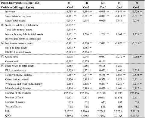
Table 4. Estimation results for Cox models including only accounting ratios.The table shows parameter estimates, standard errors, and model summary statistics for Cox models of the quarterly default intensity of firms in the sample. All variables are lagged one year to allow for one-year prediction. The full list of firm-specific variables are included in model (1). Models (2) through (4) show the stepwise elimination, keeping only the most significant measure within the groups of (1) leverage, (2) profitability, (3) liquidity, and (4) collateralization. Model (5) (shaded grey) is the preferred specification when only firm-specific variables are used as covariates. Significance of parameters is indicated at the 10% (*), 5% (**), and 1% (***) levels. Parameter significance is based on standard errors clustered at the firm-level.

Probability of default and the macroeconomy Thais Lærkholm Jensen

Page | 49

for a correlation matrix of internal variables) the approach has been to perform a stepwise elimination of variables in a given category, removing the least significant variables in each step.18 The outcome is that for the internal variables in the model, interest bearing debt to total assets, net income to total assets, quick ratio and tangible assets (PPE) to total assets remain in the model along with age of banking relationship, log of total assets and a negative equity dummy.

18 _{The stepwise elimination is sensitive to the order of category selection. Performing an alternative specification,}

eliminating variables in the order of (1) profitability, (2) leverage, (3) liquidity and (4) collateralization produce similar results with the only exception of interest payments to total assets showing up in the final model as opposed to interest bearing debt to total asset as in chose specification.

Table 9: Hazard model using only firm specific variables

Dependent variable: Default (0/1)

Variables (all lagged 1 year) Coef Coef Coef Coef Coef

Intercept -6,788*** -6,494*** -6,668*** -6,684 *** -6,729 *** Years active in the bank -0,011*** -0,011*** -0,011*** -0,011 *** -0,011 ***

Log of total assets 0,043 * 0,014 0,020 0,019 0,016

(1) Short term debt to total assets -0,572** Total debt to total assets 0,644 **

Interest bearing debt to total assets 0,661 *** 1,226 *** 1,262 *** 1,261 *** 1,255 *** Interest payments to total assets 7,843 ***

(2) Net income to total assets -0,961** -1,790*** -2,012*** -2,025 *** -2,015 ***

EBIT to total assets 1,403 * 1,963 **

EBITDA to total assets -2,615*** -2,514***

(3) Quick Ratio -0,078 -0,045 -0,057 -0,212 ** -0,202 **

Current ratio -0,192 -0,179 -0,161

(4) Fixed assets to total assets -0,455 -0,288 -0,308 -0,280

PPE to total assets 0,529 ** 0,571 ** 0,473 ** 0,466 ** 0,255 Negative equity, dummy 0,467 ** 0,547 *** 0,555 *** 0,563 *** 0,570 *** Construction, dummy 0,926 *** 0,885 *** 0,928 *** 0,921 *** 0,951 *** Wholesale and retail trade, dummy 0,214 0,216 * 0,267 ** 0,250 * 0,275 ** Manufacturing, dummy 0,404 *** 0,399 *** 0,420 *** 0,406 *** 0,417 *** Number of observations 192.196 192.196 192.196 192.196 192.196

Number of firms 10.671 10.671 10.671 10.671 10.671

Number of events 633 633 633 633 633

Sector effects YES YES YES YES YES

QIC 7.677,2 7.716,4 7.724,8 7.722,8 7.721,9

QICu 7.669,2 7.710,5 7.719,2 7.717,8 7.717,5

Notes: This table presents multiplicative hazard regression models for predicting binary default occurrences by firm specific variables. All variables have been lagged one year to allow for prediction one year out into the future. Data definitions and sources of the time series are given in Appendix 1. The full list of internal variables are included in model (1). Model (2) through (4) is shows the stepwise elimination, keeping only the most significant measure within the groups of (1) leverage, (2)

profitability, (3) liquidity and (4) collateralization. Model (5) (shaded grey) is the preferred baseline specification for firm specific variables. Significance level are represented by *= 10%, ** = 5% and ***= 1%. The significance levels are computed based on clustered standard errors using the PROC GENMOD GEE procedure in SAS.

(5) (4)

(3) (2)

(1)

each step. The outcome is that interest bearing debt to total assets, net income to total assets, quick

ratio, and tangible assets (PPE) to total assets remain in the model, along with age of banking

relationship, log of total assets, and a negative equity dummy.

Interpreting the preferred model (Model 5 in Table 4) the effect of age is negative, implying

that the longer a firm has had a relationship with the bank, the less likely it is that the firm will

default. The effect of size, as measured by book assets, appears insignificant in the specification.

Probability of default and the macroeconomy Thais Lærkholm Jensen

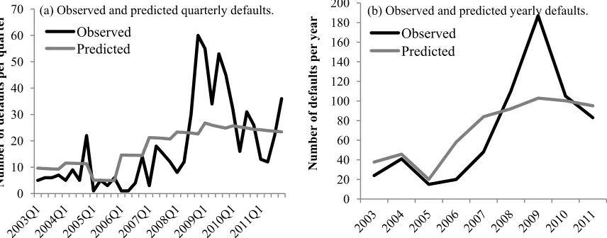
Page | 51 appropriate to aggregate the predicted and observed number defaults in a given year – this is what is shown in panel (b). The conclusion is the same: The model based solely on firm specific variables is not capable of capturing the observed variation in defaults.19

As discussed in the section of estimation methodology, the difference between the discrete Cox regression and a chosen hazard model is expected to be minor. However for completeness, both model (1) and (5) are, as specified, reported in Appendix 7 both using Cox regression and the logistic regression build into SAS. The differences between the models are virtually non-existing.

Figure 10: Observed and predicted default based on firm specific model

Notes: Panel (a) plots the number of defaults predicted defaults by the firm specific model against the observed number of defaults. Panel (b) is equivalent except that aggregation is done on a yearly basis.

5.2

The role of Macroeconomic variables in explaining defaults

Having concluded that firm specific variables are unable to explain the cyclical nature of corporate defaults this section attempts to incorporate macroeconomic effects. In order to assess if macroeconomic variables add explanatory power in explaining default, the preferred model of the firm-specific variables is included in the specifications below.

Cf. Figure 4 in section 2, the expected effect of adding the macroeconomic variables may be thought to influence the default probability directly but also indirectly through firm characteristics. Focusing on the indirect effect through firm-specific variables, the inclusion of macroeconomic variables is thought to be able to influence e.g. firm’s earnings ability, in line with the model of

19 _{This conclusion may also be inferred by studying the explanatory variables medians and means through the}

observations period where only modest variations over time occur. (See Appendix 12). 0

10 20 30 40 50 60 70

N

um

be

r

of

d

ef

au

lt

s

pe

r

qu

ar

te

r (a) Observed and predicted quarterly defaults.

Observed Predicted

0 20 40 60 80 100 120 140 160 180 200

Number

of

defaults

per

ye

ar (b) Observed and predicted yearly defaults.

Observed Predicted

Figure 3. Default prediction based on the preferred Cox model only including accounting ratios. Panel (a) shows the observed number of quarterly defaults in the sample along with the predicted number of defaults based on the preferred Cox model only including accounting ratios (Model (5) in Table4). Panel (b) is similar, except that the aggregation is done on a yearly basis.

This might potentially be explained by the sample pertaining to only the largest corporate clients,

where size is less relevant as an explanation of default. The leverage ratio of interest bearing debt

to total assets is, as expected, positively related to default probability. Likewise, past profitability

is negatively related to default probability. The quick ratio enters with a significant negative sign

confirming the hypothesis that the more liquidity a firm has, the higher its ability to service

unex-pected cash shortfalls which would otherwise have resulted in a default. Tangible assets, measured

as Plant Property and Equipments (PPE) to total assets, does not appear to have a significant effect,

confirming the findings of Bonfim(2009) that tangible assets remain insignificant in explaining

corporate defaults. The negative (book) equity dummy enters with a positive sign in all

specifica-tions, confirming that negative (book) equity is in fact a sign of a firm in trouble and at increased

risk of default. The sign of the sectoral dummies are all positive and significant, confirming that

these sectors have above average default rates.

Using the results of Table 4, we calculate a predicted quarterly default intensity for each firm

in the sample, and then aggregate these to get a predicted aggregate intensity for each quarter.

Figure3shows the observed number of quarterly defaults in the sample along with the predicted

number of defaults based on the preferred Cox model only including accounting ratios. As evident

in panel (a), the model based on accounting ratios alone is unable to explain the cyclical nature of the observed defaults. However, acknowledging that the firm-specific data can only change yearly

through annual financial statements, it may be more appropriate to aggregate the predicted and

observed number of defaults on a yearly basis. This is shown in panel (b), and the conclusion is

the same: The model based solely on firm-specific variables is not capable of capturing the cyclical

Table 5. Estimation results for Cox models with both accounting- and macroeconomic variables.The table shows parameter estimates, standard errors, and model summary statistics for Cox models of the quarterly default intensity of firms in the sample. All variables are lagged one year to allow for one-year prediction. The full list of firm-specific and macroeconomic variables are included in model (6), and model (7) is the preferred specification after stepwise elimination of variables. Model (8) is the preferred specification in Model (7) excluding the firm-specific variables. Significance of parameters is indicated at the 10% (*), 5% (**), and 1% (***) levels. Parameter significance is based on standard errors clustered at the firm-level.

Probability of default and the macroeconomy Thais Lærkholm Jensen

Page | 54

index tend to be negatively linked to defaults illustrating the importance of demand side effects. Capacity utilization is also negatively associated with default occurrences meriting the interpretation that higher level of idle capacity could result in price competition that would ultimately lead a number of firms to default.

Table 10: Including macroeconomic variables into the firm specific hazard model

Dependent variable: Default (0/1) (6) (7) (8)

Variables (all lagged 1 year) Coef Coef Coef

Intercept -13,341 *** -8,051 *** -7,206 ***

Years active in the bank -0,011 *** -0,011 ***

Log of total assets 0,007 0,007

Interest bearing debt to total assets 1,232 *** 1,231 ***

Net income to total assets -1,877 *** -1,877 ***

Quick Ratio -0,200 ** -0,200 **

PPE to total assets 0,282 * 0,281 *

Dummy for negative equity 0,592 *** 0,591 ***

Aggregate quarterly number of Danish bankruptcies 0,005

Danish Real GDP growth -0,027

Export / GDP 9,633 *

Inflation, pct point -0,124

OMX stock market return -0,052 *** -0,045 *** -0,038 ***

OMX stock market volatility -0,119 *** -0,101 *** -0,099 ***

Difference CIBOR - policy rate, pct. Point 1,837 *** 2,006 *** 2,117 ***

Yield curve slope 10y - 3m, pct. Point 0,986 *** 0,588 *** 0,634 ***

Growth in house prices -0,114 *** -0,104 *** -0,115 ***

Change in consumer confidence Indicator -0,110 *** -0,099 *** -0,110 ***

Change in cyclical indicator, construction 0,002

Change in capacity utilization in the industrial sector -0,338 *** -0,300 *** -0,292 ***

Loan growth to non-financial institutions 0,023 **

Stoxx50 stock market return 0,031 *** 0,034 *** 0,029 ***

EU27 Real GDP growth 0,250 *** 0,227 *** 0,213 ***

Number of observations _{192.196 192.196 192.196}

Number of firms _{10.671 10.671 10.671}

Number of events _{633 633 633}

Sector effects _{YES YES YES}

QIC 7.513 7.513,6 8.265,0

QICu _{7.518 7.508,6 8.264,7}

Notes: This table presents multiplicative hazard regression models for predicting binary default occurrences using both firm specific and macroeconomic variables. All variables have been lagged one year to allow for prediction one year out into the future. Data definitions and sources of the time series are given in Appendix X. Model 5 presents the full model with all macroeconomic variables included, where model 29 only presents the significant variables after stepwise elimination of insignificant variables in model 5. Model 31 includes only macroeconomic variables. Significance level are represented by * = 10%, ** = 5% and *** = 1%. The significance levels are computed based on clustered standard errors using the PROC GENMOD GEE procedure in SAS.

6.2

Including macroeconomic variables

Given that firm-specific variables are unable to explain the cyclical nature of defaults in our sample,

this section incorporates macroeconomic effects in our Cox model. In order to assess if

macroeco-nomic variables add explanatory power beyond what is implied by the firm-specific variables, the

preferred model of the firm-specific variables is used as the basis of the covariate specification.

Table 5 presents estimation results for Cox models incorporating macroeconomic variables.

The selection procedure has been to perform a stepwise elimination of insignificant variables until

only significant macroeconomic variables remain in the model. Model (7) is the preferred model including both firm-specific and microeconomic variables, while Model (8) is this preferred model

excluding the firm-specific variables.

The effects of the firm-specific variables remain robust to the inclusion of the macroeconomic

variables. In the preferred model (Model (7) of Table5), the significant macroeconomic variables

are as follows: The return of the OMX stock market index, the volatility of OMX index, the diff

er-ence between CIBOR and the policy rate, slope of the yield curve, change in consumer confider-ence,

change in the capacity utilization, the return of the Stoxx 50 index, and, finally, the European GDP

growth rate. On the other hand, the aggregate number of defaults, the Danish real GDP growth,

exports as a fraction of GDP, inflation, changes in the cyclical indicator for construction, as well as the loan growth to non-financials are all insignificant.

When interpreting the coefficients of the macroeconomic variables in multivariate intensity

re-gression models, one should bear in mind that it would be unrealistic to obtain a completeceteris

paribuseffect of one macroeconomic variable, as this variable cannot be viewed in isolation from

other macroeconomic variables. While not done here, an appropriate interpretation would involve

testing the model from the perspective of internally consistent scenarios of macroeconomic

vari-ables. For instance, a further analysis shows that the volatility of the stock market, the slope of the

yield curve, the return of the Stoxx 50 index, and the European GDP growth rate appear with an

opposite sign in the preferred model compared to a model where they enter separately.

Nonetheless, a positive return of the OMX stock market would, controlling for other

macroe-conomic effects, imply a lower number of default occurrences one year after. An increased spread

between CIBOR and the policy rate would be associated with an increased number of default

oc-currences, thereby supporting the notion that the higher funding costs of the banks would generally

be passed through to clients. Both growth in house prices and changes in the consumer confidence

index tend to be negatively linked to defaults, illustrating the importance of demand side effects.

Capacity utilization is also negatively associated with default occurrences, meriting the

interpreta-tion that higher level of idle capacity could result in price competiinterpreta-tion that would ultimately lead a

Probability of default and the m acroeconom y Thais Lærkholm

Jensen _{Page |}

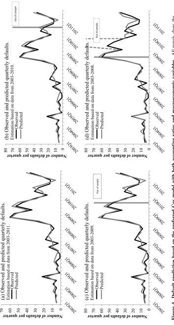
56 Figure 11: Observed and predicted qu arterly defaults based on p re fe rr ed h az ar d m od el f or v ar yi n g u n d er ly in g s am p le s N ot es : T he f ig ur er s (a ), ( b) , ( c) a nd ( d) p lo ts o bs er ve d an d pr ed ic te d qu ar te rl y de fa ul t b as ed o n th e sa m e pr ef er re d ha za rd m od el bu t differen t und erlying samples. ( T he m od el s ar e re por te d in Appendix 14) . The shorter per iod s used for es ti m at io n yi el ds th e pot en tia l f or o ut o f sa m pl e es ti m at io n, w hi ch is th e es ti m at io n don e to the right of th e solid ver tic al li ne. 0 10 20 30 40 50 60 70

80 _{quarter defaults per Number of}

(c ) O bs er ve d an d p re di ct ed q ua rt er ly d ef au lt s. Est im at ion based on dat a from 2003-20 09 . Observed Pred icted 0 10 20 30 40 50 60 70

80 _{quarter defaults per Number of}

(d ) O bs er ve d a nd p re di ct ed q ua rt er ly d ef au lt s. Est im at ion based on dat a from 2003-20 08 . Observed Pred icted Ou t of samp le O ut o f s am pl e O ut o f s am pl e 0 10 20 30 40 50 60

70 _{quarter defaults per Number of}

(a ) O bs er ve d an d p re di ct ed q ua rt er ly d ef au lt s. Est im at ion based on dat a from 2003-20 11 . Observed Pred icted 0 10 20 30 40 50 60 70

80 _{quarter defaults per Number of}

Figure 4 illustrates the relationship between the observed and predicted number of defaults taking into account both the firm-specific variables and the macroeconomic variables in Model (7)

of Table5. Adding macroeconomic variables as explanatory factors improves the model’s ability

to predict the cyclical variation in quarterly default occurrences. To rule out that the good fit of the preferred model is merely a result of over-fitting, the out of sample prediction obtained from

estimating the same model on only part of the data supports the chosen model. Panel (b) and (c) of

the figure estimates the model on the sample excluding observations from 2010 and both 2010 and

2011 respectively. The obtained coefficients from the models estimated on the reduced samples

are then used to estimate the aggregate intensities for all 36 quarters, thereby generating out of

sample predictions. Hence, Panel (b) of the figure shows one and Panel (c) shows two years of

out of sample prediction. The out of sample prediction based on the reduced sample estimation

adequately captures both the level and cyclical variation in default rates.

Panel (d) of Figure 4 shows prediction based on excluding the years 2009, 2010 and 2011

from the estimation. For the out of sample prediction in Panel (d), large deviations occur in 2009

(which pertains to 2008 covariates observations because of the one year lag). However, it should

be emphasized that the latter model has been fitted to a period of economic expansion, and

there-fore it is of little surprise that the model cannot be used to predict future defaults in a period of

economic contraction. This finding also highlights the importance of estimating default predicting

occurrences on a full business cycle.

6.3

Ranking firms with respect to default likelihood

The out-of-sample estimation results presented in Figure4 showed that the preferred Cox model

including both firm-specific and macroeconomic variables adequately captures the level and

cycli-cality of defaults. A common way of illustrating the predictive power of different models based

on the same data is to plot the Receiver Operating Curve (ROC), as shown in Figure5. The curve

illustrates the percentage of defaults that are correctly classified as defaults on the vertical axis

against the percentage of non-defaults that are mistakenly classified as defaults on the horizontal

axis for all possible cutoffpoints. The area under the curve (AUC) is then used as measure of the

model goodness of fit where a value of 1.0 implies a model with perfect discriminatory ability and

a value of 0.5 is a completely random model.

In terms of discriminatory power, the addition of macroeconomic variables does not improve

the model’s ability to effectively determine which firms eventually default beyond what is implied

by the accounting ratios. From the ROC curves, we see that the model with both macroeconomic