A spectral dynamic stiffness method for free vibration analysis of plane elastodynamic problems

City, University of London Institutional Repository

Citation

:

This is the accepted version of the paper.

This version of the publication may differ from the final published

version.

Permanent repository link:

Link to published version

:

Copyright and reuse:

City Research Online aims to make research

outputs of City, University of London available to a wider audience.

Copyright and Moral Rights remain with the author(s) and/or copyright

holders. URLs from City Research Online may be freely distributed and

linked to.

City Research Online: http://openaccess.city.ac.uk/ [email protected]

A spectral dynamic stiffness method for free vibration

analysis of plane elastodynamic problems

X. Liu∗, J.R. Banerjee

School of Mathematics, Computer Sciences and Engineering, City, University of London, London EC1V 0HB, UK

Abstract

A highly efficient and accurate analytical spectral dynamic stiffness (SDS) method for modal analysis of plane elastodynamic problems based on both plane stress and plane strain assumptions is presented in this paper. First, the general solu-tion satisfying the governing differential equasolu-tion exactly is derived by applying two types of one-dimensional modified Fourier series. Then the SDS matrix for an element is formulated symbolically using the exact general solution. The SDS ma-trices are assembled directly in a similar way to that of the finite element method, demonstrating the method’s capability to model complex structures. Any arbi-trary boundary conditions are represented accurately in the form of the modified Fourier series. The Wittrick-Williams algorithm is then used as the solution tech-nique where the mode count problem (J0) of a fully-clamped element is resolved.

The proposed method gives highly accurate solutions with remarkable computa-tional efficiency, covering low, medium and high frequency ranges. The method is applied to both plane stress and plane strain problems with simple as well as complex geometries. All results from the theory in this paper are accurate up to the last figures quoted to serve as benchmarks.

Keywords: Spectral dynamic stiffness method (SDSM), plane stress vibration, plane strain vibration, modal analysis, modified Fourier series, Wittrick-Williams algorithm.

1. Introduction

A wide range of three-dimensional elastodynamic problems are generally treated by two-dimensional (plane) theories, which include plane stress and plane strain theories. The plane stress theory assumes that the stress perpendicular to the plane

∗_{Corresponding author}

under consideration is always zero. This is often the case for plates whose upper and bottom surfaces are free. The vibration of such a plate in its own plane is gen-erally called inplane vibration. Despite the fact that the transverse vibration [1] is usually given more importance for plate-like structures which are more easily excited by transverse external forces rather than inplane forces, there are many instances when inplane vibration can have pronounce effects. As a consequence, there has been an increasing interest in the inplane vibration of plates and plate assemblies. For instance, inplane vibrations are very important for built-up struc-tures [2] where two or more plates are connected at a certain angle such that the transverse and inplane vibrations are directly coupled. The inplane vibrations be-come even more important in the mid to high frequency ranges for noise control and energy transmission analyses of structures [3, 4]. Examples include the walls of aerospace structures, the hulls of ships and cutting tools. The plane strain theory on the other hand, is widely used to investigate the free vibration of engineering structures like earth dams [5], shear wall structures [6] and thin or thick hollow cylinders [7–10]. For example, the earth dams and shear wall structures are de-signed to counter the effect of lateral dynamic loads caused by earthquake or wind. The plane strain theory is also widely used in plane wave propagation problems [11], which have applications in non-destructive testing [12, 13] and phononic crystal analysis [14]. Some other investigators have used the plane strain theory to study the mechanism of edge effects on the natural vibration and wave propaga-tion properties of thick multi-layered plates [15, 16]. As the natural mode shapes can be regarded as the standing waves of a structure with the prescribed bound-ary conditions, the plane strain free vibration can provide important information for wave propagation problems with respect to different boundary conditions or discontinuities.

Without doubt, the above problems can be solved by the finite element method (FEM) with many well-developed commercial packages which can handle com-plex geometries. However, the FEM may become inadequate and unreliable when modelling structures within medium to high frequency ranges. In order to capture the relatively short wavelengths of structural deformations in these frequencies, an FEM model may require prohibitively large number of degrees of freedom (DOF) and even then the results can be still unreliable. Furthermore, for optimisation and parametric studies, the FEM becomes less attractive because of the considerable computational cost and/or the requirement of remeshing the structures. Therefore, analytical methods that are both efficient and accurate should be developed, which will facilitate efficient parametric and optimisation studies by varying significant parameters.

equation [35–37] which governs the transverse vibration of thin plates. The formulated SDS matrices can be assembled directly to allow the modelling of complex geometries just like the FEM, but importantly the adopted shape func-tion in the SDS method (SDSM) is exact instead of approximate as in the FEM. Therefore highly accurate solutions can be obtained from the SDSM by using as few elements as possible. Besides, the SDS formulation represents infinite de-grees of freedom (DOF) accurately and efficiently by using only a very few DOF along the structure boundaries. As a results, the proposed method can provide highly accurate natural frequencies and modal shapes with remarkable computa-tional efficiency, which is much superior to both the convencomputa-tional FEM and BEM, not only within low frequency range, but also within medium to high frequency ranges. Furthermore, the SDSM has the certainty that no natural frequency of the structure will be missed and no spurious modes will be captured. The above superiorities of SDSM plus its analytical essence provide a huge advantage for parametric studies and structural optimisation.

acous-tic performance as well as energy flow properties.

This paper is organised as follows. After this introduction section, the govern-ing differential equation (GDE) and general boundary conditions (BC) are derived by using Hamilton’s principle through a coordinate-free tensor form in Section 2.1. Section 2.2 presents the attainment of exact general solution using two types of modified Fourier series. Then the spectral dynamic stiffness (SDS) matrix for an individual element is formulated through symbolic manipulation; the element SDS matrices can be assembled to form a global SDS matrix to model complex geometries subject to any arbitrary boundary conditions, see Section 2.4. In Sec-tion 2.5, the Wittrick-William algorithm is applied and the so-called J0 count

problem is resolved. Convergence, accuracy and computational efficiency studies are presented in Section 3.1. The theory of this paper is applied to both plane stress (Section 3.2) and plane strain (Section 3.3) problems for benchmark cases as well as engineering applications. Finally, the principal conclusions of this work are reported in Section 4.

2. Theory

2.1. Governing differential equation and general boundary conditions

The governing differential equation (GDE) and the corresponding natural bound-ary conditions (BCs) for plane elastodynamic problems are derived using Hamil-ton’s principle. The application of the HamilHamil-ton’s principle will not only lead to the GDE but also relate the generalised forces and displacements BCs which facilitate the spectral dynamic stiffness (SDS) formulation in the next step. The GDE and BCs are derived in a coordinate-free tensorial form which is applicable to both plane stress and plane strain vibration problems.

Assuming that a three-dimensional (3D) elastic body undergoing vibration de-scribed by the contravariant basis B = {g₁,g₂,g₃} withg₃ ·g₁ = g₃ ·g₂ = 0, the geometry, material properties, deformation and boundary conditions of the 3D body may then be considered not to vary in theg₃direction. Therefore, the defor-mation of the 3D body can be represented by the defordefor-mation of the cross section occupying Ω bounded by∂Ω. Hamilton’s principle for the cross section Ωcan then be written in the usual notation as

δ ∫ t2

t1

(K − W+We)dt= 0, (1)

where Kand W are respectively the kinetic and elastic energies of the body on the cross sectionΩ, andWeis the work done by external loadsqon the boundary

∂Ω(assuming no body force is applied) so that

K= 1 2

∫

Ω

ρu˙ ·u˙dA , W = 1

2

∫

Ω

σ :edA , We=

∫

∂Ω

where ρ is the density of the elastic body; ()˙ denotes the derivative of () with respect to time; e andσ are linear strain and Cauchy stress tensors respectively with

e= 1

2(u⊗∇+∇⊗u) := (∇⊗u)

s

(3)

and

σ =λtr(e)I+ 2µe=λ(∇·u)I+ 2µ(∇⊗u)s (4)

and whereλandµare theeffectiveLam´e constants of the cross section made of a certain isotropic material. Here, λ takes different expressions for plane stress (λe) and plane strain (λa) deformation in terms of engineering elastic constants

E and ν; whereas µ (which is essentially the shear modulus G) takes a unique expression, namely

λ=

    

λe= Eν

1−ν2 plane stress

λa= Eν

(1 +ν)(1−2ν) plane strain

, µ=G= E

2(1 +ν). (5)

It should be mentioned in passing thatλe_orλa_{can be obtained by lettingσ}33 _{= 0}

ore33 = 0, respectively when reducing the Hooke’s law from a 3D problem into a 2D (plane) problem. A close inspection on the Eq. (5) reveals that λa > λe

forν ∈ [0,0.5). It is therefore expected that the natural frequencies for the plane strain deformation will be always larger than those under plane stress deformation when all other factors are identical. Also, it is easily seem that λais the same as that of 3D solid whereasλe_{is somehow different.}

After routine manipulations, Eq. (1) leads to

δ t2

∫

t1

[∫

Ω

(∇·σ−ρu¨)·δudA+

∫

∂Ω

(q−σ·n)·δuds

]

dt = 0. (6)

In view of Eq. (4) and due to the complete arbitrariness of δu, the first terms in the square brackets on the left hand side of Eq. (6) leads to the GDE in the form

∇·σ−ρu¨ = (λ+µ)∇(∇·u) +µ∇2u−ρu¨ =0, (7)

which is the so-called Navier’s equation. Now introducing the local coordinates {n,s} attached to the boundary∂Ωwherenand sare normal and tangent unit vectors forming an orthonormal basis, the second term in the square brackets on the left hand side of Eq. (6) becomes

∫

∂Ω

(q−σ·n)·δuds=

∫

∂Ω

x y z

T1

L1

S1

N1

T2

L2

S2

N2

T3

L3

S3

N3

T4

L4

S4

N4

B1

B2

B3

B4

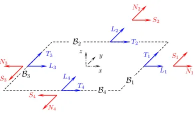
Figure 1: Coordinate system and notations for a rectangular element.

By substituting Eq. (4) into Eq. (8), the natural BCs can now be written in the form

δun: qn =σ·n·n=λ∇·u+ 2µ∇nun = (λ+ 2µ)∇nun+λ∇sus, (9a)

δus: qs=σ·n·s=µ(∇nus+∇sun), (9b)

whereqn =q·nandqs =q·s.

We will first aim to obtain the spectral dynamic stiffness (SDS) matrix of a rectangular element for the plane elastodynamic problems, see Fig. 1, following which, complex geometries will be modelled as an assembly of SDS elements. If Cartesian coordinate system (x, y)is introduced with the origin placed at the centre of the rectangular, so that(x, y) ∈ [−a, a]×[−b, b] = Ωforu = [u, v]T_, the GDE of Eq. (7) becomes

(λ+ 2µ)u,xx+µu,yy+ (λ+µ)v,xy−ρu¨= 0, (10a)

(λ+ 2µ)v,yy+µv,xx+ (λ+µ)u,xy−ρ¨v = 0, (10b)

where the suffix after the comma denotes the corresponding partial derivatives. If harmonic oscillation is assumedu=Uexp(−iωt)whereU = [U, V]T_{, the GDE} in the frequency domain can be derived from Eq. (10) to give

a1U,xx+U,yy+a2V,xy+κU = 0, (11a)

a1V,yy+V,xx+a2U,xy+κV = 0, (11b)

where

a1 =a0 + 2, a2 =a0 + 1, a0 =λ/µ , κ=ρω2/G . (12)

By recalling Eq. (5), a0 (and thereforea1 anda2) will have different expressions

for plane stress and plane stress deformation, namely,

a0 =

    

ae₀ = 2ν

1−ν plane stress

aa₀ = 2ν

1−2ν plane strain

The natural BCs in the frequency domain along the four boundariesBi(i=1,2,3,4) of the rectangular element in Fig. 1 are obtained by applying Eq. (9) to the four boundaries to give

δLi : Ni, δTi : Si, i= 1,2,3,4, (14)

where the direction of Li, Ni, Ti and Si are given in Fig. 1 with the following expressions             L1 T1 L2 T2 L3 T3 L4 T4             =            

U|x=a

V|x=a

V|y=b

U|y=b

U|x=−a

V|x=−a

V|y=−b

U|y=−b

            ,             N1 S1 N2 S2 N3 S3 N4 S4             =G            

(a1U,x+a0V,y)|x=a

(U,y+V,x)|x=a

(a1V,y+a0U,x)|y=b

(U,y+V,x)|y=b −(a1U,x+a0V,y)|x=−a

−(U,y+V,x)|x=−a −(a1V,y+a0U,x)|y=−b

−(U,y+V,x)|y=−b

            . (15)

Here, Li andTi are introduced to denote the normal unand tangent us displace-ments of Eq. (9) respectively along the ith boundaryBi whereas Ni and Si are the longitudinal (qn) and shear (qs) forces along the same boundaries. It is worth emphasising thatLi(Ni)andTi(Si)are defined either byU(σxx)andV(σxy)or by

V(σyy)andU(σxy), depending on the corresponding boundaries. For plane stress vibration which consists of elements of different thicknessesh, the coefficientG

in Eq. (15) will be replaced byGhto incorporate the contribution of thickness in each element.

Next, the exact general solution of Eq. (11) will be derived which provides complete flexibility to describe any arbitrary BCs of Eq. (15).

2.2. Spectral representation of exact general solution and general boundary con-ditions

One of the most challenging problems in the SDSM development is the deriva-tion of the exact general soluderiva-tion of GDE subject to any arbitrary BCs, which is without doubt more challenging than the classical dynamic stiffness method (DSM) development under simply support assumptions. This is because the SDSM is for a real two-dimensional (2D) problem whereas the classical DSM is some-how for a quasi-one-dimensional (1D) problem (either for beam elements or for Levy-type plate elements with a pair of opposite edges simply supported).

(11) rather than only oneW(x, y)encountered earlier in the biharmonic equation. Besides, there is a90◦phase difference betweenU andV in the GDE (11) as well as betweenLi(Ni)andTi(Si)in the BCs, see Eq. (15).

Accordingly, in the current SDSM development for plane elastodynamic prob-lems, two (rather than only one [35–37]) types of modified Fourier basis functions (MFBF) and the corresponding modified Fourier series (MFS) need to be intro-duced. They are given in Section 2.2.1. These two types of MFBF and MFS are adopted not only to obtain the exact general solution of the GDE (Section 2.2.2) but also to transform any arbitrary BCs into the corresponding coefficient vectors, see Section 2.2.3.

2.2.1. Modified Fourier basis functions and the corresponding modified Fourier series

Two types of MFBF and the corresponding MFS are presented in this section, both of which will be used in the SDSM development later in this paper. The first MFBF is the one that was already utilised in the SDSM development for biharmonic equation [35–37], namely

Tl(γlsξ) =

{

cos(γlsξ) l = 0

sin(γlsξ) l = 1

, γls = (s+

l

2)

π

L, (16)

whereξ ∈ [−L, L], s ∈ N = {0,1,2, . . .}. The expressions in Eq. (16) are es-sentially the eigenfunctions of 1D Laplace operator equipped withzero Neumann BCs. This set of MFBF has been proved mathematically [38] to form a com-plete orthogonal set. The corresponding MFS exhibits a much fast convergence rate (asymptotic order two) than the classical Fourier series (asymptotic order one only) when representing analytic, non-periodic functions, see [39]. Indeed, the corresponding MFS is a powerful and elegant tool which partly contributes to the remarkable accuracy and numerical stability of the previous SDSM in [35–37].

However, in the current SDSM formulation for plane elastodynamic problems, apart from the above MFBF given by Eq. (16), another type of MFBF is also required, namely,

T∗

l (γlsξ) =

{

sin(γlsξ) l= 0

cos(γlsξ) l= 1

. (17)

different between U andV and between the BCs. The first few terms of the two types of MFBF are illustrated in Appendix A.

There are different adaptations of modified Fourier series (MFS) correspond-ing to the MFBF described above in Eqs. (16) and (17). In the current SDSM, the following two sets of MFS related to MFBF defined in Eqs. (16) and (17) are proposed. For any 1D arbitrary functionh(ξ), ξ∈[−L, L]subjected to Dirichlet-type BC (with arbitrary Dirichlet BC, i.e., h(±L), but with zero Neumann BC, i.e.,dξh(±L) = 0), one can write

h(ξ) = ∑

s∈N l∈{0,1}

Hls T l(γlsξ) √

ζlsL

, Hls =

∫ L

−L

h(ξ)T√l(γlsξ)

ζlsL

dξ , (18)

where

ζls=

{

2 l = 0ands= 0

1 l = 1ors≥1 . (19)

For any 1D arbitrary function h(ξ), ξ ∈ [−L, L]subjected to Neumann-type BC (with arbitrary Neumann BC, i.e., dξh(±L), but with zero Dirichlet BC, i.e.,

h(±L) = 0), one can write

h(ξ) = ∑

s∈N l∈{0,1}

Hls T∗

l (γlsξ) √

ζlsL

, Hls =

∫ L

−L

h(ξ)T

∗

l (γlsξ) √

ζlsL

dξ . (20)

Similar to [35],√ζlsLis introduced in Eqs. (18) and (20) to eliminate the

depen-dence on the length of the integral range[−L, L]and to retain the symplecticity [40] in the formulated SDSM.

Next, the above two sets of MFBF given by Eqs. (16) and (17) will be applied to derive the exact general solution of the GDE of Eq. (11) and the corresponding two types of MFS in Eqs. (18) and (20) will be used to transform the general BCs given by Eq. (15).

2.2.2. Spectral representation of exact general solution

The exact general solutions for bothU(x, y)and V(x, y)of Eq. (11) can be appropriately expressed by the combination of two series with the aid of the two type of MFBF given by Eqs. (16) and (17) as follows

U(x, y)= ∑ m_∈N k∈{0,1}

T∗

k(αkmx)Ukm(y) + ∑

n_∈N j∈{0,1}

Ujn(x)Tj(βjny), (21a)

V(x, y) = ∑ m_∈N k_∈{0,1_}

Tk(αkmx)Vkm(y) + ∑

n_∈N j_∈{0,1_}

where Tk,Tj and Tk∗,Tj∗ are MFBF defined in Eqs. (16) and (17) respectively with the wavenumbers αkm = (m+k/2)π/aandβjn = (n+j/2)π/b;Ukm(y),

Ujn(x), Vkm(y) and Vjn(x) are 1D functions to be determined exactly from the GDE in the next step. It should be noted here that both U(x, y)andV(x, y)are expressed by the combination of two series: the first series is expanded using the MFBF in x with the corresponding y-components exactly derived from the GDE; the second one is expanded using the MFBF inywith the correspondingx -components exactly derived. The combination of such two series instead of only one is essential to establish a complete solution space for bothU(x, y)andV(x, y)

governed by the GDE of Eq. (11). Another point needs to be emphasised is that the second series ofU(x, y)and the first series ofV(x, y)in Eq. (21) are expressed in terms of MFBF of Eq. (16) whereas the first series ofU(x, y)and the second series ofV(x, y)are expressed in terms of the MFBF of Eq. (17). This is because

U(x, y)andV(x, y)denote the deformations inxandydirections respectively and therefore, have a 90◦phase difference. It will become more transparent in the later formulation that Eq. (21) is indeed the unique expansion which guarantees that the

k andj subscripts will correspond correctly to the symmetric and antisymmetric properties of the related mode shapes.

Now we are in position to derive the unknown functionsUkm(y), Ujn(x), Vkm(y) andVjn(x)of Eq. (21). Substituting Eq. (21) into GDE of Eq. (10) and collecting similar terms of the MFBF yeild the following two ordinary differential equations (ODE) sets

[

d2

y+κ−a1α2_km −µ1dy

µ1dy a1d2y+κ−α2km ] [

Ukm(y)

Vkm(y) ]

=

[

0 0

]

(∀)k∈ {0,1}, m∈Nexceptk=m= 0 (22a)

[

a1d2x+κ−βjn2 µ2dx

−µ2dx d2x+κ−a1βjn2 ] [

Ujn(x)

Vjn(x) ]

=

[

0 0

]

(∀)j∈ {0,1}, n∈Nexceptj=n= 0 (22b)

where di

x = di/dxi, diy = di/dyi and µ1 = (−1)ka2αkm, µ2 = (−1)ja2βjn.

(The two special cases when k = m = 0 and j = n = 0 will be treated at the end of this section.) Notice that Eqs. (22a) and (22b) are simultaneous ODE with constant coefficients, therefore it is appropriate to assume that Ukm(y) =

δkmVkm(y) with Vkm(y) = exp(tkmy) and Vjn(x) = δjnUjn(x) with Ujn(x) =

exp(rjnx). Consequently, the characteristic equations of Eqs. (22a) and (22b) are respectively given by

a1t4km+b2t2km+c2 = 0 (23a)

a1rjn4 +b1rjn2 +c1 = 0 (23b)

where

b2 = (a1+ 1)κ−2a1α2km c2 = (κ−αkm2 )(κ−a1αkm2 ),

It is easily seen that Eq. (23a) has four roots±t1km and±t2kmand Eq. (23b) also has four roots±r1jnand±r2jn, where

t1km

t2km

} =

√ −b2∓

√

b2₂−4a1c2 2a1

, r1jn r2jn

} =

√

−b1∓

√

b2₁−4a1c1 2a1

. (24)

Thus the general solutions forUkm(y), Vkm(y), Ujn(x)andVjn(x)in Eqs. (21) are

{

Ukm(y) =δ1kmC˜1kmch(t1kmy) +δ1kmC˜2kmsh(t1kmy) +δ2kmC˜3kmch(t2kmy) +δ2kmC˜4kmsh(t2kmy)

Vkm(y) = ˜C1kmch(t1kmy) + ˜C2kmsh(t1kmy) + ˜C3kmch(t2kmy) + ˜C4kmsh(t2kmy)

(25a)

{

Ujn(x) = ˜D1jnch(r1jnx) + ˜D2jnsh(r1jnx) + ˜D3jnch(r2jnx) + ˜D4jnsh(r2jnx)

Vjn(x) =δ1jnD˜1jnch(r1jnx) +δ1jnD˜2jnsh(r1jnx) +δ2jnD˜3jnch(r2jnx) +δ2jnD˜4jnsh(r2jnx)

(25b)

whereδikm andδijn (i = 1,2) are obtained by inserting Eqs. (25) into Eqs. (22) to give

δikm=−a1t

2

ikm+κ−α

2

km µ1tikm

, δijn=−a1r

2

ijn+κ−βjn2 µ2rijn

. (26)

Also, the following identities can be obtained based on Eqs. (22)

(a1r2ijn+κ−β

2

jn)(r

2

ijn+κ−a1βjn2 ) +µ

2 2r

2

ijn= 0, (27a) (t2_ikm+κ−a1αkm2 )(a1t2ikm+κ−α

2

km) +µ

2 1t

2

ikm= 0. (27b)

In what follows, the exact general solution obtained above will be partitioned into four symmetric/antisymmetric components. This will be taken advantage of in the subsequent SDSM development leading to analytical expressions by using the two types of MFBF discussed earlier. This procedure will also contribute to the reduction of the computation cost. Thus U(x, y) and V(x, y) given by Eqs (21) and (25) can be decomposed into fourkj components

U(x, y) = ∑

k,j∈{0,1}

Ukj(x, y) = U00+U01+U10+U11, (28a)

V(x, y) = ∑

k,j∈{0,1}

Vkj(x, y)=V00+V01+V10+V11, (28b)

Vk0 are antisymmetric iny (k ∈ {0,1}). In this way,Ukj andVkj can be repre-sented by considering the appropriate symmetric/antisymmetric properties of the MFBF and the hyperbolic functions

Ukj(x, y) = ∑

m∈N  T∗

k(αkmx) ∑

i=1,2

(δikmCikmHj(tikmy))  +∑

n∈N  ∑

i=1,2

(DijnH∗k(rijnx))Tj(βjny)  ,

(29a)

Vkj(x, y) = ∑

m∈N 

_Tk(αkmx) ∑

i=1,2

(

CikmH∗j(tikmy) )_

+∑

n∈N  ∑

i=1,2

(δijnDijnHk(rijnx))Tj∗(βjny)  ,

(29b)

where Cikm and Dijn are unknowns to be determined, and Hk,Hj and H∗k,H∗j stand for hyperbolic functions defined as follows.

Hj(tikmy) =

{

ch(tikmy) j= 0

sh(tikmy) j= 1

, Hk(rijnx) =

{

ch(rijnx) k= 0

sh(rijnx) k= 1

, (30a)

Hj∗(tikmy) =

{

sh(tikmy) j= 0

ch(tikmy) j= 1

, H∗_k(rijnx) =

{

sh(rijnx) k= 0

ch(rijnx) k= 1

. (30b)

Attention should be drawn to the above deduction from Eqs. (22) to (29) for two special cases. Whenk =m = 0andj =n= 0, Eqs. (22a) and (22b) will reduce to second-order equations both of which will lead to two roots±t00and±r00with

t00 =r00 =

√

−κ/a1. (31)

Accordingly, Eq. (25) becomes

Ukm= 0, Vkm = ˜C100ch(t00y) + ˜C200sh(t00y), whenk =m = 0, (32a)

Vjn= 0, Ujn= ˜D100ch(r00x) + ˜D200sh(r00x), whenj =n= 0. (32b)

As a result, when j = n = 0, the zero term (n = 0) of the second series in Eq. (29a) becomesD00H∗0(r00x); whenk =m= 0, the zero term (m= 0) of the first

series in Eq. (29b) becomesC00H∗0(t00y).

2.2.3. Spectral representation of general boundary conditions

Due to the 90◦ phase difference between Li (Ni) and Ti (Si), the two types of MFS of Eqs. (16) and (17) are adopted to transform any arbitrarily prescribed BCsLi, NiandTi, Sirespectively on theith boundaryBi. To this end, one has the corresponding modified Fourier coefficient vectors

where

Ni = [Ni00, Ni01,· · · , Ni0s,· · · , Ni10, Ni11,· · · , Ni1s,· · ·]T , (34a) Si = [Si01,· · · , Si0s,· · ·, Si10, Si11,· · · , Si1s,· · ·]T , (34b) Li = [Li00, Li01,· · · , Li0s,· · · , Li10, Li11,· · ·, Li1s,· · ·]T , (34c) Ti = [Ti01,· · · , Ti0s,· · · , Ti10, Ti11,· · · , Ti1s,· · ·]T . (34d)

Here, the sub-vectors Ni and Li are the modified Fourier coefficient vectors of the BCs onBi of the element by applying the MFS (16) toNi andLi of Eq. (15) respectively, and Si and Ti are the corresponding modified Fourier coefficient vectors by applying the MFS (17) to Si and Ti of Eq. (15) respectively. For example,

Nils =

∫ L

−L

Ni

G

T_√l(γlsξ)

ζlsL

dξ , Tils=

∫ L

−L

Ti T∗

l (γlsξ) √

ζlsL

dξ ,

where l ∈ {0,1}, s ∈ N, ξ denotes either x ory and 2L is the boundary length representing either 2a or 2b in this paper. It should be noted thatSi00 and Ti00

are zero becauseT₀∗(γ00ξ) ≡ 0based on Eq. (17). Therefore, both Si00andTi00

have been deleted from the vectors Si andTi respectively to avoid null rows or columns.

2.3. Development of the spectral dynamic stiffness matrix of an element

The general solution obtained in Section 2.2.2 will serve as the exact shape function to develop the spectral dynamic stiffness (SDS) matrix for an element in this section. The analytical formulation procedure for the plane vibration in this paper is similar to but different from that for the transverse vibration [35]. First, the formulation for the four component SDS matricesKkj is providedin Section 2.3.1. Then, the four component matricesKkjwill be combined in a suitable way to form the complete SDS matrixK for the whole element, see Section 2.3.2.

2.3.1. Development of the SDS component matrixKkj

Essentially, the component SDS matrixKkj relates the generalised displace-ment and force BCs

[Lkj_a , Lkj_b , T_akj, T_bkj]T ,[N_akj, N_bkj, S_akj, S_bkj]T , (35)

This includes two steps. Firstly, all unknown coefficientsC00, C1km, C2km, D00, D1jn

andD2jn in the solution component of Eq. (29) are determined through the

pro-cedure described in Appendix C, which is essentially based on the expressions of

Lkj_a , Lkj_b , S_akj and S_bkj in Eq. (C.1). (Compared to the transverse vibration for-mulation [35], special attention should be paid here in the determination forD00 (whenn = j = 0) andC00(whenk = m = 0). Subsequently, an infinite system

of algebraic equations is derived by substituting the above determined unknowns into the remaining entries Tkj

a , T kj

b , Nakj and N kj

b in Eq. (C.1) and applying the modified Fourier series formula (A.1) to the hyperbolic functions, see Appendix D for details. This infinite system can be rewritten in the following mixed-variable matrix form as: _[

Tkj Nkj

]

=

[

Akj_{T L} Akj_{T S} Akj_{N L} Akj_{N S}

] [

Lkj Skj

]

. (36)

The explicit expressions of the four coefficient matricesAkj_••in Eq. (36) are given in Appendix E, which are concise and easy to be implemented in programming. The sub-vectors of Eq. (36) are defined as

Tkj = [Taj0, Taj1,· · · , Tajn,· · · , Tbk0, Tbk1,· · · , Tbkm,· · ·]T , (37a) Nkj = [Naj0, Naj1,· · · , Najn,· · · , Nbk0, Nbk1,· · · , Nbkm,· · ·]T , (37b) Lkj = [Laj0, Laj1,· · · , Lajn,· · · , Lbk0, Lbk1,· · · , Lbkm,· · ·]T , (37c) Skj = [Saj0, Saj1,· · · , Sajn,· · · , Sbk0, Sbk1,· · · , Sbkm,· · ·]T (37d)

whose entries are the Fourier coefficients in Eq. (C.1). Each entry of the above vectors corresponds to a frequency-wavenumber dependent DOF. It should be noted that when k = m = 0 or j = n = 0, the term Sa00, Sb00 and Ta00, Tb00

in Eqs. (37d) and (37a) are zero and should be removed from the matrices Skj andTkj respectively.Also, themixed formulation of Eq. (36) facilitates resolving the so-calledJ0count problem which will be described later in Section 2.5.

On the basis of Eq. (36), the SDS matrix for eachkjcomponent can be recon-structed in the following form

fkj =Kkjdkj, (38)

in which

fkj =G [

Nkj Skj

]

, dkj =

[

Lkj Tkj

]

, (39)

Kkj =G [

Akj_{N L}−Akj_{N S}Akj_{T S}−1Akj_{T L} Akj_{N S}Akj_{T S}−1 Akj_{T S}−1Akj_{T L} Akj_{T S}−1

]

(Note that the structure of the Kkj above takes different form compared to that in the transverse vibration formulation, i.e., Eq. (29) in [35].) In Eq. (40),Gis the shear rigidity defined in Eq. (5) which results from Eq. (C.1b). As mentioned earlier at the end of Section 2.1,Gwill be replaced byGhin plane stress problems to consider the contribution of different thickness of each element.

2.3.2. Integration of component SDS matrices to the elemental SDS matrix The integration of component SDS matrices to the elemental SDS matrix is similar to that for the transverse vibration [35]. Therefore,f,dof Eq. (33) can be related tofkj,dkjof Eq. (39) in the form

f =T[f00T,f01T,f10T,f11T]T, [d00T,d01T,d10T,d11T]T = 1 2T

T_d.

(41)

However, in Eq. (41), the transfer matrixT is determined by the relationships of Eqs. (B.2) and (B.3) of Appendix B, which takes the different form compared to that in the transverse vibration formulation in [35], namely

T =                            

In O O O O O O O In O O O O O O O

O O O O In O O O O O O OInO O O

O O I†_n O O O O O O O I†_n O O O O O

O O O O O OIn O O O O O O O In O

O Im O O O ImO O O O O O O O O O

O O O O O O O O O Im O O OIm O O

O O OI†_m O O O I†_m O O O O O O O O

O O O O O O O O O O O ImO O O Im

−In O O O O O O O In O O O O O O O

O O O O−InO O O O O O OInO O O

O O I†_n O O O O O O O −I†_n O O O O O

O O O O O OIn O O O O O O O−In O

O −ImO O O ImO O O O O O O O O O

O O O O O O O O O−Im O O OIm O O

O O OI†_m O O O−I†_mO O O O O O O O

O O O O O O O O O O O ImO O O −Im

                            , (42)

whereIn,I†n,ImandI†mare identity matrices of dimensionn, n−1, mandm−1 respectively, and Orepresents null matrices. Finally, puttingEqs. (38), (33) and (41) together yields the SDS matrix for the entire element as

where

K = 1 2T

   

K00 O O O

O K01 O O

O O K10 O

O O O K11

  

TT (44)

is the SDS matrix of the entire element.

2.4. Assembly procedure and the application of any arbitrary boundary condi-tions

One of the major advantages of the current SDSM over other analytical meth-ods lies in the fact that the SDS elements can be assembled to allow the modelling of complex geometries. The assembly procedure from the elemental SDS matri-ces K to form the final SDS matrix Kf is similar to that of the finite element

method (FEM). The only exception is that SDS elements are connected by line nodes whereas the FEM elements are connected by point nodes. The assembly procedure has been described in [36] and will not be repeated here.

The other advantage of the current SDSM over other analytical or numerical methods is that in the SDSM any arbitrary boundary conditions (BCs) can be ap-plied very easily and accurately in the strong form. These BCs can be arbitrarily prescribed ranging from classical, uniform elastic BCs or arbitrary non-uniformly distributed elastic supports, mass attachments as well as elastic coupling con-straints [41]. For plane elastodynamic problems governed by Eq. (11), there are four types of classical BCs. For eachith boundaryBi, one has the following four possible classical BCs

Clamped (C): Li =Ti = 0, (45a) Simply supported 1 (S1): Ti =Ni = 0, (45b)

Simply supported 2 (S2): Li =Si = 0, (45c) Free (F): Ni =Si = 0. (45d)

The final SDS matrixKf of the whole structure can be condensed directly for the DOF fixed with zero displacement. More specifically, the rows and columnsKf which related to Li and Ti will be condensed for ‘C’ boundaries; those related toTi will be condensed for ‘S1’ edges; those related toLi will be condensed for ‘S2’ edges; and of course, no condensation is required for ‘F’ edges.

medium and high frequency ranges. The merits of the SDSM are exploited by the application of the well-known Wittrick-Williams (WW) algorithm [42] which is further enhanced by some novel techniques as described in this section. Suppose that ω denotes the circular (or angular) frequency of a vibrating structure, then according to the WW algorithm, asωis increased from zero toω∗, the number of natural frequencies passed (J) is given by

J =J0+s{Kf}, (46)

where s{Kf} corresponds to the negative inertia of the final SDS matrix Kf

evaluated atω =ω∗; andJ0 is given by

J0 =

∑

m

J0m, (47)

whereJ0mis the number of natural frequencies betweenω = 0andω =ω∗for an

individual component member when its boundaries are fully clamped. For more details, interested readers are referred to [35, 36, 42]. A similar strategy described in [35] is also adopted here to provide an efficient and reliable prediction for the aboveJ0mwhich is based on the closed-form solution of each members subject to

full simple supports. Therefore, J0mof Eq. (47) can be obtained by applying the

WW algorithm in reverse to give

J0m =JSm−s(KSm), (48)

where JSm is the overall mode count of a certain member with all boundaries

subject to simple supports, and s(KSm)is the sign count of its formulated SDS

matrix KSm. In the present method, the strategy based on Eq. (48) has been

successfully implemented using the following steps.

First, the computation of JSm in Eq. (48) is accomplished in an analytical manner by solving a number theory problem. It is well-known that the exact solution for the natural frequency of an all-round simply supported (S2) element

is available [17, 19, 43]. The natural frequencyωmˆˆnfor the case can be expressed analytically in the following nondimensionalised form

2ρ G

(

2aωmˆnˆ π

)2

=a1( ˆm2+η2nˆ2), m,ˆ nˆ ∈ {1,2,3, ...}, (49)

and

2ρ G

( 2aωmˆnˆ

π

)2

0 1 2 3 4 5 6 0

1 2 3 4

ˆ

m2+η2nˆ2=Π1 a₁

ˆ

m

ˆ

n

(a₎JSm₁

0 1 2 3 4 5 6

0 1 2 3 4

ˆ

m2+η2nˆ2= Π1

a₁+2

ˆ

m

ˆ

n

(b₎JSm2

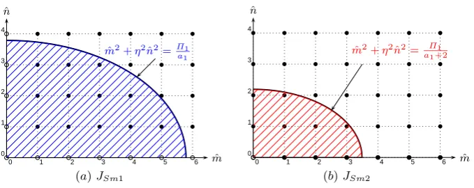
Figure 2: The mode counts JSm1andJSm2 associated with Eqs. (49) and (50) are essentially extended Gauss circle problems illustrated in plots(a)and(b)respectively. Black solid dots are counted whereas empty circles are not counted. In both plots,Π1= 2ρ(2aω∗/π)

2

/G.

whereη =a/bandmˆ andˆnare the number of half-waves in thexandydirection respectively. Thus, JSm, the number of natural frequencies lying below a trial natural frequency ω∗, is essentially the total number of combinations of ( ˆm,nˆ)

such that the left-hand sides of Eqs. (49) and (50) withωmˆˆn=ω∗are not smaller than the right-hand sides. Therefore,

JSm =JSm1+JSm2. (51)

Obviously, JSm1 and JSm2 can be obtained from a numerical search which may

be computationally expensive and the procedure may miss some of the natural frequencies. However, there exists an analytical expression for JSm1 and JSm1

and this problem is essentially an extension of the Gauss circle problem [44] in the field of number theory. In essence, JSm1 is the number of black solid dots

within the blue shaded region covered by the curve mˆ2 +η2nˆ2 = Π1/a1 in Fig.

2(a); whereasJSm2is the number of black solid dots within the red shaded region

covered by the curve mˆ2 _+η2_nˆ2 _{= Π}

1/(a1 + 2) in Fig. 2(b). The analytical

expressions for JSm1 and JSm2 can be deduced by solving the inequalities for

which the left-hand sides of Eqs. (49) and (50) with ωmˆnˆ = ω∗ are greater than

the right-hand sides, hence

JSm1 =

⌊∑Π2⌋

ˆ

m=1

⌊

√ Π1

a1

−mˆ2_/η⌋_{, J}

Sm2 = ⌊∑Π3⌋

ˆ

m=0

⌊

√

Π1

a1+ 2

−mˆ2_{/η+ sign( ˆm)}⌋_,

and

Π1 =

(

2a π

)2

2ρω∗2

G , Π2 =

√ Π1

a1

−η2_{, Π} 2 =

√

Π1

a1+ 2

−η2_.

Next, the computation ofs(KSm)in Eq. (48) is achieved in an elegant way by taking advantage of the mixed-variable formulation explained earlier in Section 2.3.1. Like in [35], when a rectangular element is subjected to all round simple supports as defined in Eq. (45c), the four symmetric/antisymmetric SDS matrices are decoupled. Hence,s(KSm) =

∑

k,j∈{0,1}s(K

kj

Sm).Now recalling Eqs. (38), (39) and (40), the case with fully simple supports of type S2 becomes equivalent

to lettingLkj =Skj =0, such thats(Kkj_Sm) = s(Akj_{T S}−1). In this way, one has

s(KSm) =

∑

k,j∈{0,1}

s(Akj_{T S}−1) = ∑

k,j∈{0,1}

s(Akj_{T S}), (53)

which takes a simpler form than that for the transverse vibration [35] (Eq. 45 therein). The above technique of computingJSmands(KSm)resolves with con-clusive certainty the problem of determiningJ0 in a highly efficient, accurate and

reliable manner. The mode shape computation follows similar procedure as in the SDSM for plate transverse vibration problem [36]. Therefore the details are not given here for conciseness (for more details please refer to [36]).

3. Results and applications

The SDSM described above is implemented in a Matlab program which gives highly accurate solutions for plane elastodynamic problems with remarkable computational efficiency. The convergence, accuracy and numerical efficiency studies are carried out in Section 3.1 below. Then the method is applied to both plane stress problems in Section 3.2 and plane strain problems in Section 3.3.

3.1. Convergence and efficiency investigations for low, medium and high fre-quency modes

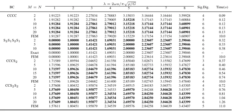
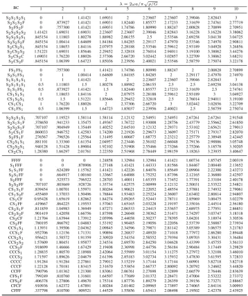
Table 1: Convergence and efficiency studies for the dimensionless natural frequency parameter of a square isotropic plate (ν = 0.3) with four sets of different BCs by using the SDSM. FEM solutions in comparison are obtained by (ANSYS) using a 300×300 meshof Plane 182 elements (each

element has four nodes with two DOFs at each node). The SDSM results for the S2S1S2S1case

are compared with exact solutions. Bold values are those for which the computed eignfrequencies using SDSM converge to the last figures of the presented values.

BC M=N

λ= 2ωa/π√ρ/G

Sig.Dig. Time(s)

1 2 3 4 5 6 7 8

CCCC 2 1.91223 1.91223 2.27834 2.78883 3.15033 3.16444 3.16444 3.59928 4 0.09

5 1.91282 1.91282 2.27861 2.79005 3.15218 3.17143 3.17143 3.60884 5 0.12

10 1.91284 1.91284 2.27861 2.79012 3.15218 3.17144 3.17144 3.60899 6 0.12 15 1.91284 1.91284 2.27861 2.79012 3.15218 3.17144 3.17144 3.60901 6 0.13 20 1.91284 1.91284 2.27861 2.79012 3.15218 3.17144 3.17144 3.60901 6 0.13

FEM 1.91287 1.91287 2.27863 2.79020 3.15229 3.17154 3.17154 3.60907 4 10.0

S2S1S2S1 2 0.00000 1.00000 1.41421 1.69031 2.00000 2.23607 2.23607 2.39046 6 0.32 5 0.00000 1.00000 1.41421 1.69031 2.00000 2.23607 2.23607 2.39046 6 0.33 10 0.00000 1.00000 1.41421 1.69031 2.00000 2.23607 2.23607 2.39046 6 0.38

Exact 0.00000 1.00000 1.41421 1.69031 2.00000 2.23607 2.23607 2.39046 6 –

FEM 0.00000 1.00001 1.41423 1.69031 2.00002 2.23614 2.23614 2.39048 5 10.0

CCCS2 2 1.71589 1.89594 2.04652 2.61358 2.85040 3.02671 3.15582 3.47699 3 0.37

5 1.71596 1.89625 2.04678 2.61394 2.85180 3.02733 3.15932 3.47827 4 0.40

10 1.71597 1.89626 2.04679 2.61396 2.85183 3.02734 3.15932 3.47830 6 0.46 15 1.71597 1.89626 2.04679 2.61396 2.85183 3.02734 3.15932 3.47830 6 0.54 20 1.71597 1.89626 2.04679 2.61396 2.85183 3.02734 3.15932 3.47830 6 0.74

FEM 1.71596 1.89628 2.04682 2.61400 2.85189 3.02745 3.15945 3.47840 4 10.0

CCS2S2 2 1.57608 1.80432 1.95874 2.34519 2.69515 2.84183 3.04571 3.43305 4 0.72

5 1.57609 1.80450 1.95877 2.34533 2.69570 2.84248 3.04628 3.43397 5 0.76 10 1.57609 1.80450 1.95877 2.34534 2.69570 2.84250 3.04628 3.43399 6 0.81 15 1.57609 1.80451 1.95877 2.34534 2.69570 2.84250 3.04628 3.43399 6 1.04 20 1.57609 1.80451 1.95877 2.34534 2.69570 2.84250 3.04628 3.43399 6 1.26

FEM 1.57611 1.80451 1.95879 2.34539 2.69576 2.84258 3.04639 3.43407 5 11.0

efficiency investigations should be carried out. Table 1 shows four sets of results for the free inplane vibration of a square plate (ν = 0.3) with different boundary conditions, namely, CCCC, S2S1S2S1, CCCS2 and CCS2S2. Notice that in this

paper, the letter C and F represent clamped and free edges respectively whereas S1 and S2 denote edges with two types of simple supports: S1 edges having zero

shear displacement and zero longitude forces (see Eq. (45b)) whilst S2 having

both longitude displacement and shear forces being zero, see Eq. (45b). The no-tation comprising four letters successively represent the right, up, left and bottom edges respectively in an anticlockwise sense. The first eight dimensionless natural frequenciesλ= 2ωa/π√ρ/Gare computed by the current SDSM using only one SDS element with different number of terms(M, N)adopted in the series, where

M =N and both vary from 2 to 20. The results are compared with finite element solutions computed byANSYSusing a very fine mesh with300×300 Plane 182 elements. Among the four tabulated cases, closed-form exact solutions are avail-able only for the S2S1S2S1case which all coincide with the current SDSM results.

frequencies is less than half a second. It can be seen from the table that the SDSM takes only5%computation time of the well-developed commercial FEM package

ANSYSwhich meanwhile, provides more accurate results that the FEM. Another important observation can be made is that the SDSM always gives exact results of the S2S1S2S1irrespective of the number of terms adopted in the series. It is found

that this is true for all cases with at least a pair of opposite edges are S2supported.

The reason is due to the fact that the SDSM formulation is based on representing the unknowns of the general solution byLajn, Lbkm, SajnandSbkm, see Eqs. (C.5) and (C.6).

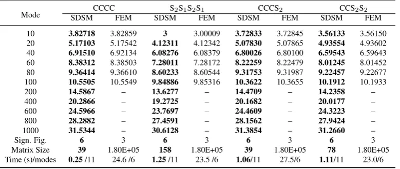
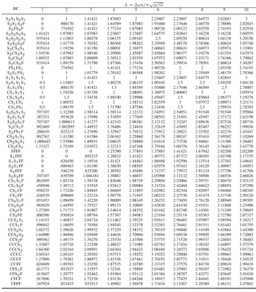
The remarkable accuracy and computational efficiency of the current SDSM is not only evident for low frequency range as shown above but also equally valid for medium to high frequency ranges. This is clear from Table 2 where the SDSM is used to predict the medium (10th-100th) and high (200th-1000th) natural fre-quencies for the same four cases studied earlier in Table 1. When using the SDSM, only one SDS element is used in the modelling with both M and N adopted as 20, and all SDSM results are given with accuracy of six significant figures. The results computed by SDSM are compared with FE solutions computed byANSYS

(using a300×300mesh of Plane 182 elements) with only three significant figures for the 10th-100th modes. Higher natural modes are not computed by the FEM since the solvers provided in the FEM becomes highly inefficient and unreliable for higher modes. The final matrix size and total computational time for both methods are also given in the last two rows of Table 2. To solve the tabulated 11 modes with six significant figures covering medium to high frequency ranges, the SDSM took only 0.25-1.25 s; whereas the well-developed FEM packageANSYS

took 23-28 s but compute only the first six medium modes with three significant figures. It is apparent that SDSM is far more superior to the FEM in free vibration analysis within medium to high frequency ranges. The major advantage of the current SDSM lies in the fact that the SDS formulation satisfies the GDE exactly and uses extremely low number of DOF to represent the system most accurately. For the four case studies shown in Table 2, the final matrix size of the SDSM was only 39-158, which is in a sharp contrast to the FEM which used as many as 1.80E05 DOF. This great advantage establishes the SDSM as an ideal tool for parametric and optimisation studies, not only within low frequency range but also within medium to high frequency ranges.

3.2. Applications to plane stress problems

Table 2: Numerical stability and efficiency studies of the SDSM using the same four cases given in Table 1. The same dimensionless natural frequency parameter as in Table 1 is used, i.e.,λ = 2ωa/π√ρ/G. The SDSM is applied to compute 11 natural frequencies of the four cases covering medium (10th-100th) to higher (200th-1000th) modes. Side by side are the finite element solutions obtained byANSYSusing a300×300mesh of Plane 182 elements, only medium (10th-100th) modes are given for the FE solutions. The final matrix size and the total computational time of both the SDSM and FEM are given in the last two rows.

Mode _SDSMCCCC_{FEM SDSM}S2S1S2S_FEM1 _SDSMCCCS2_{FEM SDSM}CCS2S2_FEM

10 3.82718 3.82859 3 3.00009 3.72833 3.72845 3.56133 3.56150

20 5.17103 5.17542 4.12311 4.12342 5.07830 5.07865 4.93554 4.93602

40 6.91510 6.92134 6.08276 6.08379 6.80026 6.80100 6.59543 6.59643

60 8.38312 8.38503 7.28011 7.28172 8.22259 8.22479 8.01245 8.01452

80 9.36414 9.36610 8.60233 8.60544 9.31753 9.31987 9.22457 9.22677

100 10.5505 10.5549 9.84886 9.85316 10.3622 10.3655 10.1912 10.1933

200 14.5867 – 13.6277 – 14.4709 – 14.2358 –

400 20.2866 – 19.2725 – 20.1682 – 20.0177 –

600 24.5966 – 23.7697 – 24.4609 – 24.3223 –

800 28.2882 – 27.4591 – 28.1562 – 27.9424 –

1000 31.5344 – 30.6128 – 31.3854 – 31.2660 –

Sign. Fig. 6 3 6 3 6 3 6 3

Matrix Size 39 1.80E+05 158 1.80E+05 39 1.80E+05 78 1.80E+05 Time (s)/modes 0.25/11 24.6 /6 1.25/11 23.5 /6 1.06/11 27.5/6 1.11/11 23.0/6

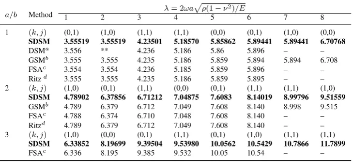
The free inplane vibration analysis of plates has received much less attention compared to the out-of-plane free vibration analysis. There are only a few at-tempts in the literature using different methods which makes the current analysis even more important. As the first example, the current SDSM is applied to the free inplane vibration analysis of a fully clamped plate with different aspect ratios. Ta-ble 3 compares the first eight natural frequencies computed by the SDSM results with those obtained by other methods wherever available. The comparative meth-ods include dynamic stiffness method based on the superposition method (DSM) [31], Gorman’s superposition method (GSM) [18], Fourier series based analytical method (FSA) [32] and the Ritz method [23]. The current SDSM results, which are accurate up to the last figures quoted with six significant figures, are intended to serve as benchmark solutions. It can be found that the results computed by GSM [18] and Ritz method [23] have four significant figures which all coincide with the first four digits of the current SDSM results. The dynamic stiffness method based on the superposition method [31] appears to miss the repeated natural frequency for the square plate as denoted by ‘∗∗’ in Table 3. This might be due to the reason that determinant method rather than the WW algorithm was applied as the solution technique in this method [31]. (Although WW algorithm was mentioned briefly in the context of [31], it is apparent that the WW algorithm was after all not applied in its calculation, let alone how the important issue in the WW algorithm, theJ0

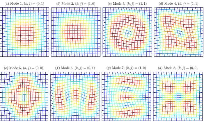
square isotropic plate (a/b= 1) are plotted in Fig. 3 with the(k, j)notation given as follows: (0,0) modes are doubly symmetric about both x and y axes (Figs. 3(e)and(h)) whereas(1,1)modes are double antisymmetric modes (Figs. 3(c)),

(0,1)modes are symmetric in xbut antisymmetric iny(Figs. 3(a)and(f)) and

(1,0)modes are antisymmetric in xbut symmetric in y(Figs. 3(b)and (g)). It should be noted that the(k, j)notation here is different from the ‘S’/‘A’ notation used by Gorman in [18]. As evident from Fig. 3, the(k, j)notation in this paper is more physically meaningful than that by Gorman [18] as the(k, j)in the current SDSM represents the actual symmetric or antisymmetric properties of the defor-mation. Moreover, it can be seen that the 1st and 2nd modes are longitudinally dominant whereas the 3rd mode is shear dominant. Other modes are somehow coupled modes of both longitudinal and shear deformation.

Table 3: The first eight dimensionless inplane natural frequencies of fully clamped isotropic rect-angular plates with three different aspect ratios (a/b). The notationsk(corresponding toxaxis) andj (corresponding toyaxis) of(k, j)denote symmetric (taking ‘0’) or antisymmetric (taking ‘1’) deformation with respect to the corresponding axes.

a/b Method λ= 2ωa

√

ρ(1−ν2_)/E

1 2 3 4 5 6 7 8

1 (k, j) (0,1) (1,0) (1,1) (1,1) (0,0) (0,1) (1,0) (0,0)

SDSM 3.55519 3.55519 4.23501 5.18570 5.85862 5.89441 5.89441 6.70768

DSMa _{3.556 ** 4.236 5.186 5.86 5.896 – –}

GSMb _{3.555 3.555 4.235 5.186 5.859 5.894 5.894 6.708}

FSAc _{3.554 3.554 4.236 5.185 5.859 5.896 – –}

Ritzd _{3.555 3.555 4.235 5.186 5.859 5.895 – –}

2 (k, j) (1,0) (0,1) (1,1) (0,0) (0,1) (1,1) (1,1) (1,0)

SDSM 4.78902 6.37856 6.71212 7.04875 7.6083 8.14019 8.99796 9.51559

GSMb _{4.789 6.379 6.712 7.049 7.608 8.140 8.998 9.515}

FSAc _{4.788 6.374 6.710 7.048 7.608 8.140 – –}

Ritzd _{4.789 6.379 6.712 7.049 7.608 8.140 – –}

3 (k, j) (1,0) (0,0) (0,1) (1,1) (0,1) (1,0) (1,1) (1,1)

SDSM 6.33852 8.19699 9.39504 9.53980 10.0562 10.5429 10.7866 11.7899

FSAc 6.336 8.195 9.385 9.532 10.05 10.54 – –

a_{Dynamic stiffness method based on the Gorman’s superposition method [31]} b_{Gorman’s superposition method [18]}

c_{Fourier series based analytical method [32]} d_{Ritz method [23]}

Ap-(a) Mode 1, (k, j) = (0,1) (b) Mode 2, (k, j) = (1,0) (c) Mode 3, (k, j) = (1,1) (d) Mode 4, (k, j) = (1,1)

(e) Mode 5, (k, j) = (0,0) (f) Mode 6, (k, j) = (0,1) (g) Mode 7, (k, j) = (1,0) (h) Mode 8, (k, j) = (0,0)

Figure 3: The first eight natural mode shapes of a fully clamped plate under free inplane vibration. The(k, j)notation was given in the caption of Table 3. The colour of the mesh, varying from blue to red, indicates the normalised displacement amplitude√U2_+V2_/max(√_U2_+V2_)varying from 0 to 1.

Table 4: The first eight non-zero dimensionless inplane natural frequencies of completely free isotropic rectangular plates (ν = 0.3) with three different aspect ratiosa/b. The(k, j)notation is the same as that given in Table 3.

a/b Methods λ= 2ωa

√

ρ(1−ν2_)/E

4 5 6 7 8 9 10 11

1 (k, j) (1,1) (0,1) (1,0) (0,0) (0,0) (0,0) (0,1) (1,0)

SDSM 2.32060 2.47162 2.47162 2.62845 2.98739 3.45224 3.72312 3.72312

DSMa _{2.320 2.472 ** 2.628 2.988 3.452 3.724 **}

GSMb _{2.320 2.472 2.472 2.628 2.988 3.452 3.724 3.724}

FSAc _{2.321 2.472 2.472 2.629 2.988 3.452 – –}

Ritzd _{2.321 2.472 2.472 2.628 2.987 3.452 – –}

2 (k, j) (0,1) (0,0) (1,1) (1,1) (0,1) (0,0) (1,0) (1,0)

SDSM 1.95365 2.96082 3.26705 4.72633 4.78411 5.20446 5.25689 5.36510

GSMb _{1.956 2.960 3.268 4.726 4.784 5.208 5.258 5.370}

FSAc _{1.954 2.961 3.268 4.725 4.785 5.205 – –}

Ritzd _{1.954 2.961 3.267 4.726 4.784 5.205 – –}

3 (k, j) (0,1) (0,0) (1,1) (0,1) (1,1) (1,0) (0,1) (1,1)

SDSM 1.57065 2.98313 3.22219 4.9479 5.75158 5.82971 7.08253 7.21869

FSAc 1.571 2.983 3.224 4.951 5.754 5.83 – –

a_{Dynamic stiffness method based on Gorman’s superposition method [31]} b_{Gorman’s superposition method [18]}

c_{Fourier series based analytical method [32]} d_{Ritz method [23]}

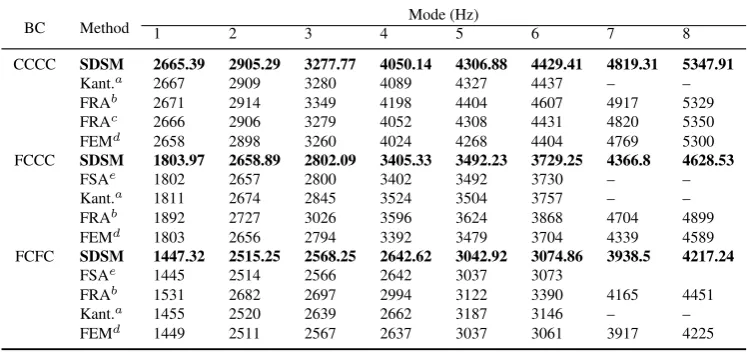
Table 5: The first eight inplane natural frequencies (Hz) of a rectangular plate with three different boundary conditions.

BC Method _{1 2 3 4} Mode (Hz)_{5 6 7 8}

CCCC SDSM 2665.39 2905.29 3277.77 4050.14 4306.88 4429.41 4819.31 5347.91

Kant.a _{2667 2909 3280 4089 4327 4437 – –}

FRAb 2671 2914 3349 4198 4404 4607 4917 5329 FRAc _{2666 2906 3279 4052 4308 4431 4820 5350}

FEMd 2658 2898 3260 4024 4268 4404 4769 5300

FCCC SDSM 1803.97 2658.89 2802.09 3405.33 3492.23 3729.25 4366.8 4628.53

FSAe _{1802 2657 2800 3402 3492 3730 – –}

Kant.a _{1811 2674 2845 3524 3504 3757 – –}

FRAb _{1892 2727 3026 3596 3624 3868 4704 4899}

FEMd 1803 2656 2794 3392 3479 3704 4339 4589

FCFC SDSM 1447.32 2515.25 2568.25 2642.62 3042.92 3074.86 3938.5 4217.24

FSAe _{1445 2514 2566 2642 3037 3073}

FRAb 1531 2682 2697 2994 3122 3390 4165 4451 Kant.a _{1455 2520 2639 2662 3187 3146 – –}

FEMd 1449 2511 2567 2637 3037 3061 3917 4225

a_{Kantorovich method [29]} b_{Forced response analysis 1 [28]} c_{Forced response analysis 2 [27]}