D
EPARTMENT OF
E
CONOMICS
U
NIVERSITY OF
S
TRATHCLYDE
G
LASGOW
THE GAINS FROM ECONOMIC INTEGRATION
B
Y
DAVID COMERFORD AND JOSE V RODRIGUEZ MORA
N
O
17-15
S
TRATHCLYDE
The Gains from Economic Integration
∗
David Comerford
University of Strathclyde
Jos´
e V. Rodr´ıguez Mora
University of Edinburgh
November 21, 2017
Abstract
This paper measures the effect of political integration, such as sharing a national state or economic union, on the degree of trade integration. Consistently with previous work, we find large border effects. However, such estimates may be biased and overestimate the effects of borders because of endogeneity: selection into sharing a political space is correlated with affinities for trade. We propose a method to address this and to estimate a causal effect. We then conduct speculative exercises showing the costs and benefits of the changing levels of integration associated with: the independence of Scotland, Catalonia and the Basque Country from the UK and Spain (but remaining within the European Union); the UK’s exit from the EU; the break-up of the EU itself; and the achievement of frictions between members of the EU similar to those expected between regions of a single country. We find that the border effect between countries is an order of magnitude larger than the border effect associated with the European Union.
Key words: Border effect, trade, independence. JEL Classification: F15, R13
∗We thank Doireann Fitzgerald, Tim Kehoe, Nick Meyers, Pau Pujolas, Robert Zymeck and seminar participants
1
Introduction
The aim of this paper is to measure the effect of political integration, such as sharing a national state
or economic union, on the degree of trade integration, and to quantify its welfare implications. We
definethe economic integrationas the causal effect of sharing political space - this is the additional
welfare gained by entities which come together to form a country or an economic union, due to
increased trade.
We calibrate a structural trade model to interregional and international trade data, and obtain
the implicit trade frictions that would explain the observed data, something often referred to as the
Head Ries Index (HRI)1. We do this while treating countries and sub-national units for which we
have data, as entities with the same status within a common framework. The average border effect
is then the average difference between the interregional and the international frictions, controlling
for physical distance, common language, and size. Likewise the average effect of the European
Union is the average difference between frictions within and across the EU boundary, controlling
for those same characteristics. The existence of very large border effects, even within the European
Union, is well known2 and in this paper we also find large average border effects.
Our main point though is that these average border effects are bound to overestimate the gains
from sharing a state. This is because places which share larger affinities are more likely to both
trade with each other and to select into sharing a political space (a country, or EU membership).
Due to this endogeneity the average effect likely overstates the reductions in trade frictions achieved
by sharing a political space.
For instance, the fact that Scotland and England share a country is related to the fact that
they trade a lot - but we cannot claim that the high volume of trade is all caused by the fact of
1According toHead and Mayer(2013),Eaton, Kortum, Neiman, and Romalis(2011) coin the label “Head-Ries Index” since this “indicator first appears inHead and Ries(2001)”.
state sharing. Scotland and England would trade at a relatively high rate even if they did not
share a country. The affinities that lead to trade between the two also increase the likelihood of
nation state sharing. The causal effect of nation state sharing can be quantified by only changing
the status of state sharing or not - not by also changing these affinities. Looking at the average
difference in trade within and across national borders, even when controlling for physical distance
and common language, does not compare like with like in terms of these affinities. The average
friction between the UK with the rest of the countries of the world, after controlling for physical
distance, size and language, is much larger than the frictions that plausibly would exist between
Scotland and England in the case of independence, even if in that case the frictions were larger
than the ones that we observe today. To impute the difference between the current
Scotland-England frictions with the average frictions that the UK has with other countries as the benefits
of economic integration is likely to overestimate the potential trade benefits of a political union.
Our approach to deal with this endogeneity problem has a certain resemblance to regression
discontinuity analysis. We identify “marginal regions”, defined as regions or countries which seek
to exit the political space under consideration (e.g. Scotland seeking independence from the UK,
or the UK seeking to exit the EU). We also identify“marginal countries”, based on the countries
with the smallest frictions with the country to which the “marginal region” currently belongs (e.g.
Ireland is the natural counterfactual to Scotland with respect to the UK). Essentially “marginal
regions” are regions of a larger country that could conceivably be independent, and “marginal
countries” are independent countries that could easily be regions of the larger country. This
comparison should be clean of the endogeneity problem insofar as the ex-ante probabilities for the
“marginal country” and the “marginal region” to form a political union to the country to which the
“marginal region” belongs, are similar. This comparison gives us our estimate of the causal impact
of sharing political space. Conducting counterfactual exercises based on the difference in frictions
between “marginal region” and “marginal country” allows us to quantify welfare implications.
For example we use the difference between the measured Scotland-rest of the UK friction,
and the measured Ireland-UK friction (because Ireland is observed to have the lowest measured
measured friction with the UK, Ireland is similar in size to Scotland, shares a common language
with Scotland and the rest of the UK, is contiguous with the UK (via Northern Ireland), and
shares much common history (including formerly being part of the UK) - and so we observe that
our methodology produces appropriate and interesting counterfactuals.
Another issue that needs to be considered is the potential for regions to substitute integration
with the rest of their country in place of close links with the rest of the world. For the marginal
regions in our analysis, we show that this is not the case and that the frictions that these regions
have with the rest of the world are in line with those of similarly sized countries. In this sense,
economic integration is a gain: it is not achieved at the expense of higher frictions with the rest
of the world.
We conduct speculative exercises to illustrate the quantitative importance of economic
integra-tion. We consider the independence scenarios for Scotland, Catalonia, and the Basque Country,
as well as looking at “Brexit”: the exit of the UK from the European Union. Furthermore we
look at combinations of these such as Scotland staying in the EU by becoming independent as the
rest of the UK undergoes Brexit. Finally, we consider scenarios which look at the disintegration
of the EU, as well as the possibility that the EU furthers its degree of economic integration across
countries to the same level that there is within its member states.
Welfare impacts can easily be quantified following the contribution ofArkolakis, Costinot, and
Rodr´ıguez-Clare (2012) who show that the total welfare gains from trade, subject to parameters,
are the same in all trade models within the class of ‘gravity models’, and given by a simple formula3.
The productivity or welfare implications of changes in trade frictions can be examined using policy
experiments, and this has been done in many papers in the literature4. In this paper we evaluate
3Though particular microfoundations are suggestive of particular values for the trade elasticity parameter and so do matter, a point made byMelitz and Redding(forthcoming). The microfoundations can be very different, e.g.: a love of variety means that the available product range expands with the size of the market and leads to aggregate increasing returns to scale, as inKrugman(1980); a larger market can lead to better firm selection as efficient firms expand to serve this larger market, putting upward pressure on wages, and lowering profitability of low productivity firms who exit, as in Melitz(2003); and traditional Ricardian trade explanations as inEaton and Kortum(2002). All imply different structural interpretations, and different values, for the trade elasticity. Simonovska and Waugh
(2013) estimate different values for the trade elasticity based on different structural models. Further, the simple formula is different for different sub-classes of gravity models: in this paper we use a gravity model with tradable intermediate goods as discussed in Section IV ofArkolakis, Costinot, and Rodr´ıguez-Clare(2012).
the welfare impacts of changing frictions by the magnitude measured between our marginal regions
and marginal countries as a good estimate of the causal impact of state sharing. We find that,
for all the examples that we look at, the difference for marginal regions in having their measured
interregional frictions and the smallest measured international frictions, accounts for between one
third and one half of the total gains from trade relative to autarky. This is irrespective of the
particular gravity model used (within a subset of the gravity model class), and highly insensitive
to the chosen value for the trade elasticity parameter.
We show that the average econometric estimation exercise (not taking into account the
endo-geneity) over-estimates the causal effect of sharing a country upon economic integration.
Neverthe-less, the value of such economic integration once controlling for this endogeneity is still substantial.
Belonging or not to the EU also has quantitatively significant welfare effects, but these are observed
to be almost an order of magnitude less significant than the impact of sharing a country.
We do not explain the institutional arrangements or mechanisms that lead to economic
integra-tion within countries, we simply identify the size of this integraintegra-tion, and quantify its importance
within a modern general equilibrium model of trade. The differences in the degree of economic
integration may be due to many reasons: biases in government procurement5, home bias in
pref-erences, regulation favouring local firms, political economy biases, migratory patterns, network
formation, etc. In this paper we simply point the facts and leave the investigation of potential
causes to further research6.
* * * * *
We begin our analysis with an illustration showing that something happens within countries
that is different from what happens across countries: the patterns of trade for regions that very
model); and Corcos, Gatto, Mion, and Ottaviano (2012) (examines a number of policy experiments including undoing non-tariff barrier liberalisations associated with EU membership, implementing 5% tariff barriers on trade with the world outside EU, and implementing 5% tariffs on all international trade). Head and Mayer(2013) provide a toolkit for implementing such policy experiments in general equilibrium.
5In a recent paper,Herz and Varela-Irimia(2016) using the universe of public procurement contracts within the EU show that the nationality of the winner of the contract (the supplier) is its most salient characteristic. The border effect in public procurementwithin the EU is enormous, in spite of being explicitly prohibited by the Union treaties to discriminate in favor of domestic suppliers.
6A recent literature on internal frictions is also helpful in moving forward this research agenda, for exampleAtkin and Donaldson(2014),Cosar, Grieco, and Tintelnot(2014), andRamondo, Rodr´ıguez-Clare, and Sabor´ıo-Rodr´ıguez
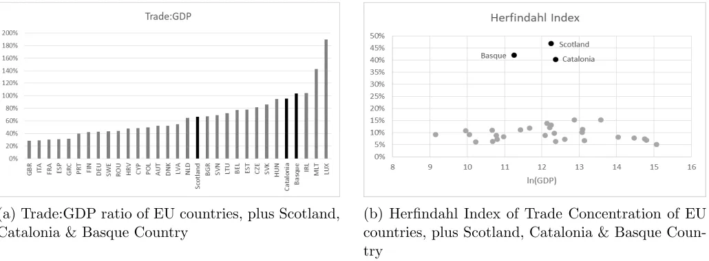
(a) Trade:GDP ratio of EU countries, plus Scotland, Catalonia & Basque Country
[image:7.612.59.574.43.233.2](b) Herfindahl Index of Trade Concentration of EU countries, plus Scotland, Catalonia & Basque Coun-try
Figure 1: Trade and trade concentration in regions and countries
plausibly could be independent countries are very different from those of independent countries.
These regions exhibit a very high degree of trade concentration that marks them out as very
different from otherwise similar countries within the EU. Scotland, Catalonia, and the Basque
Country could be countries, but if they were, we would not expect to see their trade patterns
be as shown in Figure 1. These regions, viewed as if they were countries, appear to be highly
integrated into the global economy with a high share of trade in GDP, however this trade is
extremely concentrated with the rest of the country of which they are currently part. Figure
1a7 shows that the trade share of these regions is typical in a European context, but Figure 1b
highlights how anomalous these regions’ trade concentrations are compared with EU countries. It
shows the Herfindahl index of trade concentration8 against GDP on the x-axis, since we may expect
small countries to trade more, and concentrate this trade with their large neighbours. We would
expect regions to have relatively high index values, as they are relatively small, but not nearly as
high as we observe. The regional Herfindahl Indices are much higher than that of the most trade
concentrated independent EU member9: it’s almost an order of magnitude type comparison. Our
exercise will consist of building reasonable counterfactuals for these regions where they appear as
7The data used in for these graphs, and throughout the paper, is described in Appendix A 8If there areN countries, with the exports from countryito countryjdenotedXi
j (Xii≡0), then the Herfindahl
Index for countryi,Hi=PNj=1[(Xji/
PN
k=1[X
i
k])2]. Hi= 1 indicates complete concentration of trade with a single
trading partner. Hi→0 (equality only possible with infinitely many possible trading partners) indicates complete
diversification of trade across all partners.
normal countries.
The paper is structured as follows. In Section 2 we develop the Head Ries Index framework
for measuring trade frictions, present our cross country and region comparison results (including
some interesting results on the differences in the degree of home bias between trade in goods and
trade in services), and show the (unsurprising) result that a large border effect exists. Section 3
develops our argument on the endogenous selection of economies into regions and countries - the
average border effect is an upwardly biased estimate of the causal effect of the impact of political
integration upon trade frictions. In this section we also describe our method of dealing with this
selection bias. In Section 4 we conduct counterfactual experiments on regional borders in which
we show that, even after allowing for this selection bias, a substantial causal impact remains. The
value of integration across the European Union is considered in Section 5, in which we provide
some quantification for the costs of Brexit. Section 6 concludes.
2
Measuring Trade Frictions
In this section we show that the border effect, understood as the average difference in bilateral
frictions between interregional and international pairs within the EU, is very large. Furthermore,
the EU border effect, understood as the average difference in bilateral frictions between EU pairs
and other country pairs, is smaller but still significant. Differences of the magnitudes that we
obtain have quantitatively significant welfare implications if they are interpreted as the causal
effect of borders.
We perform a simple econometric exercise, regressing for all pairs of countries and regions, the
Head Ries Index measured for each bilateral pair, against the incomes of each party, the physical
distance between them (and this distance squared), a common language dummy, regional border
dummies, and a non-EU border dummy10. The Head Ries Index (HRI) is the well known indicator
10This is equivalent to running a gravity regression of bilateral trade on GDPs and upon dummies for i and j, and explanatory terms for trade frictions: lnXij−lnYi−lnYj = αidi+αjdj+(β1B1+...+βnBn) where dk is a dummy variable for k, and so αk gives its multilateral resistance, and where is the trade elasticity and B1, ..., Bnarenfactors with which we try to explain trade frictions. Sinceδijis a quantity that already incorporates
of trade frictions implied by all gravity models of trade, it is the friction that would produce the
observed bilateral trade within such a gravity model (for a certain trade elasticity). It is a very
natural and theory compatible measure of trade frictions, and has been used many times in the
literature11. It is given by the following expression, where is the trade elasticity, and it is the
same in all models that produce a gravity equation.
δij =
X2 ij XiiXjj
21
(1)
First we outline the data, and then we describe the results of our exercise.
2.1
Data & Methodology
The data used in this paper is fully described in Appendix A. But briefly it is: international data
from the WIOD database covering both goods and services; regional data for the USA, Canada,
Spain, and Scotland, is taken from local statistical agencies; international, Scottish, and US data
is from 2014; Canadian data is from 2013; Spanish (goods only) and Basque (goods and services)
data is from 2006; and Catalan (goods and services) data is from 2005. The following procedure
is followed to construct an internally consistent dataset:
• From the international data we have: Xji, the trade flow from i to j; the Gross Output,Xi,
and theGDPi, for all countriesi∈ {1, ..., N}.
11Chen and Novy (2012) label this approach to trade friction measurement as the “Indirect Approach”. Other papers which have used this approach includeHead and Ries(2001),Eaton, Kortum, Neiman, and Romalis(2011),
• Then define:
β =
P
i(Xi−GDPi) P
iXi
(2)
Xij =
1 2 X
j i +X
i j
(3)
Xii = Xi − X
j6=i
Xij (4)
Yi = (1−β)Xi (5)
• For each region in our data, we construct a data pair comprising of the region and a virtual
“rest of the country”, by applying the share of income, the share of external trade, and the
ratio of internal trade to external trade, implied by the regional dataset, to the output and
international trade from the country dataset12.
Note that when we try to measure trade frictions consistently across countries and regions and
to conduct some basic statistical analysis on these measures, the US states supply the bulk of our
regional data points. The US and Spanish regional trade datasets are for goods trade only. We
therefore use goods only data for Canada despite goods and services data being available, and we
exclude Scotland from the database at this stage. We use the ratio of, say, Texas goods trade with
the rest of the USA to its goods trade with the rest of the world, combined with the Texan share
of US goods trade with the rest of the world, to generate a consistent measure of Texas’s internal
trade, from the USA’s external combined goods and services trade. Given data limitations, this is a
reasonable procedure. But we can infer in which direction it biases our results from the Canadian,
Basque, and Catalan data, and it seems to matter quantitatively - we will come back to this. In
Section 4 we use goods and services data for Scotland, Catalonia, and the Basque Country13.
12For example, Catalan output is given by Spanish output from the cross-country dataset multiplied by the ratio of Catalan GDP to Spanish GDP from the regional dataset. Catalan trade with the rest of the world is given by this Catalan output multiplied by the Catalan external trade to output ratio. Catalan trade with the rest of Spain is given by this Catalan external trade multipled by the internal to external trade ratio. Finally, the figures for the rest of Spain are given by the Spanish figures less the Catalan ones.
To calculate the HRI for the countries and regions in our dataset, we must choose a trade
elasticity, . There is much discussion in the literature (see e.g. Simonovska and Waugh (2013)
and Melitz and Redding (forthcoming)) about the appropriate value for the trade elasticity, but
based loosely onSimonovska and Waugh(2013), for this exercise we choose=−3.514. In Section
4 we will reach a conclusion that is extremely insensitive to this choice.
2.2
Average Border Effect Results
We take logs of the set of calculated HRIs and regress against log of gross output, distance, distance
squared, common language and border dummies.
We have three different types of border dummies. The regional border dummy takes value
1 only if it is a border between regions of the same country. The non EU border dummy takes
value 1 only if it is a border between a non EU country and another country (EU or not). Finally,
we include separate dummies for Canadian and Spanish region to region borders to account for
country fixed effects representing differential levels of internal integration between the US, Canada,
and Spain.
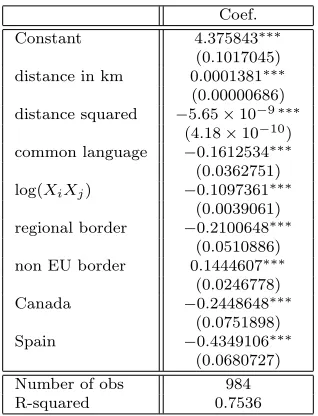
These results are shown in Table 1. They suggest that US internal borders are substantially
less frictional than country to country borders within the EU, that Canadian internal borders are
less frictional than US internal borders, and that Spanish internal borders even less so. Moreover,
the borders between two EU countries are 14% less frictional than borders external to the EU
(where external means that at least one of the parties is not an EU member).
Note that the results in this table are highly dependent on the value of the trade elasticity,
though the significance of each factor is insensitive to this parameter.
Figure 2 shows the measured values of the HRI, adjusted for the impact of physical distance
and common language (i.e “log residual delta” is the log of the regression residual plus the impact
of size and borders, and these are graphed against size), separating out the regions-rest of country
Coef. Constant 4.375843∗∗∗
(0.1017045) distance in km 0.0001381∗∗∗
(0.00000686) distance squared −5.65×10⁻⁹∗∗∗
(4.18×10⁻¹⁰)
common language −0.1612534∗∗∗
(0.0362751) log(XiXj) −0.1097361∗∗∗
(0.0039061) regional border −0.2100648∗∗∗
(0.0510886) non EU border 0.1444607∗∗∗
(0.0246778) Canada −0.2448648∗∗∗
(0.0751898) Spain −0.4349106∗∗∗
[image:12.612.227.386.42.250.2](0.0680727) Number of obs 984 R-squared 0.7536
Table 1: Regression results of log of δ with trade elasticity =−3.5
pairs, EU country pairs, and other country pairs. As can be seen, the regional frictions are
generally lower than EU frictions, which are generally lower than other country frictions. Figure
2 shows that regions have lower frictions than countries conditional on size. That is, any pair of
countries is expected to have larger bilateral frictions than a pair of regions of the same size: there
is something about being regions of the same country that is associated with a higher degree of
integration than between equivalently sized countries (after controlling for physical distance and
common language).
An interesting but separate point to our main discourse is to examine this negative relationship
of measured frictions upon the size of the parties. This does not impact upon our main point, which
is the average border effect, because we report thisconditional on size. The dependence of frictions
upon size however does not, a priori, have an obvious sign, and we investigate the systematic
negative dependence in Appendix B. There we demonstrate that this slope can be explained purely
as a result of aggregation issues. This justifies the definition of “residual delta” in Figure 3 as the
measured HRI after controlling for size as well as physical distance and common language. This
figure shows that there is almost first order stochastic dominance for regional frictions compared
with EU frictions, and likewise for EU frictions compared with other international frictions.
The difference between these CDFs is another graphical representation of the border effect.
Figure 2: Scatter plot showing bilateral trade frictions against GDP split by countries and regions
common language, the average international friction is larger than the average within-EU friction,
which itself is larger than the average inter-regional friction.
In fact we believe that the average border effect is even larger than suggested by the coefficients
in Table 1 due to the fact that we have evidence that trade in services is more home biased than
trade in goods, and our data procedure has implicitly assumed that the degree of home bias is the
same in both. We present this evidence in the next subsection.
2.3
Trade in Services
We have reason to suspect that this analysis is conservative due to the treatment of regional
trade in services. The use of goods only inter-regional trade makes comparison between regional
and country level frictions appear less stark than it actually is, and so is a conservative basis for
conducting this comparison. The method we have used to determine a measure of internal and
external trade for the regions that is consistent with the goods and services international trade
matrix, given goods regional trade matrices, is valid if the degree of home bias in trade in services
is the same as the degree of home bias in trade in goods. If services are more home biased, then
our proceedure is conservative: it understates internal trade if there is more home bias in trade in
services than in trade in goods.
Figure 3: Empirical CDF of residual trade frictions between regions and between countries
Basque Country. Therefore we can calculate the HRIs based on both a goods only apportionment
of the Canadian and Spanish trade data, and a goods and services apportionment of this data.
In this way we can infer if the border effect is larger considering goods and services compared to
goods only trade, and if so, how much larger. Table 2 shows the measured HRI based on a goods
and services apportionment, and for a goods trade only apportionment. As we see, every single
region displays more home bias in its trade in services than it does in its trade in goods, and thus
the frictions calculated under the goods only apportionment are higher in every case. The average
of the log differences in frictions is 14%15.
Every single region displays more home bias in its trade in services than it does in its trade
in goods. Therefore, assuming that this is also true of the US states and the other Spanish
Autonomous Communities, then the differences between regional and country level frictions are
actually higher than the figures from Table 1. Assuming these results are representative and can
be applied across the US States and the other Spanish Autonomous Communities, would imply
that average differences in the log of regional and EU country frictions should be higher by an
additional 14%.
Region Natural Log of Measured HRI Goods Only Data Goods & Services Data
Alberta 0.888 0.729
British Columbia 1.075 0.837
Manitoba 1.035 0.886
New Brunswick 1.074 0.937
Newfoundland 1.140 1.014
Northwest Territories 1.460 1.195
Nova Scotia 1.176 1.006
Nunavut 1.456 1.264
Ontario 0.867 0.661
Prince Edward Island 1.353 1.185
Quebec 0.929 0.770
Saskatchewan 1.006 0.864
Yukon 1.670 1.353
Catalonia 0.616 0.547
[image:15.612.171.441.41.208.2]Basque Country 0.640 0.639
Table 2: Measured HRI for regions when apportioning international trade by regional Ratio of internal to international trade for each region
It is therefore the case that the comparison of country frictions to regional frictions that we have
performed, which shows significant differences even when controlling for obvious contributions to
trade frictions, is a conservative comparison. A further case for the conservatism of the comparison
that we do, is that sales across a border are more likely to be recorded and so we may expect any
data quality issues to bias our results against finding significant differences between regional and
country level frictions.
*********
The body of evidence indicating that regional borders are systematically less frictional than
country borders is very substantial: even controlling for physical distance and common language,
for any given size frictions are systematically lower among regions than among countries (Figure
2). Controlling also for size, country frictions almost first order stochastically dominate regional
ones (Figure 3). Taking into account the treatment of services increases this difference between
regions and countries further. Our analysis is thus completely in line with other analysis that
show that a substantial border effects exist: there is something that happens within countries that
facilitates trade, something that does not happen across countries.
Furthermore, a similar, but smaller, effect is seen when comparing frictions internal and external
to the European Union.
achieved by sharing a national state, or in joining the European Union, is as large as these average
differences. For this to be the case, it would have to be that these institutional arrangements cause
trade effects of this magnitude. In reality, who shares and who does not share a state, and who
joins or does not join a trading block, is an endogenous proposition. This endogeneity, and our
proposed method to deal with it, is one of the major contributions of this paper, and we turn to
this in the next section.
3
Endogenous Country Formation
In the following discussion, we frame everything in terms of the region versus country border effect.
The same ideas apply though in considering the impact of trading blocks like the European Union.
The estimated average difference between international frictions and interregional frictions is
large, but this does not mean that eliminating national borders would cause such a large fall in
frictions. This is because who shares and who does not share a state is an endogenous proposition.
This endogeneity means that it is not obvious how to measure the trade enhancing value of sharing
a state.
We have already seen that the measure of trade frictions is positively correlated with physical
distance and with language differentiation. It is likely that it is positively correlated with all
measures of population heterogeneity, and therefore in models of endogenous country formation
such as Alesina, Spolaore, and Wacziarg (2005), it would be those pairs who already have a low
trade friction that would select into sharing a state. This means that the average difference between
international and interregional frictions overestimates the causal effect on trade friction reduction
of sharing a state, and thus would overestimate the economic gains from political integration for
an average pair of countries. Given a relationship between low frictions and selection into state
sharing, the econometric estimate for the Regions dummy in Table 1 will be biased towards being
too large (in absolute value).
Suppose that the observed frictions between two entities i and j are a function of intrinsic
characteristics of these regions and of whether they share a political union. We call their innate
(political union) by sij. We say that sij = 1 if they are, and sij = 0 if they are not, part of the
same country. The innate characteristics of the entities, θi, refer to cultural, social, geographical
aspects that escape economic modelling and that we take as exogenous. These are things that,
at least from the point of view of an economist, are not altered by trade or by sharing a political
union.
It is reasonable to imagine that the frictions between i and j are a function of both entities’
characteristics and of whether they share a national-state:
lnδij =F(θi, θj) +γsij +uij (6)
where γ would be the effect of economic integration, and uij is some noise.
If θi and θj are independent of sij there is no problem with the estimation of equation 6. This
is, loosely, what is shown in Table 1, where F(θi, θj) is the geographic distance between i and j,
common language, etc.
The estimation conducted to obtain Table 1 has two problems, the first trivial but the second
potentially important. The trivial issue is that in our RHS variables we include only a small subset
of the factorsθ that may affect trade. It is trivial because, insofar as those missing characteristics
are orthogonal to sij, the estimation of γ remains unbiased.
The substantial problem is that those characteristics (missing or not) are very likely to be
correlated withsij: which entities select into being a country is far from an exogenous proposition.
The probability of the event sij = 1, is very dependent of the affinities and similarities between
the parties. Moreover, these similarities and affinities are also very likely to affect the frictions
irrespectively of the value of sij.
Thus, when we see that regions trade more than countries, this could indicate either that
sharing a political union is a trade-enhancing “technology”, or that regions are regions (and not
countries in our parlance) for precisely the same reason that they have high levels of bilateral trade:
they have deep and special affinities. This is, the probability of sij = 1 is a function of F(θi, θj).
In this case the OLS estimation of γ would suffer from upwards bias.
Given that the problem lies in determining the function P rob(sij = 1) =G(θi, θj), an intuitive
approach for solving this problem is to look at the break-up of nations. Head, Mayer, and Ries
(2010) look at the erosion of colonial trade linkages after independence, and find a large fall in
trade: on average, bilateral trade is reduced by more than 60% after 30 years of independence.
However, colonies are unlikely candidates for economies who self-selected into an empire because
of low initial frictions and similarities. Rather these were enforced partnerships that reflected a
large difference in power.
Another possibility is to look at the break-up of countries in the former communist Eastern
Europe. The obvious examples are the break-ups of Yugoslavia and Czechoslovakia16. However
this is not a promising approach because the dynamics can of course be highly idiosyncratic: in
Yugoslavia there was a war; and in any case they occur over timescales in which structural change,
that is not orthogonal to independence, occurs. The set of events comprising the fall of the Soviet
Union, the break-up of the states of the Warsaw Pact, the end of a centralised economy, and
the subsequent membership for the new states into the EU, are not independent events and their
effects can be conflated.
Our approach to control for this endogeneity is also a form of regression discontinuity analysis
which attempts to locate quasi-experiments. The difference is that instead of looking at
state-disolutions and break-ups, we try to identify what we label as “marginal regions” and “marginal
countries”. These are regions of a larger country that could conceivably be independent, and
independent countries that could easily be regions of the larger country. Let i be such a marginal
region,j be the associated marginal country,Rbe the country of whichiis a part, andrbe the rest
of this country other thani(this is,R=rS
i) . Then our assumption is that F(θi, θr)≈F(θj, θR)
and thus, γ ≈ lnδjR −lnδir. That is, the observed difference in frictions between such entities
should be not dissimilar to the friction reduction that is caused by state sharing. In spite of working
with only a small number of examples, we arrive at a conclusion that seems very consistent.17
We define“marginal regions”as regions within the EU with a strong and credible independence
movement. There are three such regions in our dataset: Scotland, Catalonia, and the Basque
Country18. We present a methodology for determining the best counterfactual to their trade
frictions with the rest of the country to which they belong, using what we label as the “marginal
country”. We define this as the country in the data with the lowest measured bilateral friction
with the country that would be broken up upon an independence event.
This generates reasonable and interesting examples. We will conduct this exercise in Section 4,
but to give an example of our results, Ireland is determined as the marginal country with respect to
the UK, and therefore functions as the counterfactual for Scotland. The measured frictions between
Ireland and the UK represent a much smaller increase to Scotland’s measured friction with the
rest of the UK than the econometrically determined average estimated in Table 1. It does not
seem reasonable to increase the frictions that Scotland has with the rest of the UK by the average
difference between regional and country frictions when this results in higher frictions than we see
for UK trade with other partners in the data. There are many special affinities between Scotland
and England that it is unreasonable to suspect that all would disappear in the hypothetical case
of independence. And if they do not all disappear they would be fostering trade between Scotland
and England to levels that you would not expect between England and (say) Finland. The causal
effect of a national border between Scotland and the rest of the UK is whatever is left beyond those
special affinities that would not disappear. In other words, we have controlled for the selection
bias on which entities are accounted into the labelling of “countries” and “regions” to the extent
that Scotland and Ireland are otherwise identical vis-`a-vis England.
Thus, we do not propose to increase the magnitude of the frictions by the extra bit that
regions add on averageonce we control for language, distance and size. Our proposal is to use as
17In any case, the traditional time series approach does not have many other observations either, as the number of informative instances of country break-up is also extraordinarily small (despite the large increase in membership of the UN - which is in large degree explained by decolonisation).
a counterfactual the lowest friction that we observe in the data that the country has with others.
In the next section we use a structural trade model to evaluate the impact that this conterfactual
experiment has upon income, and label this as the gain from the economic integration that is
caused by sharing a state.
Notice also that this methodology is used to provide an estimate on the causal impact of
either joining or leaving a shared political space. The comparison between “marginal regions”
and “marginal countries” provides the method to do this. Notice that we assume that it can be
applied symmetrically to both the creation and the elimination of borders. The estimate obtained
is our best estimate of this causal effect, and should be applicable in non-marginal cases. So for
example, the difference between the Scottish and Irish trade frictions with the (rest of the) UK
could be applied to Finland’s frictions with the UK to model a hypothetical political integration
of Finland with the UK. This would increase Finnish-UK trade, but not to a level similar to that
of Scotland’s trades with the rest of the UK, because Finland is not a “marginal country” with
respect to the UK, as Finland does not have the same affinities with the UK as Ireland does.
Nevertheless, this increase in Finnish-UK trade is our best estimate of the impact of any putative
political integration between Finland and the UK. In the long run perhaps economic integration
would harmonize these affinities, but this is outside the scope of our exercise. We take affinities
as exogenous. In this sense we may be underestimating the impact of economic integration, but
we have no way of dealing with this, and in any case we would be talking about the very long run
here.
Further, in the long run steady state, it seems reasonable to us that the impact of creating
or eliminating borders should be symmetric. However, this does not imply that the dynamics are
symmetric, and for example it is possible that creating borders could be disruptive with large short
run effects overshooting the steady state impact, whereas eliminating borders may have little short
run impact with a slow approach to the steady state. We have nothing to say on these dynamics.
4
Counterfactual experiments on regional borders
In this section we evaluate the welfare consequences of policy experiments applied to the“marginal
regions” of Scotland, Catalonia, and the Basque Country. We evaluate the cost to these regions
of having international borders (though still within-EU borders) with the rest of the country
of which they are part, both using the average econometric estimate, and using our “marginal
country” counterfactual. Our counterfactual approach has a lower impact than imposing the
average difference between country level and regional frictions but, as discussed, the comparison
between marginal regions and the most closely integrated independent countries is much more
informative as to the value of the extra economic integration that comes with political integration.
The history of the literature on the border effect has reduced its importance, with McCallum
(1995) showing a much stronger effect than Anderson and van Wincoop (2003). By controlling
for selection bias we further reduce its importance, but in this section we show that it is still
quantitatively significant. As we shall discuss, our estimates are insensitive to parameters (trade
elasticity) and independent of model specification within a large subset of the gravity class of
modern trade models. We show that the gains from economic integration that come with political
integration are worth between a third and a half of the total gains from trade, relative to autarky,
enjoyed by the regions that we consider.
4.1
No Substitution
Before we conduct our policy experiments, we consider another reason why the difference between
international and inter-regional frictions (both calculated as the econometric average, or as the
difference between marginal countries and marginal regions) could over-estimate the causal impact
of political integration upon economic integration. It could be thought that regions have such
smaller frictions with the rest of the country to which they belongat the expense of larger frictions
with the rest of the world. This “substitution” in frictions could in principle be a reflection that
close ties with a partner foster closer ones with him, but by not interacting with others, you get
further apart from them. In such a case the role of the state for fostering trade integration could
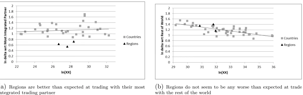
(a) Regions are better than expected at trading with their most integrated trading partner
[image:22.612.60.574.42.203.2](b) Regions do not seem to be any worse than expected at trade with the rest of the world
Figure 4: HRIs with main trading partner and with rest of the world
We investigate this by looking at the three marginal regions of our dataset within a “three
country” framework: the multilateral dataset is aggregated up in each case so that we are
con-sidering the three by three trade matrix involving the region, the rest of its nation, and the rest
of the world. The results of doing this are compared against the equivalent for every country in
the dataset, where the three by three trade matrix now involves the country, its most integrated
trading partner (lowest measured frictions19), and the rest of the world. The results are presented
in Figures 4a and 4b. We can see that the regions have roughly the expected level of trading
frictions with respect to the rest of the world, but lower than expected frictions with their most
integrated trading partner (which is the rest of their nation).
Regions differ from countries in the frictions that they have with their main partner, not in
the frictions that they have with the rest of the world. We do not find that our marginal regions
are systematically less integrated into the global economy than are independent countries of the
same size. It does not seem to be the case that regions are substituting very close trade links
with the rest of their country for slightly closer trade links with all possible partners in the rest
of the world. Instead, the close economic integration across regional borders is on top of normal
trade links with the rest of the world. Therefore the integration benefits of sharing a nation are
apparently additional to the normal integration benefits that countries enjoy within the global
economy.
4.2
Counterfactual exercises
In order to proceed, we need a model in which we can conduct counterfactual analyses. Arkolakis,
Costinot, and Rodr´ıguez-Clare(2012) show that there is a map from trade elasticity,, and home
share, λ, to welfare changes, ∆W, in all “gravity models”, and we have seen that there is a
map from trade flows to the HRI measure of trade frictions implied by such gravity models. We
propose to implement policy experiments by changing the HRI measure of trade frictions. However,
to quantify the welfare change under these policy experiements, we need to know how the trade
flows vary with the HRIs. Unfortunately, as shown in Appendix C, there is no general map from
HRIs to trade flows and a model is needed to provide the necessary structure for a specific set of
HRIs to imply a specific set of counterfactual trade flows and incomes. The welfare formula from
Arkolakis, Costinot, and Rodr´ıguez-Clare (2012) only allows the welfare change to autarky to be
evaluated - since it is only under autarky that we know the value of the counterfactual home share,
λ0 = 100%.
Costinot and Rodr´ıguez-Clare (2014) state that gravity models in which fixed exporting costs
(if any) are paid in the destination country have a stronger equivalence result. In this case,
counterfactual changes in trade flows are exactly the same as in the Armington model. Since this
equivalence result holds across a fairly wide class of common models used in the international trade
literature, it is a natural benchmark to consider.
However, in the data that we use, reported trade flows include intermediate goods,20 and so we
use an extended version of the Armington model with intermediate goods. Arkolakis, Costinot,
and Rodr´ıguez-Clare (2012) note that in “environments with ... tradable intermediate goods ...
our simple welfare formula no longer holds [though] we demonstrate that generalized versions can
easily be derived”. We therefore compute our counterfactual scenarios using our intermediate
goods extended version of the Armington model (see Appendix D)21 in which the welfare formula
20We have found no encompassing regional data reporting trade in value added. Thus, we need to use a model that incorporates trade of intermediates.
is:
∆W =
λ0
λ
(1−1β)
−1 (7)
whereλis the non-traded share of output in the data,λ0 is its value in the counterfactual scenario,
is the trade elasticity (the elasticity of trade flows with respect to trade frictions), and β is the
average share of intermediate goods in total output from Equation (2).
We have detailed regional data, including trade in services, for Scotland, Catalonia, and the
Basque Country as described in Appendix A. We find counterfactual countries for these “marginal
regions” by identifying the least frictional trading partner, the “marginal” country, with respect to
Spain (as a counterfactual for both Catalonia and the Basque Country) and with respect to the UK
(as a counterfactual for Scotland). The independent country that is chosen as the counterfactual
for the corresponding region is the country with the lowest measured HRI with respect to Spain
and the UK. These countries are Portugal and Ireland respectively.
The fact that the counterfactual trading pairs are similar in size to the trading pairs upon
which we are conducting these policy experiments gives further validity to these counterfactual
exercises beyond their intuitive appeal.
The “Average Impact” HRI is the measured HRI for the Region-Rest of Country pair adjusted
by the average border effect. For Catalonia and the Basque Country, we augment the observed
frictions by a factor ASpain obtained from the regional border and Spain coefficients from Table 1,
as well as the 14% trade in services impact from Table 2. For Scotland, we augment the observed
frictions by a factor AU K obtained from the regional border coefficient from Table 1, as well as the
14% trade in services impact from Table 222. Let i be the region, j be the counterfactual, R be
the country of whichi is a part, and r be the rest of this country other than i. Thus, we measure
δir and δjR from trade data, define δjR0 by adjusting δjR for size and distance23 using Table 1, and
22The average value of
lnδ− αdist×dist+αdist2×dist2+αlnXX×lnXX (where the αs are the relevant coefficients from Table 1) for the US internal borders is 4.00, while for the Spanish internal borders it is 3.57. The observed HRI for Scotland is calculated using goods and services data, and so on a consistent basis we add the 14% figure from Table 2 to it to produce an equivalent goods only figure. Then adjusting for distance and size as above gives a figure of 3.94 i.e. internal frictions in the UK look much more like those of the US than they do of Spain, and so we create our “average border effect” counterfactual for Scotland by adjusting by the coefficient on the US border effect only from Table 1.
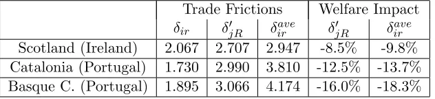
define δaveir =δir×eAR.
Trade Frictions Welfare Impact δir δ0jR δaveir δ0jR δaveir
[image:25.612.150.466.72.144.2]Scotland (Ireland) 2.067 2.707 2.947 -8.5% -9.8% Catalonia (Portugal) 1.730 2.990 3.810 -12.5% -13.7% Basque C. (Portugal) 1.895 3.066 4.174 -16.0% -18.3%
Table 3: Imposing HRIs on regions, with trade elasticity =−3.5
Table 3 shows the measured HRIs for the marginal regions with respect to the rest of the
country of which they are part, the HRIs imposed on these pairs as policy experiments, and the
welfare impact on the marginal regions of performing these policy experiements24.
Notice that the frictions of our“marginal country” counterfactuals are lower than those implied
by an econometric exercise that produces average effects. This is the sense in which our exercise
corrects the selection bias. It would not be reasonable to expect that after a hypothetical Scottish
independence, that the trade frictions between Scotland and England were to become as large as
the ones that the UK has with the average of its other trading partners. The welfare impacts based
on the counterfactual marginal countries are consequently lower than the impact of imposing the
average difference between country and regional frictions.
We rationalise this variation in the impact of the “marginal region” - “marginal country”
dif-share an official language, so Ireland has a common language with the UK, but Portugal does not have a common language with Spain. Regional pairs are deemed always to have a common language (so the assumption is that sufficient Spanish is spoken in Catalonia and the Basque Country for them to share a common language with Spain despite both having local languages. This is a reasonable coding of the data, but strictly following this coding, we would claim that part of the difference between the Portuguese and the Catalonian or Basque frictions was a language effect. We believe that this reading of the relative language frictions in the Catalonia/Basque-Portugal case is incorrect. This is because the business community and professional classes in Portugal can speak Spanish. Designating both cases as positively having a common language designation is therefore reasonable. Modifying one data point in the cross country dataset may not be appropriate - either investigate the data closely in each case or algorithmically code; but sense should be applied when conducting three detailed examples. Note that the purpose of this exercise is to estimate the value of integration directly induced by political integration. It is of course the case that political integration has indirect effects like language homogenization, and perhaps Catalonia and the Basque Country both have a high propensity to cease to have a common language with the rest of Spain if there were to be no political integration in future. In Catalonia, for instance, all education from pre-school to university is given only and exclusively in Catalan, irrespectively of parental language. Moreover there are many voices of the pro-independent movement advocating for Catalan being the solely official language of an independent Catalonia. In the Basque country it is not 100% of the education, but is the large majority in spite of the Basque language being largely minoritarian only one generation ago. In any case, all this is a matter of conjecture (for example it might have been expected that Ireland, upon independence in 1922, would make strong moves away from sharing a common language with the UK and towards being a solely Gaelic speaking country, but this has not happened) and is in any case not the issue we seek to investigate or quantify.
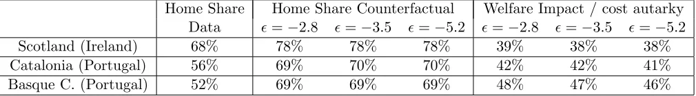
Home Share Home Share Counterfactual Welfare Impact / cost autarky Data =−2.8 =−3.5 =−5.2 =−2.8 =−3.5 =−5.2
Scotland (Ireland) 68% 78% 78% 78% 39% 38% 38%
[image:26.612.57.562.45.115.2]Catalonia (Portugal) 56% 69% 70% 70% 42% 42% 41% Basque C. (Portugal) 52% 69% 69% 69% 48% 47% 46%
Table 4: Welfare changes as a proportion of overall gains from trade are insensitive to changes in the trade elasticity
ference across countries as another point in favour of our proposed method: not only does this
method do as good a job as we are able to do in dealing with this selection bias, it also controls
in some respects for institutional details and country fixed effects. For instance, the fact that the
integration benefit to Spanish regions in being part of Spain is seen to be greater than that of
Scotland in being part of the UK is because Spanish regions seem to be much more integrated into
Spain than Scotland is into the UK.
As well as being sensitive to the value chosen for the trade elasticity, there does not seem to
be much common ground between the welfare figures in Table 3. However, in Table 4 we express
the results of imposing the marginal country friction, δjR, as a counterfactual home share of trade
in GDP, and the welfare loss as a share of the total welfare loss on autarky, for a range of values
of the trade elasticity. We see that the results are remarkably stable. Varying the trade elasticity
makes trade more or less important for welfare, but it is always the case that the gains from trade
associated with sharing a state are a fraction of between a third and a half of the total value of
gains from trade relative to autarky.
This insensitivity of the results to changes in the trade elasticity is implied by insensitivity
of trade flows to the elasticity as described by Section V of Anderson and van Wincoop (2003).
Changing the trade elasticity will change the trade impact of a given change in frictions, or the
welfare impact of a given change in trade. However, conditioning on a counterfactual which is
based on an observation in the data means that different trade elasticities imply different changes
in frictions such that the implied change in trade flows is not greatly affected. Further, whilst the
welfare impact of this implied trade flow change is a strong function of the trade elasticity, it is a
Figure 5: Scottish real income as a function of the trade friction with the rest of the UK.
Imposing measured Scot-rUK frictions implies no change in Scottish income relative to the data. Note that infinite frictions with the rest of the UK is not an autarkic Scotland, frictions with the rest of the world are as measured in the data.
4.3
The incentive to integrate
Finally for this section, we note that income is a convex function of bilateral frictions. Figure 5
shows the level of GDP implied by the model for Scotland as a function of log frictions with the
rest of the UK, relative to the GDP that it has with current frictions. An intuition behind this
convex shape is that it must clearly asymptote to a horizontal line as frictions get very large and
you approach zero bilateral trade: the change from nearly infinite frictions to very large but not
so large frictions will not change trade patterns much once you are not trading at all. Conversely,
the change from medium to small frictions may have a large impact on trade patterns and hence
income.
When two entities are closely integrated (due to high affinities, say) the marginal benefit of
further integration (via political union, say) is larger than it is for entities which are not so
closely integrated (with lower affinities). This supports a selection mechanism whereby pairs with
otherwise lower frictions have a greater incentive to form a unified country than those pairs with
higher frictions. Trade models, in the general class of gravity models, imply greater integration
As an example, in Figure 5 we plot the log frictions that Ireland has with the UK, that Portugal
has with Spain, and the impact that imposing these frictions has on Scottish income. Suppose that
political integration is associated with a reduction in log frictions of sizeI = 0.1. Then, as can be
seen, the income gain, +2.4%, is higher if we start at the less frictional Ireland-UK position, than
if we start at the more frictional Portugal-Spain position, in which case it is +1.6%.
This lends additional support to the proposition that there will be selection into state sharing
and that econometric estimates of the average difference between regional and international borders
is not appropriate for determining the value of the economic integration generated by political
integration.
5
EU Integration and Brexit
In this section we look at the degree of integration that the EU provides, the potential costs of
losing such integration and the potential benefits of furthering that integration.
We start by performing exercises similar to the ones of the previous section, the difference is
that instead of looking at the creation of hypothetical internal borders within countries of the EU,
we look at the effects of a hypothetical departure from the EU. Or perhaps not that hypothetical,
as the UK voted to leave the European Union and is set to formally do so during 2019.
One could argue that augmenting the frictions between the UK and the rest of the EU by the
average impact estimated in the econometric exercise of Section 2, will overestimate the effects of
Brexit by the same reasons that we exposed in section 3: Britain has belonged to the EU for 45
years because of the large degree of affinities with the rest of EU countries, and those affinities are
not likely to disappear as a consequence of Brexit. We consider a set of counterfactual scenarios
to inform on the potential costs of Brexit.
We then consider the gains provided by the existence of the EU to its members, and what
would be the costs of the dissolution of the EU.
Finally, and for the shake of completeness, we revisit the possibility of independence for Scotland
δ Country EU δ Country EU 4.229 LUX 1 4.520 PRT 1 4.242 HUN 1 4.521 LVA 1 4.247 MLT 1 4.525 CYP 1 4.290 BEL 1 4.538 FIN 1 4.298 CZE 1 4.550 ITA 1 4.307 SVK 1 4.555 ESP 1 4.313 NLD 1 4.566 GBR 1 4.318 IRL 1 4.640 TUR 0 4.364 DEU 1 4.695 GRC 1 4.369 SVN 1 4.746 RUS 0 4.371 AUT 1 4.944 TWN 0 4.387 EST 1 4.968 KOR 0 4.402 POL 1 4.988 USA 0 4.423 LTU 1 5.006 CAN 0 4.457 DNK 1 5.056 MEX 0 4.463 CHE 0 5.101 CHN 0 4.469 BGR 1 5.101 BRA 0 4.471 SWE 1 5.122 IND 0 4.491 FRA 1 5.137 AUS 0 4.505 ROU 1 5.187 JPN 0 4.508 NOR 0 5.193 IDN 0 4.512 HRV 1
Table 5: Residual Frictions with the EU after controlling for size of both parties. Residuals frictions with the rest of the Eu if the country belongs to the EU. Residuals frictions given by lnδ−αlnXX×lnXX, whereαlnXX is the coefficient on log (XiXj) from Table 1.
5.1
Brexit Scenarios
A difficulty in trying to make reasonable counterfactuals for the effects of Britain leaving the UK
is the degree of uncertainty on the eventual arrangement. The costs are unlikely to be the same for
staying within the single market (in an EEA type arrangement such as that of Norway) or having
extensive bilateral arrangements that amount to the same (as Switzerland does), as to having the
same frictions that two good neighbors who are both members of the WTO would be expected to
have. In order to clarify matters we produce a set of possible scenarios, measure their impact, and
let the reader use their own criteria for evaluating how reasonable each of these counterfactuals
are.
In Table 5 we order countries by their measured frictions with the EU, once corrected by size.
If the country is a member of the EU, we report its frictions with the rest of the EU. There are two
things to note in this table. First, notice that the UK is amongst the less integrated countries with
the rest of the UK, in the sense than the implied frictions with the rest of the EU are larger than
for all other countries of the EU except Greece. Second, the non EU countries with the smallest
frictions to the EU are Switzerland, Norway, Turkey and Russia (in that order).
Mg region⇒Mg country δir ⇒δ0jR Welfare Change
[image:30.612.159.453.43.143.2]Austria ⇒ Switzerland 2.654⇒2.852 −2.6% Sweden ⇒Norway 2.862⇒3.032 −1.5% Poland⇒ Russia 2.649⇒3.290 −5.4% Bulgaria⇒ Russia 3.596⇒3.593 +0.0% Romania ⇒ Russia 3.278⇒3.474 −1.5% Greece⇒ Turkey 3.988⇒3.384 +3.3%
Table 6: Some Hypothetical exercises within the EU. Implied effect on GDP of the “marginal region” of substituting the frictions with the rest of the EU for the frictions that the counterfactual country (“marginal country”) has with the EU.
the type that we performed in the previous section. Here we define “marginal countries” as non
EU members highly integrated with the EU, and “marginal regions” as the EU countries which
are their most natural counterparts. Notice that Austria “becoming like” Switzerland or Sweden
“becoming like” Norway have relatively small (albeit not insignificant) effects on GDP (of course,
they have larger effects on the size of trade flows with the EU). Poland “becoming like” Russia has
much larger negative consequential effects. The most surprising case is Greece “becoming like”
Turkey, as Turkey trades with more ease with the EU than Greece does. We are skeptical about
this last result, as it might be related to the specific economic circumstances of Greece since 2010,
and in what follows we will ignore comparisons with Greece. In any case, it is informative on the
fact that as countries go, Turkey is relatively well integrated into the EU economy.
In table 7 we report the value of the frictions between “marginal regions and “marginal
coun-tries” in the European context. For Switzerland the natural choice is Austria, and for Norway
it is Sweden. It is not clear what is the natural “Marginal Region” counterpart for Turkey so we
drop this example. The best counterparts for Russia are probably Poland, Bulgaria, or Romania.
Notice that the average differences in log frictions, 0.073625is much lower than the average effect of
the EU on log frictions, which is 0.1444 from Table 1. This is consistent with endogenous selection
into the EU, and suggests that to imply an increase of frictions to be equal to the average effect
of the EU on frictions as a consequence of Brexit could overestimate its effects, as discussed in
section 3.
Thus, we call an increase in the log of EU vs other country frictions of 0.0736, the “causative”
Marginal Region Marginal Country log difference Austria vs Switzerland 2.654 2.852 0.0720
Sweden vs Norway 2.862 3.032 0.0575 Poland vs Russia 2.649 3.290 0.2165 Bulgaria vs Russia 3.596 3.593 -0.0007 Romania vs Russia 3.278 3.474 0.0579
[image:31.612.87.477.44.149.2]Average 0.0736
Table 7: Frictions with the EU of selected countries along with the frictions with the rest of the EU of selected counterparts.
Counterfactual δU K−EU ∆ of logδ δ0U K−EU Welfare Change
“Causative effect” 2.668 0.0736 2.871 -1.0%
“Average effect” 2.668 0.1444 3.082 -1.7%
Table 8: Counterfactual causative and average effects of Brexit. Implied effect on GDP of the UK of increasing (log of) frictions with the EU by 0.0736 (“causative effect”) and 0.1444 (average effect).
effect of the EU on trade frictions. We compare it with the“average” effect of the EU which is the
increase of 0.1444 obtained in Table 1. In Table 8 we show that the“causative” effect of increasing
δU K−EU by the average increase between“marginal regions and countries” in the european context
is a fall of UK GDP of 1.0%, compared with a 1.7% fall as suggested by the average effect.
Notice that the implied “causative” increase in the frictions does not take into account any of
the specificities of the relationship between the UK and the EU. In particular it does not account
for the fact that the UK is a large supplier of financial services to the rest of the Union. Not
only has the UK the largest financial sector share in GDP of all the G7 countries (and more than
twice Germany’s share), but the contribution of UK financial services exports to GDP is also the
highest. This is a sector very sensitive to regulation, and the new political realities in Europe as
a consequence of the UK not having political representation in the Union, open the posibility of
regulatory changes likely to decrease the relative advantage that the UK has now in the sector.
We have seen in section 2.3 that trade in services is typically much more home-biased than goods
trade. It is likely to be the case that this is also the case across the EU border, particularly given
that the political sphere for regulation in those matters lies in Brussels more than in country states.
It seems reasonable to expect regulatory changes making it more difficult for the UK to export
Mg region⇒Mg country δir ⇒δjR0 Welfare Change
[image:32.612.133.428.43.117.2]UK⇒ USA 2.668⇒2.905 −1.1% UK ⇒ Canada 2.668⇒3.674 −2.9% UK⇒ Australia 2.668⇒4.247 −3.5% UK ⇒Russia 2.668⇒3.024 −1.5%
Table 9: Counterfactuals for the UK outside Europe. Frictions of the counterfactual “Marginal Country” are corrected by size, language and distance.
interests are not accounted for in the EU political process. To properly account for those facts lies
beyond the scope of this paper, but those realities should be taken into account when considering
the possible consequences of Brexit.
An alternative, and perhaps more natural, counterfactual for the UK after Brexit are non
Eu-ropean countries that share many cultural, social and political similarities with the UK. Countries
like Canada, USA or Australia. A further natural counterfactual is Russia since post-Brexit, the
UK and Russia will be the two large, culturally European, countries that border the EU. In Table
9 we present the results of the exercise of substituting the frictions that the UK has with the rest
of the union by the frictions that USA, Canada, Australia and Russia have with the EU (after
controlling for size and distance). The effects on UK’s GDP range from decreases of around 1.1%
(if the countarfactual is the USA) to 3.5% (if it is Australia).26
In Figure 6 we summarise these results and show how the welfare impact upon the UK of Brexit
depends on the frictions that the UK may have with the rest of the EU. Not surprisingly it is a
similar to the figure in section 4.3, larger frictions, less trade, worse outcomes, and the gains are
larger the closer you are. There is a difference in magnitudes relative to Figure 4.3 though, since the
Scottish economy is much smaller than the UK’s and it depends much more upon trade (largely
with the rest of the UK). In Figure 6 we mark hypothetical values of δ and the corresponding
welfare imapct upon the UK. The hypothetical frictions that we mark are (1) the frictions that
the UK has currently with the EU. If these were to be the frictions after Brexit (i.e., no change
at all in frictions), there would be of course no change in welfare. (2) The frictions resulting from
adding to the UK-EU frictions, the “causative” effect described above, and the “average” effect
of the EU from Table 1. These result in a loss of about 1.0% and 1.7% of GDP respectively. And