Two-dimensional implementation of the coarsening method for linear peridynamics

Received: 12 January 2019 Accepted: 19 March 2019 Published: 03 April 2019 http://www.aimspress.com/journal/Materials

Research article

Two-dimensional implementation of the coarsening method for linear

peridynamics

Yakubu Galadima, Erkan Oterkus* and Selda Oterkus

Department of Naval Architecture, Ocean and Marine Engineering, University of Strathclyde, 100 Montrose Street, Glasgow G4 0LZ, UK

* Correspondence: Email: [email protected]; Tel: +447714703872.

Abstract: Peridynamic theory was introduced to overcome the limitations of classical continuum mechanics (CCM) in handling discontinuous material response. However, for certain problems, it is computationally expensive with respect to CCM based approaches. To reduce the computational time, a coarsening method was developed and its capabilities were demonstrated for one-dimensional structures by substituting a detailed model with a surrogate model with fewer degrees of freedom. The objective of this study is to extend the application of coarsening method for linear peridynamics for two-dimensional analysis. Moreover, the existing one-dimensional coarsening method was further explored by considering various different micromodulus functions. The numerical results demonstrated that coarsening approach has a potential to reduce the computational time with high accuracy for both one-dimensional and two-dimensional problems.

Keywords: peridynamics; coarsening; non-local; numerical; composite

1. Introduction

using the same field equation as in the continuous case. Another feature of the Peridynamic formulation is that it is a nonlocal theory that incorporates the concept of long-range forces by allowing interaction of particles located at a finite distance from each other through a pairwise force field.

The peridynamic theory has extensively been investigated and is shown to have capabilities of modelling a wide range of engineering problems [2–10]. However, for certain problems, it suffers from the disadvantage of being computationally more expensive compared to the classical continuum theory which is attributable to its nonlocal formulation. In an effort to mitigate against this issue, researchers have proposed a number of multiscale modelling techniques. An adaptive refinement method was proposed in [11] for bond-based peridynamic problems involving a variable horizon. A peridynamic-based framework for hierarchical multiscale modelling was proposed in [12] that couples molecular dynamics and peridynamics. These techniques allow coupling of models at different scales for effective inter-scale information transfer. A coarsening method was also proposed in [13]. The key idea of the coarsening method is to obtain accurate results by solving a reduced order model. The reduction in the order of model is achieved by substituting a detailed model with a surrogate model with fewer degrees of freedom. The objective of this study is to extend the application of a coarsening method for linear peridynamics proposed in [13] for two-dimensional analysis. Moreover, the existing one-dimensional coarsening method was further explored by considering different micromodulus functions other than that considered in [14].

2. Peridynamics

Recalling from the classical continuum theory, the equation of motion of a medium arising from conservation of momentum is as follows:

(1)

where is the mass density of the medium, is the stress tensor, is a vector of body force density, is the acceleration vector field of the material point within the medium at time . The key challenge in using Eq 1 to model discontinuous system behaviour is the presence of the divergence operator, which implies the existence of the spatial derivative of the stress field and consequently the displacement field within the domain of interest. However, since these field variables are not continuous over features such as crack tip and crack surfaces, the derivatives in such instance are undefined. In the peridynamic formulation, the equation of motion was casted such that the integral operators replaced the derivatives on the right hand side of Eq 1. A “bond-based” peridynamic equation of motion was originally proposed by Silling [1] as

₍₂₎

where is the displacement vector field, is the neighbourhood of the particle located at point

2.1. Micromodulus function for linear peridynamics

If we assume a linear material behaviour, then the pairwise force function [1] takes the form

(3)

where is a tensor valued function called the micromodulus function given by

(4)

is the relative position of the particles in the reference configuration, and is their relative displacement. The peridynamic equation of motion (Eq 2) therefore specialises to

₍₅₎

The micromodulus function is required to satisfy certain properties [1]. Moreover, the range of admissible functions that can be used is extensive [14]. However, only a few of them will be discussed here.

The first sets of examples of the micromodulus functions to be given belong to a class of materials called microelastic materials. A peridynamic material is said to be microelastic if the pairwise force function, , is derived from a scalar micropotential, :

(6)

The micropotential, is the energy of a single bond and represents a local strain energy density [2] which is given by

(7)

where the stretch, s can be defined as

(8)

From Eqs 7 and 8, Eq 6 becomes

(9)

where is a function that is characteristic of the material and is called the bond constant. Differentiating Eq 9 with respect to and assuming small displacements yields

for two-dimensional configurations. For one-dimensional configurations, Eq 10 specialises to

(11)

In order to determine the bond constants for microelastic materials, the strain energy density of a given point can be defined [2] as

(12)

2.1.1. One-dimensional micromodulus

Let be the radius of the influence domain or horizon that is characteristic of the material. Then, using Eq 7 and assuming a one-dimensional problem, the peridynamic strain energy density of a material point becomes

(13)

If we assume to be independent of bond length, i.e., , then Eq 13 can be written for constant stretch for all bonds as

(14)

For the same condition, the strain energy density from classical continuum theory can be written as

(15)

Equating Eqs 14 and 15 yields

(16)

Hence, the micromodulus function for this material is

(17)

(18)

Equating Eq 18 with Eq 15 gives

(19)

The micromodulus function in this case is

(20)

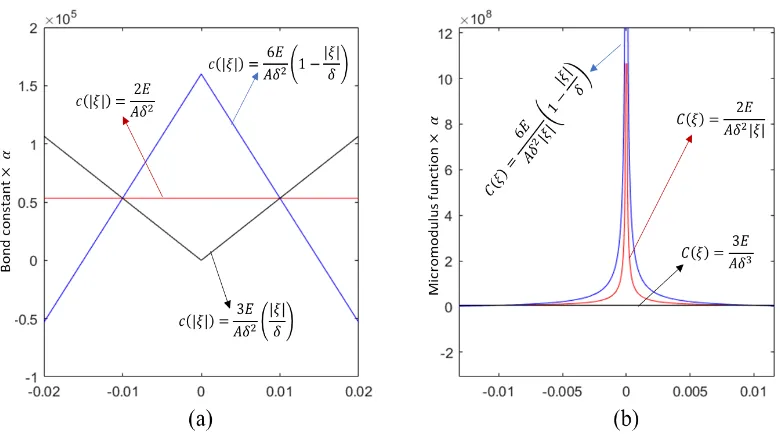
In the case where the dependency of is in the form of an inverted triangular profile [3], in which case, bonds closer to the principal point are softer than bonds further away from it, such that,

for bonds within the horizon. In this case, Eq 13 becomes

(21)

Equating Eq 21 with Eq 15 gives

(22)

The micromodulus function for this scenario then becomes

(23)

Figure 1. (a) Bond elastic functions, (b) Micromodulus functions as changes. 2.1.2. Two-dimensional micromodulus

In the two-dimensional case, let be the radius of sphere describing the horizon. Then, the two-dimensional equivalence of the micromodulus Eqs 17, 20 and 23 are respectively given as

(24)

(25)

(26)

Notice that Eq 26 unlike its one-dimensional counterpart is not a constant function.

3. Coarsening method

microstructure, without necessarily resolving all microstructural details. This is achieved by a process of successive elimination of points from the medium called coarsening. Each successive coarsening results in a medium with a reduced material points as well as reduced level of geometrical detail. However, the properties of the coarsened medium are determined such that the effects of the excluded material points are implicitly included in the coarsened level simulation. The coarsening formulation presented here is adapted from [14] for the completeness of the paper.

3.1. Peridynamic coarsening formulation

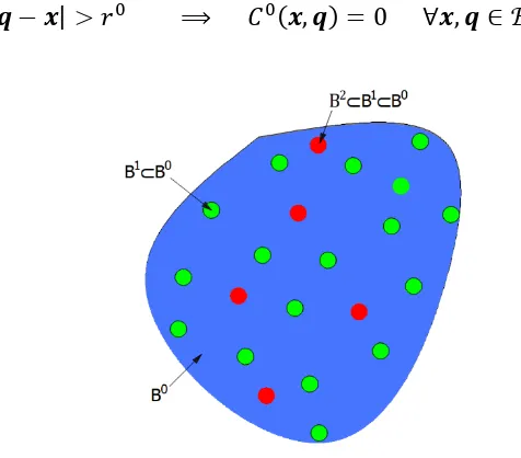
To coarsen a detailed model as proposed in [13], let be a linear elastic peridynamic body as shown in Figure 2. Let be the set of linear admissible displacement fields on , and let

be the micromodulus tensor associated with the material of the body where is the set of all second order tensors. Assume is a positive number that represents the maximum interaction distance for all points in , such that if

(27)

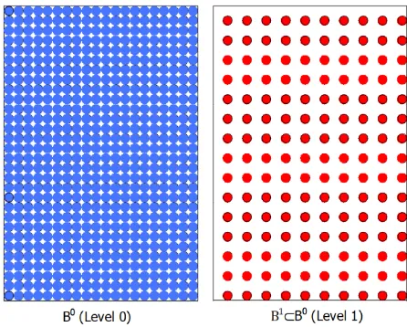
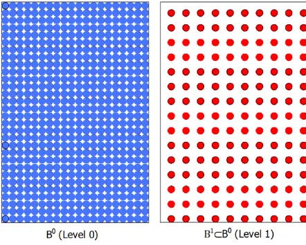
Figure 2. A Peridynamic body showing model levels 0, 1 and 2.

Let , and let represent the set of admissible displacement fields on . and are called level 0 and level 1 body, respectively. The objective of this coarsening process is to express the internal forces acting on in terms of its own displacements only while implicitly accounting for forces points in exert on . To achieve this objective, let be an arbitrary point in and let be a positive number. Let be the closed neighbourhood of in with radius

(28)

Let . Suppose is given and let satisfy the compatibility condition

Outside of , assume that satisfies the equilibrium condition, neglecting interactions between and its exterior:

(30)

where

₍₃₁₎

Also, assume that there is no body force density applied outside

(32)

Further assume that for a given displacement field Eqs 29 and 30 have a unique solution on , and let be the resolvent kernel that generates this solution:

₍₃₃₎

From Eqs 29 and 33, we can infer that

₍₃₄₎

where is the isotropic tensor and is the three dimensional Dirac delta function. For the special case where represents a linear rigid translation of points in through an arbitrary displacement , then all points in will also translate by . Therefore, from Eq 33, we see that

(35)

from which we can obtain the following identity

₍₃₆₎

Subtracting from both sides of Eq 33 and using the identity given in Eq 36, we can obtain

₍₃₇₎

Substituting this result in Eq 31 yields

Reversing the order of integration and rearranging gives

(39)

Recalling that is an arbitrary point in , if we denote the force density in any such choice of by

(40)

Then, from Eqs 39 and 40 we can obtain

₍₄₁₎

where the coarsened micromodulus in level 1 is defined by

₍₄₂₎

Similarly, for any level in the coarsening process, the force density can be obtained from

₍₄₃₎

where the coarsened micromodulus in level m, is defined by

(44)

3.2. Discretization of the coarsening method

To carry out the numerical implementation of the coarsening method described in the preceding section, is discretised into nodes, which for simplicity are taken to have equal volume . Let be the position of node in level . For any nodes and , let

(45)

The coarsened micromodulus is obtained by discretizing Eq 42 as

To evaluate Eq 46, the resolvent kernel needs to be determined. A convenient means of obtaining the kernel function was proposed in [13]. Successive coarsening to higher levels can be achieved by following the same procedure as above, so that for any ,

(47)

To compute the coarsened micromodulus at level for node , the resolvent kernel must be determined. A method was suggested in [13] for determining the resolvent kernel. This method proceeds by creating and merging two sub-systems of equations into a global system of equations. To create such a system, two vectors representing the displacement field in the level body and

representing the displacement field in level body are defined. The relationship between these two displacement fields is formulated as follows:

The displacement fields and for nodes in level body are constrained to satisfy Eq 29:

(48)

The second system of equations is obtained by ensuring that the nodes complementary to nodes in level body satisfy Eqs 30, 31 and 32. Concatenation of these two systems of equations results in a global system of equations that has the following form in one dimension:

(49)

where is the number of nodes in , is the number of nodes in and the diagonal elements are given by

(50)

In shorthand notation, Eq 49 can be written as

(51)

where is square matrix in one-dimension and in two-dimensions. Let

4. Coarsening the micromodulus function

In this section, the coarsened form of various micromodulus functions will be presented. One-dimensional cases will be followed by a two dimensional case.

4.1. Coarsening of one-dimensional micromodulus functions

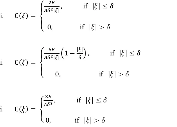
The one-dimensional problem is a homogeneous bar with a length of . The elastic modulus of the material is assumed to be . Three scenarios will be investigated by considering the following micromodulus functions:

i.

(52)

ii.

(53)

iii.

(54)

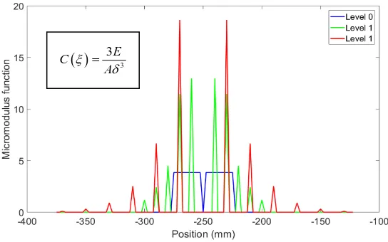
The level 0 horizon is specified as . Note that this same horizon will be used in the coarsened models. The bar is discretized into 400 nodes with spacing Coarsening of the detailed model to the level body is carried out by retaining every fourth node of the level body. Similarly, coarsening of the level body to the level body proceeds by retaining every second node in the level body. Figure 3 shows a schematic representation of the coarsening process. The micromodulus of the detailed model (level 0) as well as the coarsened micromodulus and for the three scenarios are shown in Figures 4 to 6 These curves are characterized by sharp peaks consistent with the fact that the coarsened micromodulus functions are defined only at their respective coarsened regions.

Figure 4. Micromodulus function associated with a uniform bond constant.

Figure 5. Micromodulus function associated with a bond constant function having triangular profile.

Figure 6. Micromodulus function associated with a bond constant function having inverted triangular profile.

  2

2E C

A

   

  3

3E C

A 





  2

6 1

E C

A  

  

 

   

4.2. Coarsening of two-dimensional micromodulus function

The two-dimensional problem is a square plate with a thickness of . Let the elastic modulus of the plate to be and its micromodulus function is given by

(55)

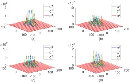
Coarsening is carried out as shown schematically in Figure 7. Every second node in every second row of the level model is retained in the coarsened level model. Similarly, every second node in the second row of level is retained in level body. Figure 8 shows the micromodulus function of the level model as well as the coarsened micromodulus of the level model. It is noticed that the coarsened micromodulus is characterised by sharp peaks which is a reflection of the fact that it is only defined at the coarsened region. Figure 8a shows the response of the material point in the -direction for a displacement of the point in the -direction. Figure 8b shows the response of the material point in the -direction if the

point is displaced in the -direction. Figure 8c shows the response in the -direction of the

point when the point displaces in the -direction. Finally, Figure 8d shows the response of the point in the -direction when the point is displaced in the

-direction.

Figure 8. Coarsening of two-dimensional micromodulus function: (a) interaction (b) interaction (c) interaction, and (d) interaction.

5. Numerical results

This section comprises five numerical experiments to illustrate the application of the coarsening method in solving solid mechanics problems. The systems are assumed to be in a state of static equilibrium and thus an implicit static solution scheme has been utilized. The first three examples focus a one-dimensional bar under tension loading cases for homogeneous and composite materials with and/or without defect. The last two examples demonstrate the capability of the coarsening approach for two dimensional plate problems for isotropic and composite materials.

5.1. One-dimensional homogeneous bar under tension loading

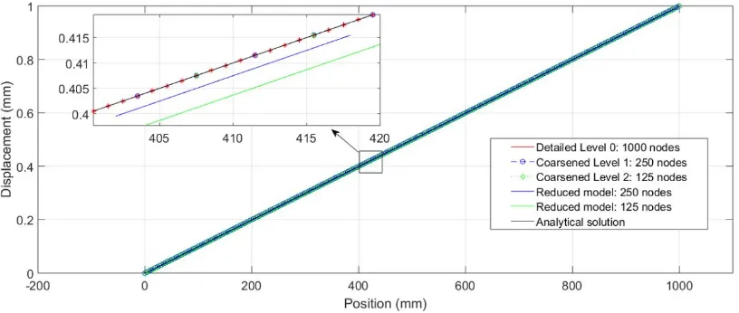
This example is a numerical experiment aimed at illustrating the capability of the coarsening method in capturing the correct bulk behaviour of a system even with reduced degrees of freedom as opposed to if the degrees of freedom were to be reduced without the coarsening process. Consider a bar of length of material having a micromodulus function of the form:

(56)

detailed model (level 0) is discretised into points, so that . The elastic modulus of the material is . Coarsening of the level model to level proceeds by retaining every fourth node in level 0. Level 2 model retains every second node in level model as shown in Figure 3. A body force density of is applied to the rightmost level 2 node, while the third leftmost level 2 node is constrained to have zero displacement. The displacement field associated with the level 0 and coarsened levels 1 and 2 are shown in Figure 9. It is observed that even with reduced degrees of freedom as the detailed model is coarsened into level 1 and subsequently level 2, the displacement fields obtained from all these models are very similar to each other. This would not have been the case if the reduction in degrees of freedom were not achieved through the coarsening process.

The analytical solution based on the classical theory to the axial bar problem is of the form

(57)

where is the distance from the support, is the displacement at point , is the elastic modulus, is the cross sectional area, and is the force applied at the free end of the bar. The result from the analytical model and those from the detail level 0 model as well as the results from coarsened levels 1 and 2 model are almost identical.

To illustrate the need for the coarsening process in achieving model order reduction, the number of nodes was reduced from 1000 to 250 and further to 125 without following the coarsening procedure. As shown in Figure 9, although the results from the coarsened models and the results from the models with reduced number of nodes are very close to each other, coarsened model results agree better with the analytical solution.

Figure 9. Displacement fields for a one-dimensional homogeneous bar under tension loading. 5.2. One-dimensional composite bar under tension loading

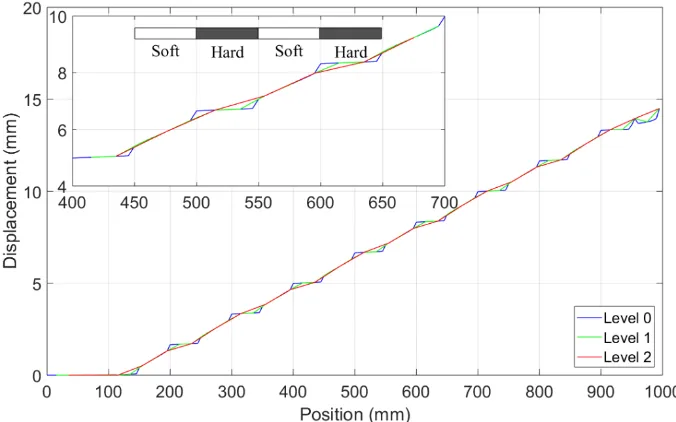
in length. The horizon for both hard and soft section is . The micromodulus of the composite system has the form:

(58)

In other words, bonds with both ends in hard strip have hard properties while bonds with either ends in soft strip have soft properties. The elastic moduli of the hard and soft materials are

and , respectively. The level horizon is specified as . Coarsening from the level to the level body is carried out as shown in Figure 3 by retaining every fourth node of the level body. Similarly, the level body is coarsened to level body by retaining every second node in the level body.

A body force density of is applied to the three rightmost level nodes, while the three leftmost level nodes are constrained to have zero displacement. The computed displacements of coarsened level are shown in Figure 10. As expected, computation from the level revealed the most detailed microstructural information. As the computational regions get coarsened, these microstructural details get smoothed out. However, both detailed and coarsened models have similar global stretch. This demonstrates the fact that the effective properties produced by the coarsening process accurately reflect the bulk properties of the composite.

Figure 10. Displacement fields for levels 0, 1, and 2 for a one-dimensional composite bar under tension loading.

5.3. One-dimensional homogeneous bar with a defect

constitutive model of the bar is given by

(59)

where is a degrading term given by

(60)

The horizon is specified as in the level and the bar is discretised into 200 nodes. The defect is located at the center of the bar as shown in Figure 11. The level contains every third node in the level and similarly, the level contains every third node of the level as shown in Figure 12. Prescribed displacement boundary conditions are applied to the three leftmost and three rightmost level nodes. The values of the prescribed displacements are given by

, where is the coordinate of the node.

Figure 11. One-dimensional homogeneous bar with a defect.

Figure 12. Schematic representation of the coarsening process for example 2.

Figure 13. Coarsened displacement fields in a one-dimensional homogeneous bar with a defect. 5.4. Two-dimensional homogeneous plate under tension loading

This example concerns a two-dimensional homogeneous plate under tension loading. The plate is a square plate. The micromodulus of the plate is chosen as

(61)

The horizon for the level body is specied as . The plate is discretised into 200 points in both and -directions with every point having . The thickness of the plate is . Coarsening of the detailed model is achieved by retaining every second point in the second row as shown schematically in Figure 14.

Two boundary layers each consisting of one grid of points are created; one along the top edge and the other along the bottom edge. At the top boundary layer, every second point of the detailed model is constrained to have zero displacement. A body force density of is applied to every second point in the bottom boundary layer in the detailed model.

The displacement field obtained from solving both a detailed (level ) and the coarsened model (level ) are similar as can be seen from Figure 15 and Figure 16. The displacement profile of a specific grid of points along the -axis and -axis are plotted and shown in Figure 17and Figure 18 respectively. It is observed that both models result in very similar displacement fields.

Figure 15. Profile of -axis displacement field: (a) Detailed (Level ) model and (b) Coarsened (Level ) model.

Figure 17. Profile of displacement field along a grid line of points in the -direction.

Figure 18. Profile of displacement field along a grid line of points in the x-direction. 5.5. Two-dimensional composite plate under tension loading

This example will consider a two-dimensional square plate with periodic microstructure consisting of alternative strips and of hard and soft materials, respectively as shown in Figure 19. Each strip is in length. The horizon for both hard and soft sections is . The micromodulus of the composite system is given by

Figure 19. Discretisation and coarsening of the two-dimensional composite plate.

The horizon is specified as . The plate is discretized into 200 points in both and -directions with every point having . Coarsening of the detailed model and the applied boundary condition is same as that of previous example.

The computed displacement profile along the -direction for the identical boundary condition for the detailed model (level ) and the coarsened model (level ) is shown in Figure 20. It is observed that because the detailed model included more material points, it has been able to resolve more microstructural details than the coarsened models. However, both models have the same global stretch thereby demonstrating that the effective properties obtained using this coarsening method is an accurate representation of the bulk properties of the composite.

6. Computational cost

Determination of computational cost savings arising from coarsening a numerical model will follow from the idea suggested in [1]. Consider a body that is discretized into nodes in the level model. Let be the number of arithmetic operations used by a linear solver to solve the fully coarsened level model, where and are constants ( for Gaussian elimination [1]), and is the total number of nodes in level model. Suppose each level has as many nodes as the previous level, where is a constant, such that

(63)

where is the dimension of the problem (In the example on two dimensional homogeneous plate,

and ).

The computational effort in determining material properties at level from level is proportional to since in doing so, the inverse of the matrix has to be computed. Therefore, for some positive constant , the total arithmetic operations that will be used to coarsen a numerical model and solve the fully coarsened level model can be written as

(64)

It can be concluded from Eq 64 that the computational effort of coarsening up to level in a linear solver for a boundary value problem is reduced by a factor of over the computational effort needed to solve the detailed level model. For a two-dimensional problem such as the example on two-dimensional homogeneous plate, this factor will be . The computational price paid to determine the coarsened properties of the model is less than

which is independent of .

7. Conclusions

computational time and storage required. Another advantage offered by the coarsening method is that the model retains its attributes such as boundary conditions and applied force density after the coarsening process. This is not the case if the model is reduced without going through the coarsening process. In this case, the boundary conditions and applied force density can no longer be identically applied as in the original model.

It is instructive to mention a number of caveats related to this method. This coarsening method is currently valid only for linear and static problems. This limitation is a consequence of assumption made in obtaining Eq 30.

Acknowledgments

The first author is supported by the government of the federal republic of Nigeria through the Petroleum Technology Development Fund (PTDF).

Conflict of interest

The authors declare that there is no conflict of interest regarding the publication of this manuscript.

References

1. Silling SA (2000) Reformulation of elasticity theory for discontinuities and long-range forces. J Mech Phys Solids 48: 175–209.

2. Silling SA, Askari E (2005) A meshfree method based on the peridynamic model of solid mechanics. Comput Struct 83: 1526–1535.

3. Silling SA, Zimmermann M, Abeyaratne R (2003) Deformation of a Peridynamic Bar. J Elasticity 73: 173–190.

4. Ha YD, Bobaru F (2011) Characteristics of dynamic brittle fracture captured with peridynamics. Eng Fract Mech 78: 1156–1168.

5. Parks ML, Lehoucq RB, Plimpton SJ, et al. (2008) Implementing peridynamics within a molecular dynamics code. Comput Phys Commun 179: 777–783.

6. Chen X, Gunzburger M (2011) Continuous and discontinuous finite element methods for a peridynamics model of mechanics. Comput Method Appl M 200: 1237–1250.

7. Ghajari M, Iannucci L, Curtis P (2014) A peridynamic material model for the analysis of dynamic crack propagation in orthotropic media. Comput Method Appl M 276: 431–452.

8. Huang D, Lu GD, Wang CW, et al. (2015) An extended peridynamic approach for deformation and fracture analysis. Eng Fract Mech 141: 196–211.

9. Ha YD, Bobaru F (2010) Studies of dynamic crack propagation and crack branching with peridynamics. Int J Fracture 162: 229–244.

10. Agwai A, Guven I, Madenci E (2011) Predicting crack propagation with peridynamics: a comparative study. Int J Fracture 171: 65.

12. Rahman R, Foster JT, Haque A (2014) A multiscale modeling scheme based on peridynamic theory. Int J Multiscale Com 12: 223–248.

13. Silling SA (2011) A coarsening method for linear peridynamics. Int J Multiscale Com 9: 609–622.

14. Bobaru F, Yang M, Alves LF, et al. (2009) Convergence, adaptive refinement, and scaling in 1D peridynamics. Int J Numer Meth Eng 77: 852–877.