Multi-stage stochastic optimization framework for power generation system planning integrating hybrid uncertainty modelling

Multi-stage stochastic optimization framework for power generation

system planning integrating hybrid uncertainty modelling

Anastasia Ioannou

⁎

, Gulistiani Fuzuli

, Feargal Brennan

, Satya Widya Yudha

, Andrew Angus

Cranfield University, School of Water, Energy and the Environment, Renewable Energy Marine Structures - Centre for Doctoral Training (REMS-CDT), Bedfordshire MK43 0AL, United Kingdom b_{Cranfield University, School of Management, Bedfordshire MK43 0AL, United Kingdom}

c

University of Strathclyde, Department of Naval Architecture, Ocean & Marine Engineering, Glasgow G4 0LZ, United Kingdom

a b s t r a c t

a r t i c l e i n f o

Article history:

Received 5 April 2018

Received in revised form 26 November 2018 Accepted 19 February 2019

Available online 03 March 2019

In this paper, a multi-stage stochastic optimization (MSO) method is proposed for determining the medium to long term power generation mix under uncertain energy demand, fuel prices (coal, natural gas and oil) and, cap-ital cost of renewable energy technologies. The uncertainty of future demand and capcap-ital cost reduction is modelled by means of a scenario tree configuration, whereas the uncertainty of fuel prices is approached through Monte Carlo simulation. Global environmental concerns have rendered essential not only the satisfaction of the energy demand at the least cost but also the mitigation of the environmental impact of the power generation system. As such, renewable energy penetration, CO2,eqmitigation targets, and fuel diversity are imposed through

a set of constraints to align the power generation mix in accordance to the sustainability targets. The model is, then, applied to the Indonesian power generation system context and results are derived for three cases: Least Cost option, Policy Compliance option and Green Energy Policy option. The resulting optimum power generation mixes, discounted total cost, carbon emissions and renewable share are discussed for the planning horizon between 2016 and 2030.

© 2019 The Author(s). Published by Elsevier B.V. This is an open access article under the CC BY license (http://creativecommons.org/licenses/by/4.0/). Keywords:

Multi-stage stochastic optimization Hybrid uncertainty modelling Power generation planning Scenario tree

Monte Carlo simulation Indonesia

1. Introduction

World total electricity generation is expected to grow by 69% from 2012 to 2040 and make up almost a quarter of total energy consumption by 2040 (EIA, 2016). On the other hand, resource depletion and envi-ronmental concerns have forced decision makers to aim not merely to satisfy the increasing demand at the least cost, but also to move towards more sustainable economic development. To this end, many countries have enacted environmental policies to regulate the greenhouse gas (GHG) emissions from power production units using fossil fuels. In 2017, renewable energy sources covered 40% of the increase in primary demand, while net additions of coal-_fired plants are expected to reduce by 55% in the following 20-year horizon, in relation to additions taking place from 2000 up to 2017 (OECD/IEA and IEA, 2017).

Although renewable energy technologies can achieve a reduction in total GHG emissions from power production, their ability to satisfy demand largely depends on the renewable resource potential of the region. Intermittent renewables can provide a certain amount of elec-tricity but are not effective as standalone technologies to provide baseload power. Power generation planning seeks to design the optimal power generation mix by optimizing a performance indicator (such as

minimizing the energy system cost), while at the same time satisfying a set of conditions related, for example, to the security of supply, the limitation of resources, the energy diversity, the environmental impact as well as the renewable technology capacity factors and the evolution of their costs. It is, hence, a challenging undertaking requiring the exam-ination of numerous, often interrelated, aspects.

Mathematical programming is an appropriate method for determin-ing optimal electric power generation systems that will minimize the overall cost (or other objective functions) while satisfying a set of under-lying conditions. Conventional energy planning is performed based on a deterministic projection of demand, capital cost of different generation technologies, fuel prices, etc., assuming that all variables are certain and remain unchanged throughout the planning horizon (Koltsaklis et al., 2014). However, some of the future forecasts, such as demand growth, fuel price and renewable energy cost, are susceptible to change in the fu-ture, making the planning solution invalid when those variables deviate from the forecasted values (Thangavelu et al., 2015).

The present work proposes a linear multi-stage stochastic optimiza-tion (MSO) model that determines the medium-to-long term optimal electricity generation mix, taking into consideration the uncertainty in electricity demand, capital cost reduction for renewable technologies and fuel prices along the planning horizon. In this work, the uncertainties are modelled through a hybrid method combining the Scenario Tree (ST) and the Monte Carlo Simulation (MCS) approach. The volatility of fuel ⁎ Corresponding author.

E-mail address:a.ioannou@cranfield.ac.uk(A. Ioannou).

https://doi.org/10.1016/j.eneco.2019.02.013

0140-9883/© 2019 The Author(s). Published by Elsevier B.V. This is an open access article under the CC BY license (http://creativecommons.org/licenses/by/4.0/). Contents lists available atScienceDirect

Energy Economics

prices (natural gas, oil and coal) was modelled through MCS, while the associated uncertainty in electricity demand growth and capital cost re-duction for renewable technologies was addressed by applying a_finite number of possible weighted scenarios. Applying the MCS to fuel prices enables the extension of the possibilistic (scenario tree) uncertainty modelling approach to a stochastic one, allowing for certain random variables to be represented through continuous probability density func-tions, leading to a more realistic representation of fuel price uncertainty, based on collected historical data rather than assigning a degree of belief to possible scenarios. As such, novelty of this work lies in developing the hybrid uncertainty modelling approach within the stochastic optimiza-tion framework, as well as in the use of updated input data used to perform the optimization of the Indonesian power generation mix. Fur-thermore, we present results for a number of Planning Options (POs) outlined inSection 6to derive useful insights on the response of the sys-tem under different sets of constraints.

Data were collected from online databases, official reports, as well as communication with people from the Ministry of Energy and Mineral Resources of Indonesia, with the aim to derive optimal power genera-tion mixes and addigenera-tional capacity to be built in each period across a timeframe from 2016 to 2030 to satisfy electricity demand while

ful-filling environmental concerns, renewable penetration and energy diversity targets in this case study.

The remainder of this paper is structured as follows:Section 2 pre-sents existing literature dealing with the optimization of the energy mix under uncertainty. The optimization problem is defined inSection 3; Section 4presents the mathematical formulation of the MSO problem outlining its objective function and constraints. Next, inSection 5, the Indonesian energy context is presented, whileSection 6describes the results derived from the application of the MSO method to the baseline case and subsequently to a number of defined POs. Then, inSection 7 re-sults are further discussed and_finally,Section 8draws the main conclu-sions of this work.

2. Literature review on the optimisation of the energy mix under uncertainty

A number of authors have undertaken studies related to the deter-mination of the optimal energy mix at a national (Thangavelu et al., 2015;Prebeg et al., 2016;Ozcan et al., 2014;Ioannou et al., 2017; Costa et al., 2017;Bakirtzis et al., 2012), regional (Koltsaklis et al., 2014;Cheng et al., 2015;Li et al., 2010;Li et al., 2014;Cabello et al., 2014) or even at building (Cano et al., 2016) level. Most studies use the minimization of the power generation system cost as the objective function, which most frequently includes the investment cost of new generating technology, the fuel price, thefixed and variable operating costs. Other costs considered in literature are: salvage and dismantling costs (Cabello et al., 2014;Aghaei et al., 2013), emissions costs (Ahn et al., 2015;Georgiou, 2016;Hu, 2014;Hu et al., 2013), cost of electricity not supplied (Delgado et al., 2011;Feng and Ryan, 2013;Jeppesen et al., 2016), imports of fuel and electricity (Koltsaklis et al., 2014;Georgiou, 2016;Hu, 2014;Hu et al., 2013), cost of carbon capture and storage units (Jeppesen et al., 2016), cost of transmission (Koltsaklis et al., 2014;Zakerinia and Torabi, 2010) and cost of storage (Zakerinia and Torabi, 2010;Krukanont and Tezuka, 2007).

Many works have been established to develop optimization models that incorporate uncertain inputs in the energy generation planning (Ioannou et al., 2017). The MSO method has been widely used to model the uncertainty of selected variables with specific probabilities by means of a multi-period scenario tree. The fundamental concept of MSO is recourse, allowing corrective actions to be implemented in each stage based on the corresponding uncertainty realized so far (Li et al., 2010). In thefirst stage, a decision has to be made“here and now”before perceiving uncertainty, then in the next stage the decision is made after realizing the uncertainty values (Feng and Ryan, 2013;

Krukanont and Tezuka, 2007). For example, the energy mix for period t+ 1 can be decided only after realizing the energy demand at periodt. Li et al. formulated a multi-stage interval-stochastic energy model using integer linear programming for supporting electric power system planning under uncertainty of power demand (Li and Huang, 2012). Through a multi-stage stochastic non-linear programming model, Thangavelu et al. suggested the inclusion of uncertainty in demand, fuel price and technology cost by assigning scenarios to each variable (Thangavelu et al., 2015). Krukanont and Tezuka considered the uncer-tainty of energy demand, plant operating availability and carbon tax rate in developing a two-stage stochastic linear programming optimiza-tion model to analyze the near-term Japanese energy system planning using real data (Krukanont and Tezuka, 2007). Bakirtzis et al. summarised various planning models which incorporated uncertainties, and per-formed a scenario-based mixed-integer linear programming model to illustrate the effect of demand, fuel prices and CO2prices' uncertainties

on planning decisions using real data from the Greek power system (Bakirtzis et al., 2012).

The ST and MCS are two foremost approaches that have been used to represent uncertain parameters in MSO problems. The former approxi-mates continuous distribution into discrete scenarios and performs op-timization at each realization of uncertain parameter weighted with the corresponding discrete probability (Betancourt-Torcat and Almansoori, 2015). The latter portrays input uncertainty by generating random scenarios based on continuous distributions, which can be determined from historical data or expert judgement (Vithayasrichareon and MacGill, 2012). ST has been widely used for structuring stochastic pro-gramming models in power generation system planning (Thangavelu et al., 2015;Li et al., 2010;Cano et al., 2016;Li and Huang, 2012), due to their ability to discretize the vast number of possible outcomes of the uncertain variables (Cano et al., 2016). The ST-based stochastic programming framework is ef_ficient when the optimization problem is convex and the number of decision stages is small (Shapiro, 2006). Nevertheless, a number of scenario reduction techniques (such as back-ward reduction or forback-ward selection) are available to deal with the rapidly growing number of scenarios in a multi-stage stochastic pro-gramming framework (Conejo et al., 2010).

Some previous studies implemented MCS to model uncertainty of key parameters in the power generation mix (Min and Chung, 2013). Tekiner et al. formulated a mixed integer linear programming method to minimize the total weighted three objective functions (total cost, CO2emissions and NOxemissions) and used the MCS technique to

pro-duce 1500 demand scenarios (Tekiner et al., 2010). Betancourt-Torcat and Almansoori used the MCS method to simulate uncertainty associ-ated with natural gas price and developed a multi-period linear model to determine optimal power generation in the United Arab Emirates (Betancourt-Torcat and Almansoori, 2015). Min and Chung also applied the MCS approach to integrate the uncertainty of power demand and fuel prices, and generated a linear model to solve South Korea's long-term power generation mix problem (Min and Chung, 2013). Finally, Piao et al. used the MCS technique to predict power demand and used it as input in a non-linear stochastic optimization model for identifying strategies to improve air quality in Shanghai (Piao et al., 2014).

3. Problem definition

This section outlines the main features of the proposed MSO model for the power generation planning under hybrid uncertainty modelling.

3.1. Problem statement

(NGCC), diesel power, hydro power, geothermal, biomass, wind on-shore, wind offon-shore, solar photovoltaic (PV) and concentrated solar (CSP) power plants. The proposed model and the case study did not consider nuclear energy within the potential power generation technol-ogies because the nuclear energy in Indonesia (which is the case study country) is under continuing debates related to the threats on security in one of the world's most geothermally active nations. The utilization of nuclear energy will be considered only following the optimal utiliza-tion of new energy sources (such as hydrogen, coal bed methane,

lique-fied coal and coal gasification) and renewable energy.

The planning horizon of the problem is divided into a set of time in-tervals,t(with each interval corresponding to a multi-year period) and there is a number of key problem parameters (i.e. electricity demand in-crease, capital cost reduction for renewable technologies and fuel prices for conventional technologies) subject to uncertainty under each inves-tigated scenario,sof time interval,t. The corresponding techno eco-nomic and air emissions data of above energy sources are also given. The PGEP problem aims to determine the combination of energy sources and technologies to meet future electricity demand for each period of the planning horizon under a number of uncertain key parameters.

3.2. Structure of the model

Fig. 1illustrates the structure of the mathematical model, summariz-ing the required input parameters (deterministic and uncertain), the set of constraints, the objective function, the decision variables and the out-put variables. Symbols are summarised in the Nomenclature found in Section 4. Deterministic input parameters include the energy policy tar-gets, as well as the techno economic, resource and technology details. Techno-economic input data of power plants used in the model include capital cost,fixed operation and maintenance (O&M) cost, non-fuel variable O&M cost, carbon emission rate, capacity factor and technical

lifetime of the power plant and were collected both through desktop re-search and through communication with experts. More in specific, data on existing power generation plants of Indonesia, namely the built year, the installed capacity, the decommission time and the capacity factors were obtained following communication with the Ministry of Energy and Natural Resources.

The uncertain parameters comprise the scenario values and proba-bilities of future electricity demand, the capital cost reduction for re-newable technologies and the fuel prices for coal, natural gas and diesel fuels. The incorporation of uncertainties result in the derivation of stochastic planning solutions for power generation mixes.

The constraints that need to be satisfied include the following: (1) meet the future electricity demand at the least cost, both in terms of required installed capacity and net power generation, (2) attain the required renewable penetration targets, (3) restrain CO2,eq

emis-sions within the target set by government regulations, (4) consider annual construction limits for the installation of renewable energy new capacity, (5) the resource potential of the region, and (6) the fuel diversity to manage risk associated with dependency on certain fuel sources or technologies.

Decision variables represent the types and the capacities of the new power plants installed (i.e. the capacity expansion planning) per each time period and scenario. The optimization model, at each time period and scenario, determines the: energy system cost, the existing power generation capacities, the renewable sources contribution to the power generation mix, the power generation cost structure breakdown (capital cost,fixed cost, variable cost, fuel cost and carbon cost) at pres-ent value, the decommissioned power plant facilities that have reached their end of life (decommissioning plan), the required capital cost for the capacity expansion projects, the fuel consumption required by power generation facilities in one year, the annual electricity production from each type of power generation technology, and the GHG emissions

from the power generation system. The mathematical formulation of the optimization problem is presented inSection 4.

3.3. Assumptions of the model

To understand the specifics of the programming approach the fol-lowing well-informed assumptions were considered:

1. Learning curve effects are only applied to the onshore wind and solar PV power plants, whose capital cost is assumed to experience a declining rate through the course of the planning horizon, due to technological development. Capital costs of other technologies were assumed to retain their initial values and future costs were discounted to the present. Furthermore, the capacity factors of all power plant types were assumed to remain constant.

2. The current work integrated the volatility of fuel price into the model for three types of fuels, including coal, natural gas and diesel, while biomass price was assumed to retain a mean value which (similarly to all technologies) is discounted throughout the planning horizon. 3. The PV degradation rate is assumed to remain stable (at 0.8%/year

(Jordan and Kurtz, 2012)) throughout the lifetime of the solar PV power plant. Renewable technologies are assumed to have zero emissions; only emissions during the operation of the conventional power plants are considered and not the lifecycle emissions. 4. It is assumed that, if the system requires capacity expansion at the

beginning of a particular period,tthis expansion project has to be completed by the end of the previous period, denoted astp.

5. The produced electricity (MWh) from conventional energy power plants (coal, natural gas and petroleum-fired power plants) was cal-culated through the fuel consumption rate, which equals the amount of fuel consumed to generate 1 MWh of electricity.Table 1includes the fuel consumption rates used as inputs in the model.

6. The total cost of power generation throughout the planning horizon is discounted to present value with a certain assumption of interest rate.

7. Minimum share of a certain technology can be imposed by setting a minimum contribution of each technology to the energy mix. For example, to manage the risk of intermittency from renewable energy sources policy makers can set the share of coal and gas power at a certain minimum level.

8. The sustainability criteria are fulfilled by means of: the carbon tax, which represents the external cost of environmental impact mitigation; the carbon emission limit, which bounds the amount of CO2,eqemission produced by the power generation sector in one year

and the renewable energy penetration target, which represents the minimum share of power generated from renewable energy sources. 9. Fuel diversity is imposed within an acceptable range by means of enforcing a maximum proportion cap for each technology. The maximum proportion cap can also be used as a tool to restrain an un-desired technology option.

3.4. Uncertainty modelling

In the proposed model, future projection of uncertain variables is represented as a multi-stage ST that grows with both MCS random generated nodes and ST nodes.

1. Energy demand: The uncertainty of peak demand and power con-sumption growth are represented by three ST nodes (low, medium and high) with their assigned probability.

2. Capital cost reduction for renewable technologies: Technology inno-vation is anticipated to gradually reduce the cost of energy of renew-ables. In this study, wind onshore and solar PV are considered to experience a decreasing rate in their capital cost. The uncertainty of the capital cost reduction rate for wind onshore and solar PV are represented by three ST nodes (low, medium and high) with their assigned probability.

3. Fuel Price: The volatility of fuel prices (coal, natural gas and diesel) is represented bynMCS random generated nodes assumed to follow a normal probability distribution function for each fuel type. Normal distribution has been widely used in many stochastic problems (Betancourt-Torcat and Almansoori, 2015;Al-Qahtani et al., 2008); nevertheless, other probability distribution functions were also tested in order to evaluate the effect of statistical uncertainty.

Sections 3.4.1 and 3.4.2present the two distinct uncertainty model-ling approaches.

3.4.1. Monte Carlo simulation

MCS involves the random sampling of the probability distributions of the model's input parameters with the purpose of producing numer-ous random output values. The sampling from each parameter's proba-bility distribution is realized in a way that reproduces the shape of the resulting distribution; hence, the distribution of the output values deriving from the application of the method reflects the joint probability distribution of the outcomes (Vose and Analysis, 2008). It is a standard mathematical procedure, where random inputs are sampled and the output values are recorded for later processing through calculation that a desired event is realized in a number of occasions across the total iterations. Basic steps required to perform MCS are as follows: 1. Definition of the parametric model,y=f(x1,x2,…xq), whereqis the

total number of.

2. Definition of probability distributions for the inputs, number of simulations to accomplish the desired accuracy.

3. Generation of set of random inputsxi1,xi, 2,…,xi,q.

4. Execution of the deterministic model with the set of input parame-ters and recording of output valueyi.

5. Repeat steps 4 and 5 fori= 1 ton.

6. Compilation of the joint probability distribution of the outputsyi.

There are numerous statistical distributions that can be utilized for engineering approximations and random number generations.

In this study the normal probability density distribution is used to model the fuel prices, given by the following equation:

f xð Þ ¼ 1 σpffiffiffiffiffiffi2πexp

−_ðx−μÞ2

=2σ2 _ð1Þ

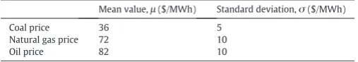
The mean values and standard deviations of the three different types of fuels are summarised inTable 2.

Table 1

Fuel consumption rate used in the model (Source: (Ministry of State Owned Enterprises (SOEs), 2017)).

Fuel type Fuel consumption rate

Coal 0.53 Ton/MWh

Natural gas 8.9 MMBTU/MWh

Petroleum 1.81 Barrel/MWh

Table 2

Mean values and standard deviations of fuel prices of conventional technologies (Source: (Ministry of State Owned Enterprises (SOEs), 2017)).

Mean value,μ($/MWh) Standard deviation,σ($/MWh)

Coal price 36 5

Natural gas price 72 10

3.4.2. Scenario tree approach

A ST is an ensemble of scenarios (or else realizations), s of the future. It is de_fined by a set of nodes,k_∈K, their successors (called children nodes)Bkand their associated probabilities,p(sk). A scenario is a path

from the root node to a leaf node (having no successors) and the prob-ability of scenario, s (denoted asp(ts)) equals the product of probability

of occurrence (joint probability) realized from root node to leaf node p(ts)=∏kϵKp(sk). Each stage of the time horizon,t∈Tis associated to a

set of nodes (representing the different evolutions of the uncertain pa-rameters) forming a set of scenarios. It is a necessary condition, the sum of all probabilities of each scenario within a specific time period to be equal to one,∑(s)p(ts)= 1.

In this work, the uncertainty is modelled by means of a three-stage ST as illustrated inFig. 2. The system covers a time horizon of 3 time pe-riods consisting of 4, 5 and 5 years duration, respectively. The number of nodes and_finite scenarios is determined by the three uncertain vari-ables (electricity demand, capital cost reduction and fuel price). During thefirst time period, both the uncertainty of electricity demand and capital cost reduction are represented by three nodes:_“Low_”,_“Medium_” and“High”with assigned probability valuespL,pMandpH, respectively

(producing 3 · 3 = 32 _{scenarios within the first time period),}

while the uncertainty of fuel prices is represented bynnodes, with 1/nassigned probability each, sampled by means of a MCS process, leading to a total ofn· 32_{scenarios, wherenis the set of random MCS}

samples andtis the number of the stage, as shown inFig. 2.

After reaching the leaf node of each stage's scenarios, the values of the decision variables (new installed capacities of each plant type) of then nodes (representing the uncertainty of fuel prices) are averaged to pro-vide the input value for the next node. Hence, in each stage,n· 32·t

sce-narios are generated. Thefluctuations in the fuel prices were assumed to follow a normal probability distribution, as it is the standard distribution used for many probability problems (Betancourt-Torcat and Almansoori, 2015). MCS generated a random set of fuel prices based on the mean and standard deviation values given inTable 2. It should be highlighted that increasing the sizenof the MCS generated samples can provide more ro-bust results; however, it significantly increases the processing time.

The method can be extended to incorporate other uncertainties; nevertheless, the ones chosen have been widely cited in literature as among the most impactful (Thangavelu et al., 2015; Li et al., 2010;Vespucci et al., 2016;Ji et al., 2015;Vespucci et al., 2014;Kim et al., 2012).

4. Model formulation

The mathematical formulation of the optimization model is pre-sented in this section, starting with the electricity system costs, followed by the constraints and the objective function formulation of the problem.

Nomenclature

The notations of the sets, parameters and variables, along with their measurement units are de_fined in order to introduce the mathematical model:

Sets

p(sD)_{= {0.3,0.5,0.2} Probability of energy demand scenario} p(sC)_{= {0.3,0.5,0.2} Probability of capital cost reduction scenario} pðsFÞ¼ f1

n; ::;1ng Probability of fuel cost volatility scenario

p(s)=p(sD)∙_p(sC)∙_p(sF) _{Probability of occurrence of scenarios s} sC={1, 2,…, 10} Capital cost reduction scenario of new onshore wind

and solar power plants sD= {1,2,3} Energy demand scenario

sF= {1,2, 3} Coal, gas and oil fuel price scenario

s= {sC,sD,sF} Combination of scenarios/realizationssC,sD,sF t= {1, 2,3} Time period

tp Previous time period (years)

τ= {1,2,…,10} Power generation plant: coal: 1, natural gas: 2, oil: 3, hydro: 4, geothermal: 5, biomass: 6, onshore wind: 7, offshore wind: 8, solar PV: 9 and solar CSP: 10 n Number of MCS samples

dv Set of decision variables

k∈K Set of nodes comprising a scenario Parameters

Crateτ CO2,eqemission rate of power generation plant,τ(tons of

CO2/MWh)

CFτ Capacity factor of power generation plant,τ(%)

CLτ Annual construction limit for each technology,τ(MW/year) Ctaxt Carbon tax ($/ton of CO2,eq)

Lfτ Operating life of power generation plant,τ(years)

Lτ Transmission and distribution losses of power generation plant,τ(%)

Maxcapt,τ Maximum proportion of power generation plant,τin energy mix (%) during time period,t

Mincapt,τ Minimum proportion of power generation plant,τin energy mix during time period,t(%)

Oτ Own power use of power generation plant,τ(%)

REpott,τ Renewable energy potential limit of power generation plant,

τduring time period,t(in MW)

REtargett Renewable energy penetration target of power generation

plant,τin energy mix (in %)

VOMτ Non-fuel variable O&M cost of power generation plant,τ

($/MWh)

FOMτ Fixed O&M cost of power generation plant,τ($/kW) RM Supply reserve margin (%)

r Interest rate (%)

Variables

Cemitt(s) CO2,eqemitted per year during time period,tunder scenarios

∈[sC,sD,sF] (ton of CO2,eq/year)

CDt(sD) Power consumption demand power generation plant,τunder

scenariosD(MWh) ECAPEXτ,tp

(sC) _{Capital factor of existing power generation plant,}τ_installed during the previous time period,tpunder scenariosC($/kW) ECt(s) Power generation cost of existing power generation plant,

τduring time period,t($/year)

EICτ(,st) Installed capacity of existing power generation plant,τduring

time period,tunder scenarioss∈[sC,sD,sF] (MW)

EACPt(s) Annualized capital cost of existing power plants during time

period,tand under scenarios∈[sC,sD,sF] ($/year)

ECCt(s) Carbon cost of existing power generation plant,τduring time

period,tand under scenarios($/year)

EFCt(s) Fuel cost of existing power generation plant,τand under

sce-narios($/year)

EFOMt(s) Fixed O&M cost of existing power generation technology, τand under scenarios($/year)

EVOMt(s) Νon-fuel variable O&M cost of existing power generation

technology,τand under scenarios($/year)

ft(s) Total power generation cost discounted to present value

during time period,tand under scenarios($)

FPτ(sF) _{Fuel price of power generation technology,}τ_{and under} sce-nariosf($/MWh)

NACPt(s) Annualized capital cost of new power generation plants, τand under scenarios($/year)

NCAPEXτ,tp

(sC) _{Capital factor of new power plants,}τ_{during time period,} tand under scenariosC($/kW)

NCt(s) Power generation cost of new power plants,τand under

sce-narios($/year)

NICτ(,st) Installed capacity of new power generation plants,τduring

time period,tand under scenarios(MW) PDt(SD) Peak demand (MW)

RICt(SD) Required installed capacity of power generation plant,τ

under scenariosD(MW)

NCCt(s) Carbon cost of new power plants of new power generation

plant,τunder scenarios($/year)

NFCt(s) Fuel cost of new power plants of new power generation plant, τunder scenarios($/year)

NFOMt(s) Fixed O&M cost of new power generation plant,τunder

sce-narios($/year)

NVOMt(s) Νon-fuel variable O&M cost of new power generation plant,τ

under scenarios($/year)

Abbreviations

PGEP Power generation expansion planning PCF Pulverized coal-fired

NGCC Natural gas combined cycle PV Photovoltaic

CSP Concentrated solar power MCS Monte Carlo Simulation ST Scenario Tree

4.1. Generating costs

The total electricity system cost consists of the annualized capital cost, the annualfixed and variable operating (O&M) costs, as well as the fuel and carbon costs of existing and newly installed power plants. The total capital cost is annualized over the lifetime of the power generation plant, while the rest of the costs are measured on a yearly basis. Fixed O&M cost represents the operation and maintenance costs that are not dependent on the power output of the plant, while non-fuel variable O&M cost, non-fuel cost and carbon emission cost vary accord-ing to the energy production of the plant. Solar PV and wind onshore technologies are subject to capital cost reduction over the planning ho-rizon due to assumed technological advancements.

The annualized capital cost of the existing power generation capac-ity is calculated based on the discount rate (r) and the operating life of the power production plant (Lfτ), by means of the following formula:

EACPð Þ_ts ¼ X τ∈ð7;9Þ

X3

sC¼1 EICð ÞsC

τ;t ECAPEX sC

ð Þ τ;tpp

sC

ð Þ

þ X

τ∉ð7;9Þ

EICð Þ_τs_;tECAPEXτ;tp

2 4

3 5

r

1₋ð1þrÞ−Lfτ ∀t¼1:3 ands∈½sD;sC;sF

ð2Þ

where,τdenotes the type of technology, withτ= 1 : 3 representing the conventional technologies andτ= 4 : 10 the renewable energy tech-nologies,EICτ,(ts)stands for the technology'sτtotal installed capacity

(MW) during the time periodt,ECAPEXτ,tp

(sC)_{is the capital cost in the} previous periodtpand the term_1−ð1þr_rÞ−Lf_τ is the amortization factor (Papapetrou et al., 2017), converting the overnight capital expenditure into annual equivalents throughout the power plant's operating life. Accordingly, thefixed O&M cost is calculated as:

EFOMð Þts ¼

X10

τ¼1

EICð Þ_τs_;tFOMτ

∀t¼1:3 ands∈½sD;sC;sF

ð3Þ

where,EFOMt(s)is thefixed O&M cost of installed capacity of existing

power plants per year calculated for each scenario and time period. The non-fuel variable O&M cost per year of existing power plants (EVOMt(s)) is estimated by the following equation:

EVOMð Þts ¼

X10

τ¼1

EICð Þ_τs_;tCFτVOMτ8760

∀t¼1:3 ands∈½sD;sC;sF

ð4Þ

one MWh of power generated technology (τ) while the term 8760 represents the number of hours per year. The fuel cost of existing fuel-powered energy plants (EFCt(s)) is calculated as:

EFCð Þts ¼

X3

τ¼1

Xn

sF¼1 EICð ÞsF

τ;t CFτFP sF ð Þ

τ pð ÞsF 8760

; ∀t¼1:3 ð5Þ

where,FPτ(sF)denotes the fuel price under scenariosF. Finally, the

an-nual carbon cost of existing power plants,ECC(ts)is estimated as

fol-lows:

ECCð Þts ¼Cemit s ð Þ

t Ctaxt; ∀t¼1:3 ands∈½sD;sC;sF ð6Þ where, the mass of CO2,eqemitted per year (Cemitt(s)) is calculated as a

function of the CO2,eq emission rate of power plant technology

(Crateτ) estimated by the following formula:

Cemitð Þts ¼

X3

τ¼1

EICð Þ_τs_;tCFτCrateτ8760

; ∀t¼1:3 ands∈½sD;sC;sF ð7Þ

Above equations are also applied for the new power generation plants. The electricity system cost of new power plants was estimated for every scenario and time period as:

NCð Þts ¼NACP s ð Þ t þNFOM

s ð Þ t þNVOM

s ð Þ t þNFC

s ð Þ t þNCC

s ð Þ

t ð8Þ

NACPð Þ_ts ¼ X τ∈ð7;9Þ

X3

sC¼1

NICð ÞsC τ;t NCAPEX

sC

ð Þ τ;tpp

sC

ð Þ

þ X

τ∉ð7;9Þ

NICð Þ_τs_;tNCAPEXτ;tp

2 4 3 5 r

1−ð1þrÞ−Lf_τ

ð9Þ

NFOMð Þts ¼

X10

τ¼1

NICð Þ_τs_;tFOMτ

ð10Þ

NVOMð Þts ¼

X10

τ¼1

NICð Þ_τs_;tCFτVOMτ8760

ð11Þ

NFCð Þts ¼

X3

τ¼1

Xn

sF¼1 NICð ÞsF

τ;t CFτFPτð ÞsF pð ÞsF 8760

ð12Þ

NCCð Þts ¼

X3

τ¼1

NICð Þ_τs_;tCFτCrateτCtaxt8760

∀t¼1:3 ands∈½sD;sC;sF

ð13Þ

4.2. Constraints

The total installed capacity, namely the existing and new power generation capacity must satisfy the peak demand of the country, PD(tsD)for all demand scenarios,sDand time periods,t. Furthermore,

a reserve margin is taken into account as a buffer to protect against system breakdowns or sudden upsurges in electricity demand. The re-serve margin is defined as the difference between the (required) installed capacity (RIC) and the peak demand divided by the peak demand (Turvey and Anderson, 1977;International Atomic Energy Agency, 1977).

RM¼RIC SD ð Þ t −PD

sD ð Þ t PDð ÞsD

t

; ∀t¼1:3 ð14Þ

Electricity demand is driven by population growth, economic devel-opment and various other factors. However, extensive electricity de-mand estimation is not the focus of the current work. The following

constraint ensures that the installed capacity of existing power plants plus the installed capacity of new power plants are sufficient to meet the expected peak demand plus the reserve margin, hence the required installed capacity after reordering Eq.(14)should satisfy the following inequality:

X10

τ¼1

EICð Þ_τs_;tþNIC s ð Þ

τ;t

≥RICð ÞsD

t ; ∀t¼1:3 ands∈½sD;sC;sF ð15Þ

The net electricity produced by the available power generation facilities is estimated after accounting for the plant's own use of electric-ity (Oτ), the transmission and distribution losses (Lτ). Net electricity must exceed the projected power consumption (CDt(sD)) across all

years between the time periods.

X10

τ¼1

EICð Þ_τs_;tþNIC s ð Þ

τ;t

CF_τð1−ðO_τþL_τÞÞ

h i

≥X3 sD¼1

pð ÞsD _CDð ÞsD t

∀t¼1:3 ands∈½sD;sC;sF

ð16Þ

To satisfy the renewable penetration targets, a minimum renewable energy share in the power generation mix is set to boost renewable energy penetration. This constraint can be varied across the different time periods, with targets set at more ambitious levels in the course of time.

∑10

τ¼4 EICð Þτs;tCFτ

þ∑10

τ¼4 NICð Þτs;tCFτ

∑10

τ¼1 EICð Þτs;t∙CFτ

þ∑10

τ¼1 NICð Þτs;tCFτ

≥REtargett

∀t¼1:3 ands∈½sD;sC;sF

ð17Þ

Subsequently, to enhance the diversity and security of the energy mix, minimum and maximum contributions of each technology can be set. For example, to manage the risk of intermittency from renewable energy sources, policy makers can set the share of coal and gas power at a certain minimum level (Mincapt,τ). This constraint can be applied across all technologies and time periods:

EICð Þ_τs_;tCFτþNICð Þτs;tCFτ

∑10

τ¼1 EICð Þτs;tCFτ

þ∑10

τ¼1 NICð Þτs;tCFτ

≥Mincapt;τ

∀t¼1:3; τ¼1:10 ands∈½sD;sC;sF

ð18Þ

Imposing a maximum proportion constraint, for example on the most cost efficient power generation technologies, forces the model to introduce other less cost efficient technologies in the power generation mix so as to cover the energy demand, rendering the mix more diverse. Fuel diversity can be enforced by policy makers to confine the dependency on a technology or fuel source under a rea-sonable level through setting a maximum proportion cap (Maxcapt,τ) for each technology,τ, and time period,t. Grid stability is another impor-tant factor that should be taken into account. The fact that most renew-able energy technologies cannot be dispatched when required, as they strongly depend on weather conditions, prevents them from being a re-liable base-load solution over a long term period. To this end, the total electricity production from renewable sources can be set not to exceed a maximum proportion.

EICð Þ_τs_;tCF_τþNICð Þ_τs_;tCF_τ ∑10

τ¼1 EICð Þτs;tCFτ

þ∑10

τ¼1 NICð Þτs;tCFτ

≤ Maxcapt;τ

∀t¼1:3;τ¼1:10 ands∈½sD;sC;sF

ð19Þ

The following constraint limits the allowable amount of CO2,eq

and obliging the inclusion of renewable technologies to the mix so as to satisfy the rest of the demand. Different limits can apply at each planning period.

X3

τ¼1

EICð Þ_τs_;tþNIC s ð Þ

τ;t

CFτCrateτ8760

≤Ctargett ∀t¼1:3 ands∈½sD;sC;sF

ð20Þ

The renewable potential expresses the theoretical upper limit of the amount of energy that can be produced from renewable sources over a particular geographic region as estimated by surveys undertaken by ex-perts (Ahn et al., 2015). The following constraint is imposed on renew-able technologies to make sure the power produced from renewrenew-able sources is within the potential capacity of that region or country.

EICð Þ_τs_;tþNIC s ð Þ

τ;t≤REpott;τ

∀t¼1:3; τ∈½4:10ands∈½sD;sC;sF ð21Þ

In this study, the maximum potential (REpott,τ) for hydro, geother-mal, biomass, onshore wind, offshore wind, solar PV and solar CSP are summarised inTable 4.

The annual construction of new renewable energy plants is subject to the availability of labour, manufacturing capacity, area available for construction and social readiness for a particular technology. There is therefore an upper construction limit which remains unchanged across the different time periods.

NICð Þ_τs_;t≤CLτ

∀t¼1:3;τ∈½4:10ands∈½sD;sC;sF ð22Þ

Finally, it should be assured that only non-negative new rated capac-ities can be accepted for every scenario, time period and technology in the solution.

NICð Þ_τs_;t≥0

∀t;s∈½sD;sC;sFandτ¼1:10 ð23Þ

4.3. Objective function

The objective of the optimization problem is to minimize the discounted total cost of the power generation mix (consisting of power plants,τ) for each stage,tand scenario,s(namely, the set of com-binations of scenariossD,sC,sF).The objective cost function (ft(s)) of the

optimization model is presented below:

The set of decision variables (dv) of the problem comprises: the types of new power plants to be installed and their corresponding installed capacities (NICτ(,st)), while other variables determined per

sce-nario and time period include: the probabilities of all scesce-narios (p(s)_),

the cost of existing and new energy system (total and per plant type),

along with their consisting costs (e.g. annualized CAPEX, fuel cost,

fixed O&M cost), the required installed capacities (RICt(SD)), the total

decommissioned capacities, the existing installed capacities (total and per plant type), the new installed capacities (total and per plant type), the total installed capacities (total and per plant type), the forecasted power consumption, as well as the total CO2,eqemission mass and

cost. The proposed optimization model was developed using the constrained solver fmincon of MATLAB R2017a optimization toolbox, based on the interior-point algorithm (Potra and Wright, 2000), while the sequential quadratic programming was also tested (Boggs and Tolle, 1995). The potential of falling into a local minimum in the analysis has been investigated through changing the initial guess of decision var-iables and comparing the results obtained. The different algorithms and initial guesses yielded consistent results.

Following the derivation of the optimal power generation mixes across all scenarios and time periods, boxplots were produced to illustrate the resulting energy mixes, along with the weighted mean proportions of each power plant type, taking into account the scenarios' probabilities.

5. Application to the Indonesian power generation system

In this study, Indonesia's power system's portfolio is used as input for the proposed model. Indonesia's prominence is highlighted by its population of 255 million people (fourth largest in the world) in 2016 (PWC, 2017) and its considerable potential of fossil-fuel and renewable resources. Globally, Indonesia is the largest coal exporter and fourth largest coal producer. The country has an estimated 28 billion tons of coal reserves (accounting for 3.1% of total global reserves (British Petroleum (BP), 2016)). It is the world's tenth largest producer of natu-ral gas and the seventh largest exporter of liquefied natural gas (LNG) (International Energy Agency, 2015).

Indonesia is the largest economy in Southeast Asia and has achieved steady, high growth rates over the last 15 years. Its energy consumption is predicted to grow rapidly as a result of population growth, rapid ur-banisation and rising living standards (International Energy Agency, 2015). Therefore, satisfying demand growth and ensuring the sustain-ability of energy supplies is one of key pillars of Indonesia's economy. In 2016, Indonesia had approximately 59.6 GW installed power plant capacity, generating 290 TWh of electricity (PWC, 2017). Electricity peak load was estimated to reach 32,204 MW in 2017 (Ministry Of Energy and Mineral Resources Republic of Indonesia, 2017). Energy mix is currently comprised by coal (54.69%), gas (25.89%), oil (6.97%) and renewables (12.45%) (Direktorat Jenderal Ketenagalistrikan Kementerian Energy Dan Sumber Daya Mineral, 2017). The Indonesian government seeks to reduce the dependency on fossil fuel by increasing the renewable energy contribution to the power sector by at least 25% by 2030 (Directorate General for Electricity and Energy Utilization, 2015). Additionally, according to the 2014 National Energy Policy (the

“2014 NEP”) of Indonesia, renewable energy should reach at least the 23% of the power generation mix by 2025, while in 2050 the target is to increase renewables share to at least 31% (Government of Indonesia, 2014). As a contingency to the high share of renewable energy in the country's mix, PLN (the company responsible for the ma-jority of Indonesia's energy production) will be required to use another 5.1 GW of gas-fired power plants to meet the resilience requirements of the power generation system (Ministry of Energy and Mineral Resources, 2017). The forecasted power demand growth and base fuel price assumption data were obtained from the National Electricity General Plan (RUKN) draft in 2015. RUKN also specifically sets the minimum reserve margin target (set to 35%), as well as the assumption on own use and transmission losses of the power system in Indonesia (9.48% according to (Ministry Of Energy and Mineral Resources Republic of Indonesia, 2017)). The carbon emission reduction target was set to 26% from the Business As Usual (BAU) value in 2030, as specified in Presidential Decree No. 61 of 2011 on the National Action min

dv f ðsÞ t ¼EC

ðsÞ t þNC

ðsÞ t

¼EACPðtsÞþEFOM ðsÞ t þEVOM

ðsÞ t þEFC

ðsÞ t þECC

ðsÞ t

þNACPðtsÞþNFOM ðsÞ t þNVOM

ðsÞ t þNFC

ðsÞ t þNCC

ðsÞ t

(1)

Subject to

Total installed capacity should satisfy peak demand (15)

Net electricity production should satisfy electricity consumption demand (16)

Renewable energy targets should be fulfilled (17)

Ensure the fuel diversity and energy security of the power generation mix (18)–(19)

Restrain CO2,eqemissions of the power generation mix (20)

Satisfy resource potential limit of the region (21)

Satisfy annual construction limit of the power plants (22)

Plan for Reducing Emissions of Greenhouse Gases in efforts to enforce environmental impact mitigation (Government of Indonesia, 2011). The summary of Indonesia's 2015 initialfleet capacity by generation technology can be found inTable 3.

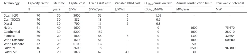
Furthermore, the detailed techno-economic data used as input in the present case study and their references are shown inTable 4. Each technology is characterized by a capacity factor. The capacity factor is defined as the ratio of the actual electricity output during a certain amount of time to the maximum potential electrical output during this period.

Nuclear energy was not considered as an option due to the current lack of political will from the government and the limited support from the public due to safety issues (Hariyadi, 2016). Furthermore, ac-cording to the National Energy Plan of Indonesia (2017), nuclear energy will be considered as the last option, if despite the optimal utilization of new energy and renewable energy sources, the renewable energy target of 23% in total energy consumption is not reached by 2025 (Directorate General for Electricity and Energy Utilization, 2015). As carbon tax has not been implemented in Indonesia yet, the baseline case does not include it in the cost of electricity generation, while the imports and exports of electricity are not taken into account in this case study as the amount of power exchange with neighbouring countries is not significant. The annual construction limits of the renewable energy gen-eration technologies were estimated on the basis of historic annual installed capacities of each technology as well as the renewable energy potential (summarised inTable 4). Under the business-as-usual (BAU) scenario, carbon emissions from the power sector are projected to reach 750 million tons in 2020, 1000 million tons in 2025 and 1250 million tons in 2030 (Asian Development Bank, 2016). Data on costs of power plants differ considerably across literature. To this end, thefinal values considered in the model were derived after retrieving a number of re-cent references (such as the NREL Annual Technology Baseline database (National Renewable Energy Laboratory, 2018)) and calculating their average values.

In addition, the MCS sample size was determined through a conver-gence study, according to which the optimization problem was run with different MCS samples (i.e. for 20, 50, 100, 150, 200 and 500 iterations) and subsequently the resulting total weighted new installed capacities, estimated for each time period, were compared. The minimum number of MCS samples required for the results of the case study to converge was determined 150, i.e. further increase in the sample did not change the solution noticeably but it had an impact on the computational time. The uncertainty of electricity demand and capital cost reduction are represented by three nodes:“Low”,“Medium”and“High”with assigned probability values 0.3, 0.5 and 0.2, respectively adopting the approach of (Thangavelu et al., 2015). For the electricity demand sce-nario, the three possible nodes correspond to demand increase of 5% (low), 8% (medium) and 11% (high) per annum; while the nodes refer-ring to the future values of capital cost for onshore wind and solar PV power plants were retrieved from the National Renewable Energy Laboratory (NREL) Annual Technology Baseline (ATB) 2018 database (National Renewable Energy Laboratory, 2018), which provide trajecto-ries of costs for energy technologies. The time setrajecto-ries values used as input to the model are summarised inAppendix A.

As shown inFig. 2, the number of optimization scenarios for n = 150 were amounted to 1350, 12,150 and 109,350, derived through the com-bination of scenariossC,sD,sFduring thefirst, second and third time

periods, respectively. For each optimization scenario, there are 10 deci-sion variables, standing for the new installed capacities (NICτ(,st)) of the

power plant technologies and 44 constraints.

6. Results

The case study performed capacity expansion planning with 2016 as the base year and three planning stages at years 2020, 2025 and 2035. The stochastic optimization model minimizes the total expected cost of the power generation mix for all three planning stages by considering all possible input scenarios. The proposed model was initially applied to determine the optimal power generation mix under a baseline case. Accordingly, the model was applied under three representative cases calling for: Least Cost option, Policy Compliance option and Green Energy Policy option, which aim to determine the stochastic power generation mix under a set of different policy priorities, modelled in the proposed methodology through adjusting the corresponding constraints' limits.

6.1. Baseline case

Under the baseline case, existing targets for renewable energy con-tribution were considered as input to the model (minimum increase of 16% by 2020, 23% by 2025, and 31% in 2050), the maximum CO2,eq

emissions limit was set according to the BAU scenario for each planning

Table 4

Techno-economic data of power plantsa

.

Technology Capacity factor Life time Capital cost Fixed O&M cost Variable O&M cost CO2,eqemission rate Annual construction limit Renewable potential

% years $/kW $/kW/year $/MWh tCO2,eq/MWh MW/year MW

Coal (PCF) 70 30 3600 33 5 1.09 – –

Gas (NGCC) 70 30 882 18 6 0.6 – –

Diesel 70 30 700 11 6 0.8 – –

Hydro 61 40 4600 75 – 0 1600 75,670

Geothermal 80 30 5200 152 – 0 1000 28,910

Biomass 56 20 4000 58 5 0 1300 32,654

Wind Onshore 35 30 1615 51 – 0 1000 60,600

Wind Offshore 42 25 6100 132 – 0 50

Solar PV 16 25 2600 18 – 0 8500 207,800

Solar CSP 53 20 7872 67 4.1 0 30

a

Techno-economic data derived from the average value of various sources: (Thangavelu et al., 2015;Betancourt-Torcat and Almansoori, 2015;Ministry of State Owned Enterprises (SOEs), 2017;PWC, 2017;National Renewable Energy Laboratory, 2018;Directorate General of New Energy Renewable Energy and Energy Conservation, 2014).

Table 3

Indonesia's power generation portfolio in 2015 (Source: (Directorate General for Electricity and Energy Utilization, 2016)).

Generation technology Capacity (in MW)

Coal-fired 25697

Natural gas-fired 17964

Diesel power 6394

Hydropower 5342

Geothermal 1435

Biomass 86

Wind Onshore 1

Solar PV 11

period (presented inSection 6.1), while the allowable contribution of each technology was set to 45% for all technologies. This limit was picked on the basis that coal should not exceed the 2015 quotas, as well as to impose some degree of technology diversity within the resulting energy mix.

The optimised stochastic power generation mix for all leaf nodes (namely, all combinations ofsD,sCandsFscenarios) run for planning

period 2025 is shown inFig. 3and it includes coal 17.6–45.0%, natural gas 9.9–45.0%, oil 3.8–8.0%, hydro 8.1–17.5%, geothermal 4.0–12.6%, bio-mass 0.0–4.7% and onshore wind 2.3–5.2%, offshore wind 0.0–0.12%, solar PV 0.0–14.4% and solar CSV 0.0–0.1%.

It has to be noted that results shown inFig. 3do not account for the likelihood of occurrence of each scenario, but rather present the resulting energy technology mixes under all possible realizations of un-certain energy demand, capital cost and fuel prices. Probabilities of each scenario and time period are calculated separately as the product of probability of occurrence realized from the root node to the leaf node. As such, in order to identify the most representative technology propor-tion values in the energy mix, the associated probabilities of all scenar-ios were incorporated through the estimation of their weighted mean values. To identify the weighted mean proportion of power generation produced from each technology,τduring time period,tthe output of each scenario,sis multiplied by the probability of its occurrencep(s)

and the products are, then, summed up. For instance, during a specific

time periodt, the weighted mean proportion (denoted as xt;τ1) of

power generation derived from technologyτ1is calculated as:

xt;τ1¼∑ð Þs pð Þs xð Þts;τ1

ð24Þ

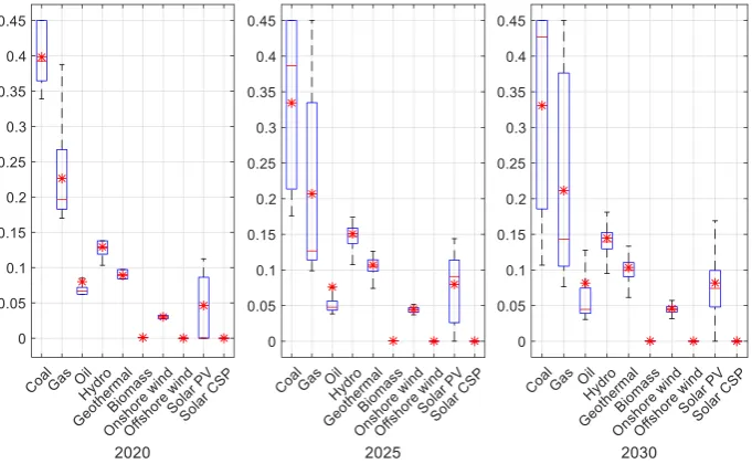
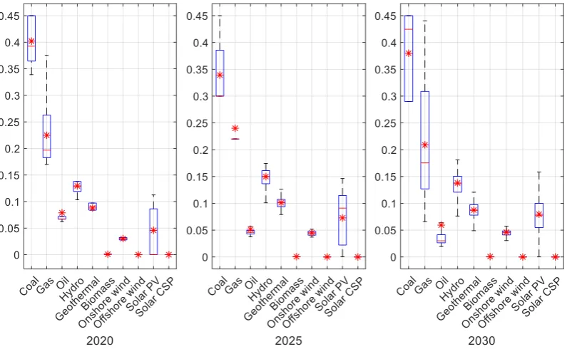
InFig. 4, the optimised stochastic power generation mix across the whole simulation period is illustrated. Outliers have been removed from the box plot representation, while the weighted mean proportions of the different technologies, xτ in the power generation mix are

denoted by a red asterisk. The central red line in the whisker charts represents the median, while the bottom and top edges of the blue boxes indicate the 25th and 75th percentiles, respectively. The black whiskers cover the non-outliers that represent the most extreme data points. It should be highlighted that the illustration with the boxplots can demonstrate the range of potential output values; however, the likelihood of occurrence of each realization can be only found through the weighted average output value (asterisk symbol), which indicates the expected value of the results (here the power production proportion of each technology in the mix), taking into account all scenarios and their probabilities. Under the baseline scenario, power generation from coal appears to decrease throughout the planning horizon from 40% to 34%, NG power generation experiences a slight decrease from 21% to 19%, which is covered by the increasing share of hydro, geother-mal, onshore wind and solar PV.

Total mean weighted installed power capacity was calculated 81.6 GW in the 2020 baseline case, increasing to 210 GW in 2030 due to the growing energy demand. Constraints imposing the renewable tech-nologies penetration, as well as lower carbon emission levels appear to slow down the increase in the installed capacity of coal, as opposed to the NG and renewable energy capacity which appear to increase at a rapid pace over the planning horizon (as shown inFig. 5). In fact, coal installed capacity is predicted to increase by 93.5% from 2020 to 2030 time periods, while NG, hydro, geothermal, onshore wind and solar PV are projected to grow by 118.5%, 131.6%, 164.6%, 250% and 319.4%, re-spectively. Furthermore, new total weighted installed capacity was esti-mated 33.8 GW in 2020, 70 GW in 2025 and 92.4 GW in 2030, weighted RES share was 37.6% in year 2030, CO2,eqemissions were 526 million

tons and total discounted cost was calculated $ 531 billion. The model failed tofind an optimum solution for around 5% of the total uncertainty scenarios, meaning that not all constraints could be satis_fied under

Fig. 4.Optimised power generation mix throughout the simulation period under the Baseline Case.

these scenarios. Results illustrated here were, thus, cleansed and their probabilities were readjusted to sum up to one.

6.2. Sensitivity analysis

Above results were derived under the assumption that the MCS sample of fuel prices follows a normal distribution. InFig. 6, stochastic power generation mixes for the 2025 planning period, under the as-sumption of uniform, PERT and Weibull probability distributions, are shown. The equivalent PERT, Weibull and uniform distributions were based onfitting the baseline normal distribution. In general, results ap-peared not to deviate largely in relation to normal distribution, with deviations observed for uniform distribution predicting 12.5% less coal, 30% more NG and 20% more oil share in relation to the baseline case.

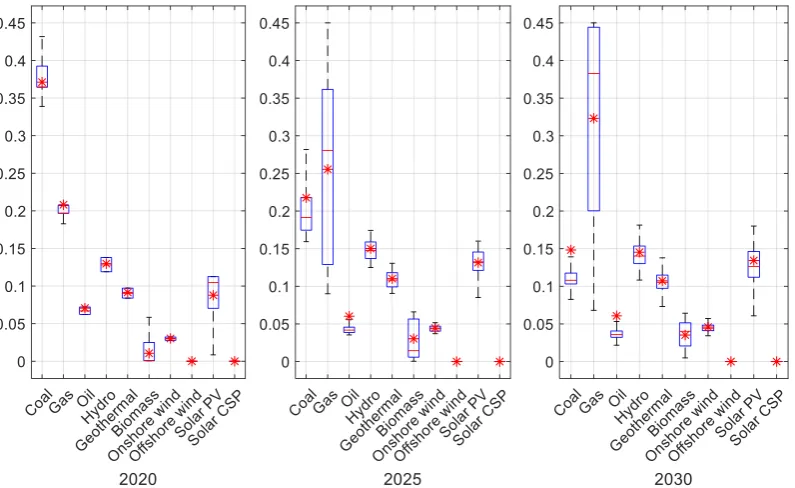
Applying the ST approach to all three uncertain parameters, in-cluding the fuel prices, requires the definition of three discrete nodes corresponding to the fuel prices values (assuming the same number of nodes as in the case of capital costs and energy demand uncertainty) with their assigned probabilities. To test how results would differ in such a case, we ran the model taking the values summarised in Table 5and assigning probabilities similar to the other uncertain

parameters (low: 0.3, medium: 0.5, high: 0.2). The resulting boxplots are illustrated inFig. 7.

ComparingFig. 7withFig. 4, it can be shown that the weighted aver-age results demonstrate significant differences. Furthermore, the length of the box plots resulting from the ST approach is smaller than the one derived from the hybrid uncertainty modelling. This outcome is reason-able as if we apply the ST approach to model uncertainty in the fuel prices by means of three nodes (following the same pattern as the other two uncertain parameters), the number of scenarios would amount to: 33 _{= 9, 3}6 _{= 729 and 3}9 _{= 19,683 for 2020, 2025}

and 2030 time periods, respectively (hence less than the number of sce-narios under the hybrid uncertainty modelling: 1350, 12,150, 109,350 for 2020, 2025 and 2030 time periods, respectively).

The benefit of employing the MCS lies in the fact that it allows for a continuous distribution to be assigned on the selected parameter based on collected historical data rather than assigning a degree of belief to possible scenarios.

It has to be noted that one of the key assumptions allowing for the combination of the ST and MCS methods is the averaging of the MCS out-puts (i.e. the new installed capacity of the power plants which are, sub-sequently, used as input in the next time period) by the end of each time period to reduce the dimensionality of the problem and make it compu-tationally feasible. If the averaging did not take place, the number of sce-narios would amount to: 150·33_{= 1350, 150}2_·36_{= 1.8·10}6 _and

1503_·39_{= 2.5·10}9_{for 2020, 2025 and 2030 time periods, respectively,}

creating nodes originating from the tails of the probability distributions, leading to scenarios that may be infeasible to solve (i.e. due to too high fuel prices) and requiring very high computational effort to deal with. This would also increase the number of outliers and potentially the length of the boxplots to incorporate the outputs with lower probabili-ties. Nevertheless, the weighted mean proportion (xτ) of power

genera-tion accounting for the probabilities of all scenarios is not expected to deviate substantially. Taking the above into consideration, it can, there-fore, be deduced that the boxplots (for example the ones shown inFig. 4) directly incorporate the fuel price uncertainty occurring on the Fig. 5.Weighted average installed capacity under the baseline case.

Fig. 6.Optimal power generation mix under the 3 different probability distributions for 2025.

Table 5

Values of the discrete nodes assumed for the application of the 3-stage ST.

Fuel price ($/MWh)

Low price scenario

Medium price scenario

High price scenario

Coal 31 36 41

Gas 62 72 82

current time period being examined (by means of the n random values of the MCS), but they indirectly incorporate the fuel price uncertainty of the previous time periods through deriving the most expected output values of these periods resulting from the averaging of the new power plant installed capacities.

6.3. Modelling of planning options (POs)

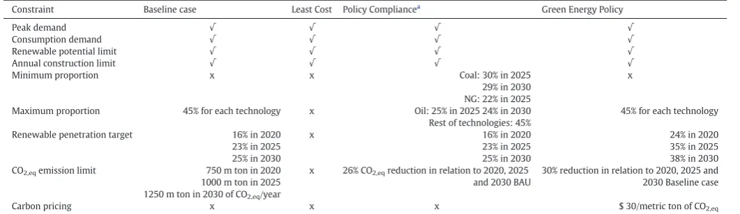
The proposed model was, then, applied to determine the optimal power generation mix for three Planning Options (POs): Least cost, Policy Compliance and Green Energy Policy option. Different sets of constraints were imposed for each option and are summarised in Table 6.

The Least Cost PO focuses only on minimizing the cost of the power generation system, while no carbon emissions limit, renewable contribu-tion and fuel diversity targets are in place. The Policy Compliance opcontribu-tion imposes the renewable energy penetration targets, CO2,eqemission

limits and required coal and natural gas quotas prescribed by the Indonesian's National Energy Policy (NEP). The Green Energy option enforces stricter renewable energy penetration targets and CO2,eq

emission limits. It should be noted that the power generation mix is based on the total power generation of the installed technologies.

6.3.1. Least Cost option

The Least cost option seeks to_find the optimum power generation mix under no renewable energy penetration targets, CO2,eqemissions

targets, or fuel diversity goals; rather, this PO intents to determine the least expensive power generation mix which satisfies the peak and consumption demand, and takes into account the renewable energy potential and annual construction limit of the region. Hence, in the mathematical model, in the inequality (17),REtargettis set to

zero throughout the whole planning horizon, the minimum and maximum proportions of technologies expressed in inequalities (18) and (19) are set to 0% and 100%, respectively, while the carbon emis-sions level targetCtargettin (20) has been set to a very high number so

as not to favour inclusion of greener energy technologies in the opti-mum mix.

The power generation mix of the Least Cost option is dominated by coal power, since there is no imposed carbon emission restriction or re-newable penetration target. Even though the rere-newable penetration in Fig. 7.Optimal power generation mix when developing a three-stage ST.

Table 6

Set of constraints for each PO.

Constraint Baseline case Least Cost Policy Compliancea

Green Energy Policy

Peak demand √ √ √ √

Consumption demand √ √ √ √

Renewable potential limit √ √ √ √

Annual construction limit √ √ √ √

Minimum proportion x x Coal: 30% in 2025

29% in 2030 NG: 22% in 2025

x

Maximum proportion 45% for each technology x Oil: 25% in 2025 24% in 2030

Rest of technologies: 45%

45% for each technology

Renewable penetration target 16% in 2020

23% in 2025 25% in 2030

x 16% in 2020

23% in 2025 25% in 2030

24% in 2020 35% in 2025 38% in 2030

CO2,eqemission limit 750 m ton in 2020

1000 m ton in 2025 1250 m ton in 2030 of CO2,eq/year

x 26% CO2,eqreduction in relation to 2020, 2025 and 2030 BAU

30% reduction in relation to 2020, 2025 and 2030 Baseline case

Carbon pricing x x x $ 30/metric ton of CO2,eq

a

this option is not as high and varied as in other options, it can still fulfil the 25% renewable penetration target for 2030, due to the high contri-bution of the relatively low cost hydropower, as well as the contricontri-bution of geothermal, onshore wind and solar PV power plants. According to the results, overall power generation in 2030 will rely heavily on the three most cost efficient technologies: coal (40%), natural gas (18%), hydropower (14%) and geothermal (10%). The rest of the power gener-ation originates from oil (7%), onshore wind (5%), and solar PV (6%). Cost efficiency accounts both for the total cost of the technology inte-grating the capital,fixed operational, variable operational and fuel

cost, as well as for the total lifetime duration and the capacity factor of each technology. As can be seen fromFig. 8, to satisfy the increasing energy demand at the least cost, the (weighted average) share of coal of the total power production is projected to remain more or less stable until 2030 comprising the dominant energy source of the power gener-ation mix (42% and 40% in 2020 and 2030, respectively) throughout the planning horizon. Natural gas is predicted to undergo a decrease of 14% in its share between 2020 and 2030, while the diesel consumption is projected to experience a 12% decrease between the same timeframe; their reducing contribution is slowly superseded by hydropower Fig. 8.Optimised power generation mix throughout the simulation period under the Least Cost option.

(12% increase from 2020 to 2030), and with small additions in onshore wind and solar PV mainly due to the decreasing trajectories of their future capital costs.

6.3.2. Policy Compliance option

This option encompasses the stochastic power generation mix opti-mization, based on the Indonesian government's policy targets for the power generation sector, as detailed inTable 6. The set of constraints (18)–(19) (Section 4) for this option imposes a minimum natural gas utilization ofMincap2, 2=22% (in 2025) to promote the domestic use of

natural gas. Coal share is also set a minimum limit ofMincap1, 2=30%

by 2025, which in 2030 is reduced to 29%. Furthermore, oil share is set to reach a maximum percentage ofMaxcap3, 2=25% by 2025, which

should decrease to 24% by 2030. A maximum 45% share is imposed to the rest of the technologies to ensure the diversity of the energy mix. As far as the environmental constraints are concerned, theREtargett

throughout the whole planning horizon are adjusted in the model (through inequality (17)) to fulfil the Government's targets and the same applies with the CO2,eqemission limit. As carbon tax has not

been implemented in Indonesia yet,Ctaxt=0 $/ton under the Policy Compliance option.

Fig. 9 shows that the power generation system will be domi-nated by coal, hydro and natural gas-fired power plants, while other re-newable energy technologies such as solar PV and onshore wind are expected to increase their share in the final mix. Coal power growth is limited up to a certain level that satisfies the CO2,eqreduction

and RES penetration targets, reaching a weighted average power generation share of 38% by 2030. The installation of natural gas-fired power plant capacity is driven by the minimum proportion limit im-posed by the policy as well as by the low carbon emissions of the technology.

Furthermore, according to the model output, hydro, geothermal, on-shore wind and solar PV will be employed tofill the gap in 2030 to sat-isfy the increasing power demand. In fact, as the capital cost for onshore wind and solar PV is expected to decrease over the planning horizon, the weighted average new installed capacities until 2030 of onshore wind and solar PV power plants are estimated to reach 14GW and 62.7GW, according to the model.

6.3.3. Green Energy Policy option

The Green Energy Policy option aims to investigate the effect of enforcing progressively stricter targets for the RE penetration (increasing the RES penetration targets by approximately 50%) and mitigation of environmental impact on the power generation mix, throughout the planning period. To this end, a hypothetical carbon pricing was also introduced as a policy for reducing emissions and drive invest-ments into cleaner power generation technologies. Since, no carbon pricing policy is currently in effect in Indonesia, this study assumes an average price ofCtaxt=$30/metric ton of CO2,eq(across all time periods), which is comparable to other studies in literature (Kim et al., 2012;Tran and Smith, 2018;Heck et al., 2016). No constraints on the minimum proportions of power generation technologies in the mix were taken.

As shown inFig. 10, the 2020 power generation mix is again most likely to be dominated by coal due to the existing high installed ca-pacity of the technology, while the gas-fired power generation tech-nology appears to be the second most preferred solution under this set of constraints. However, from 2025 onwards, coal plants are projected to fall sharply (dropping to the level of 14.8% in 2030) with natural gasfired power plants becoming the main electricity producer in the country (25% of power production in 2025 and 32% by 2030). The green energy targets and carbon reduction policies also increase the share of other low carbon technologies. Hydro, geothermal and solar PV power plants are the preferred solutions for covering the largest part of the RES penetration target, while an increasing biomass and onshore wind capacity addition can be observed.

7. Discussion

Fig. 11integrates the values of renewable energy share, discounted total cost, CO2,eqemissions and total new installed capacity of

renew-able energy technologies of the power generation mix under the dif-ferent POs considered. As such, it can be observed that the Least Cost option offers the lowest total discounted cost at the expense of higher CO2,eqemissions, as compared to the other options examined.

Indica-tively, during the planning period 2030, total weighted discounted