City, University of London Institutional Repository
Citation
:
Hazi, A., Martin, P. and Parker, A. (2019). Indecomposable tilting modules for the
blob algebra. City, University of London.
This is the preprint version of the paper.
This version of the publication may differ from the final published
version.
Permanent repository link:
http://openaccess.city.ac.uk/id/eprint/23029/
Link to published version
:
Copyright and reuse:
City Research Online aims to make research
outputs of City, University of London available to a wider audience.
Copyright and Moral Rights remain with the author(s) and/or copyright
holders. URLs from City Research Online may be freely distributed and
linked to.
City Research Online:
http://openaccess.city.ac.uk/
[email protected]
arXiv:1809.10612v2 [math.RT] 10 Sep 2019
INDECOMPOSABLE TILTING MODULES FOR THE BLOB ALGEBRA
A. HAZI, P. P. MARTIN, AND A. E. PARKER
Abstract. The blob algebra is a finite-dimensional quotient of the Hecke algebra of type B
which is almost always quasi-hereditary. We construct the indecomposable tilting modules for the blob algebra over a field of characteristic 0 in the doubly critical case. Every indecomposable tilting module of maximal highest weight is either a projective module or an extension of a simple module by a projective module. Moreover, every indecomposable tilting module is a submodule of an indecomposable tilting module of maximal highest weight. We conclude that the graded Weyl multiplicities of the indecomposable tilting modules in this case are given by inverse Kazhdan–Lusztig polynomials of type ˜A1.
Key words and phrases: blob algebra, tilting modules, KLR algebra, Soergel bimodules.
Introduction
The blob algebra is an extension of the ordinary Temperley–Lieb algebra introduced by the second author and Saleur in [14]. It can be thought of as the Temperley–Lieb algebra of typeB, as it is a quotient of the typeB Hecke algebra in much the same way as the ordinary Temperley–Lieb algebra is a quotient of the Hecke algebra of typeA. Originally motivated by the need to control lattice boundary conditions in lattice models in statistical mechanics, the blob algebra and its generalizations remain an active topic of research in both physics (e.g. [9, 8, 7]) and representation theory (e.g. [18, 19, 1]).
Like the ordinary Temperley–Lieb algebra, the representation theory of the blob algebra is controlled by the values of its parameters. Generically the blob algebra is semisimple, with certain integral representations ∆(λ) calledWeyl modules giving a complete set of simple modules. Yet for some critical parameter values, the blob algebra is only quasi-hereditary, and the Weyl modules are no longer simple. In this paper we focus on the doubly critical case, when the representation theory is the most interesting (e.g. with blocks of arbitrary size, no known quiver-and-relations presentation, etc.). In this case, the block structure is controlled by a linkage principle in terms of an affine Weyl groupW of type ˜A1.
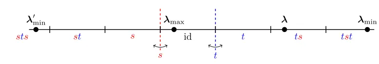
Recall that a tilting module for a quasi-hereditary algebra is a representation with a filtration by Weyl modules as well as a filtration by dual Weyl modules. For each weight λ, there is an indecomposable tilting module T(λ) of highest weightλ, and all indecomposable tilting modules are of this form. Our main result in this paper is a construction of T(λ) for the doubly critical blob algebra Bκ
n over a field of characteristic 0. The construction closely depends on the quasi-hereditary partial orderEon weights, defined in§1.3. TheW-orbit ofλhas one maximal weight
λmax and at most two minimal weights with respect to E. We write L(λ) for the simple head of ∆(λ), P(λ) for the projective indecomposable cover of L(λ), and OEλ(M) for the maximal
submodule of a moduleM whose composition factors lie in{L(µ) :µEλ}. Using this notation, our construction is as follows (see also Theorems 5.3 and 5.4).
Theorem. Suppose λ is a weight for Bκ
n. Let λmin be a minimal weight in the W-orbit of λ. Then T(λ) = OEλ(T(λmax)). The maximal highest weight tilting module T(λmax)is constructed from P(λmin)as follows.
(i) If λmin is the only minimal weight in theW-orbit ofλ, thenT(λmax) =P(λmin).
(ii) If there is another minimal weight λ′min in the W-orbit of λ, then T(λmax) is the unique extension of the form
0→P(λmin)→T(λmax)→∆(λ′min)→0.
2010Mathematics Subject Classification. 20C08.
Figure 1. The (classical) weightsλmax,λmin, andλ′min, with alcoves labelled by wλ.
Forx, y∈W, write
hx,y(v) =
(
vℓ(x)−ℓ(y) ify≤x,
0 otherwise,
which is the inverse Kazhdan–Lusztig polynomial of type ˜A1. Using the decomposition numbers forBκ
n (first calculated in [16]), our construction implies the following Weyl multiplicities for the regular indecomposable tilting modules (see also Corollary 5.5). Here for each regular weight λ, letwλ∈W such thatwλ(λmax) =λ.
Theorem. Let λ,µbe regular weights forBκ n. Then
(T(µ) : ∆(λ)) =hwλ,wµ(1).
See Figure 1 for an example depicting the weight and alcove labels used in these theorems. Our proofs depends in a crucial way not only on the decomposition numbers and structure of the Weyl modules from [16], but also on thegraded representation theory of the blob algebra. The existence of a non-trivial ‘hidden’ grading on the blob algebra is a consequence of the Brundan– Kleshchev isomorphism [2] between cyclotomic Hecke algebras and KLR algebras, which are graded. (This explains why previous work such as [15, 20] on full tilting modules did not get very close to determining the indecomposable tilting modules.) As a bonus we obtain the graded Weyl multiplicities of the graded indecomposable tilting modules with no extra work. Our result is perhaps the first example of how the hidden grading on the blob algebra can be used to solve problems which a priori are not graded at all.
We also make extensive use of KLR diagrammatics for the KLR presentation of the blob al-gebra, as described in [12]. The classical diagrammatic calculus for the blob algebra in terms of ‘Temperley–Lieb diagrams with blobs’ gives a cellular basis which is integral and multiplicative. However, it is difficult in general to describe the simple modules in terms of this basis. By con-trast, KLR algebras have a complicated diagram calculus reflecting the KLR presentation, in which certain fixed parameter values are ‘built-in’ and cannot be changed. On the other hand, KLR di-agrams give more information about the structure of projective modules, in particular whether certain composition factors (or extensions between composition factors) are present. Fortunately for us, we will only need a simplified (but still complicated) version of the KLR diagram calculus. Much of this machinery applies, at least in principle, to the generalised blob algebras (cf. e.g. [1], [17], [12]). For example, the levellgeneralised blob algebras are controlled by an affine Weyl group
Wl of type ˜Al−1, and there is a corresponding KLR presentation. For λa regular weight for the level l generalised blob algebra and λmax maximal in the Wl-orbit ofλ, let wλ ∈ Wl to be the unique element in the affine Weyl group such thatwλ(λmax) =λ. Forx, y ∈Wl, writehx,y for the inverse Kazhdan–Lusztig polynomial of type ˜Al−1.The following conjecture is the natural extension of our Weyl multiplicities result.
Conjecture. Letλ,µbe weights for the levellgeneralised blob algebra over a field of characteristic 0. Then
(T(µ) : ∆(λ)) =hwλ,wµ(1).
The layout of the paper is as follows. In§1 we define the doubly critical blob algebraBκ n using the KLR presentation and describe the corresponding weight combinatorics. In§2 we summarise the quasi-hereditary representation theory ofBκ
n. In§3 we exploit the KLR presentation to obtain bases for the indecomposable projective modules and their composition factors. In §4 we get to work with KLR diagrammatic calculations which give the main result in the case of singular weights. Finally in §5 we use the singular version to prove the main result for all weights.
Acknowledgements
We thank EPSRC for financial support under grant EP/L001152/1.
1. Preliminaries: the blob algebra Bκ
n
Suppose e >1 is an integer and let I =Z/eZ. An adjacency-free bicharge is an ordered pair κ= (κ1, κ2)∈I2such thatκ1=6 κ2, κ2±1 (this implicitly requirese≥4). Fori∈I define
hi|κi=
(
1 ifi=κ1or i=κ2, 0 otherwise.
For anyn∈N, the symmetric groupSn acts on the set of tuplesIn by permutation. We writesr
for the simple transposition (r r+1) in the symmetric groupSn.
Definition 1.1. Let k be a field, n, e ∈ N, and κbe an adjacency-free bicharge. The (doubly
critical)blob algebra Bκ
n overkis theZ-gradedk-algebra generated by
ψr for 1≤r≤n−1,
(1)
yr for 1≤r≤n,
(2)
e(i) fori∈In,
(3)
subject to relations
e(i)e(j) =δi,je(i) for alli,j∈In (4)
X
i∈In
e(i) = 1 (5)
yre(i) =e(i)yr (6)
ψre(i) =e(sri)ψr (7)
yrys=ysyr (8)
ψrys=ysψr whens6=r, r+ 1
(9)
ψrψs=ψsψr when|r−s|>1
(10)
ψryr+1e(i) = (yrψr−δir,ir+1)e(i)
(11)
yr+1ψre(i) = (ψryr−δir,ir+1)e(i)
(12)
ψ2re(i) =
e(i) ifir+16=ir, ir±1
0 ifir+1=ir
(yr+1−yr)e(i) if ir+1=ir+ 1 (yr−yr+1)e(i) if ir+1=ir−1 (13)
ψrψr+1ψre(i) =
(ψr+1ψrψr+1−1)e(i) ifir+2=ir=ir+1−1 (ψr+1ψrψr+1+ 1)e(i) ifir+2=ir=ir+1+ 1
ψr+1ψrψr+1e(i) otherwise (14)
yhi1|κi
1 e(i) = 0 (15)
e(i) = 0 wheni2=i1+ 1
and a grading defined by
dege(i) = 0, degyre(i) = 2, degψre(i) =
1 ifir+1=ir±1,
−2 ifir+1=ir, 0 otherwise.
In the presentation in Definition 1.1, eache(i) is a (non-central) idempotent, eachψris analogous to the simple transpositionsrin the symmetric groupSn, and eachyris akin to the nilpotent part of the corresponding Jucys–Murphy element in the symmetric group algebrakSn.
There is also a presentation of this algebra in terms of KLR diagrams [12, § 3.2]. A KLR diagram withnstrings consists ofnpaths of the formp: [0,1]→R×[0,1] satisfying the following
properties:
• for each path pwe havep(0) = (x,0) andpr(1) = (x′,1) for somex, x′∈R;
• all intersections are transversal;
• there are no triple intersections;
• each path may be decorated with a finite number of dots at non-intersection points.
Each pathpis also labelled with a residuei∈I.
We consider KLR diagrams up to isotopy; in other words, we are allowed to move these paths continuously as long as the properties above still hold and no intersections are added or removed. Thebottom (resp.top) of a KLR diagram is the sequence of residues labelling the paths, ordered by the relationp≺p′ ifp(0)< p′(0) (resp.p≺p′ ifp(1)< p′(1)). The product of two diagramsD
and D′ is defined to be their vertical concatenation (with D on top ofD′) whenever the bottom
of D equals the top of D′. Otherwise the product is defined to be 0. The diagrammatic blob algebra Bκ
n is then the set of all k-linear combinations of KLR diagrams with nstrings, with a diagrammatic product defined byk-linear extension, subject to the following relations:
= −δij
= −δij
=
if|i−j|>1,
− ifj=i+ 1,
− ifj=i−1,
0 ifi=j.
in all regions of a KLR diagram, whereα= 1 wheni=k=j−1, α=−1 when i=k=j+ 1, andα= 0 otherwise, as well as the relations
= 0, ifi1=κj for somej,
= 0, ifi16=κj for allj,
= 0, ifi2=i1+ 1.
Ifw=sr1sr2· · ·srkis a reduced expression inSn, we writeψw=ψr1ψr2· · ·ψrkfor the product of
the correspondingψ-generators. Diagrammaticallyψw (or more precisely,ψwe(i) for somei∈In) looks like the wiring diagram for w. We also write ( ) for the unique anti-involution which fixes each of the generatorsψr,yr, ande(i).
1.1. Locality. We call a relation in the generators ofBκ
n local if the relation still holds when the indices of the generators are shifted by some amount. All the relations in Definition 1.1 above are local except for (15) and (16). The relation (15) is also the only one in which κ appears. Incidentally it is immediately clear that all other relations do not depend on precise values of sequences i ∈ In indexing the idempotents, but only on relative differences i
r+1−ir for some integer 1≤r≤n. In fact for any i∈I, ifκ′ = (κ
1+i, κ2+i) then we haveBκn ∼=Bκ
′
n, and this isomorphism maps e(i)7→e(i+ (i, . . . , i)). Thus Bκ
n only depends on the difference κ1−κ2 ∈I up to isomorphism.
When simplifying KLR diagrams we adopt the convention of circling regions in some colour wherever we apply a local relation only involving ψ-generators. These circles are only a helpful annotation and should not be considered an intrinsic part of the diagram. Similarly whenever we apply relations (11) or (12) in the distinct residue case, we will draw a coloured arrow parallel to the string to indicate how the y-generator ‘slides’ along the string. The most important non-local relation which we will use takes the following form.
Lemma 1.2. Let i∈In and1≤r≤n−1 be an integer such that |i
r−ir+1|= 1 bute(sri) = 0 in Bκ
n. Then yr+1e(i) =yre(i). Proof. Apply (13) to obtain
yr+1e(i) =yre(i)±ψr2e(i) =yre(i)±ψre(sri)ψr=yre(i).
When applying Lemma 1.2 to a KLR diagram, we will draw a dashed coloured line transverse to the strings to indicate which idempotente(i) we are using, and a coloured arrow to show where they-generator ‘jumps’ to a different string.
Theorem 1.3 ([19, Corollary 3.6]). Suppose e >1 is an integer which is not a multiple of the characteristic of k. Let m be an integer with 1 < m < e−1. Set κ = (0, m), an
adjacency-free bicharge. Then Bκ
n has a presentation as an ungraded algebra over k, with generators Ur for 0≤r≤n−1 subject to the following relations:
Ur2=−[2]Ur if1≤r≤n−1,
UrUsUr=Ur if|r−s|= 1 and1≤r, s≤n−1,
UrUs=UsUr if|r−s|>1 and0≤r, s≤n−1,
U1U0U1= [m+ 1]U1,
U02=−[m]U0,
where [k] = [k]q =q−k+1+q−k+3+· · ·+qk−1,q is ane′th primitive root of unity in k, and
e′=
(
2e ifeis even,
e otherwise.
Remark 1.4.
(1) The statement of [19, Corollary 3.6] uses the bichargeκ= (k,−k) (wherek∈I such that 2k≡m (modn)) and a ‘negative variant’ form of (16). To transform this into Theorem 1.3 it is necessary to shift the residues by−k(as mentioned in§1.1) and apply the isomorphism
R(0,n −m)−→Rn(0,m)
ψr7−→ −ψr
yr7−→ −yr
e(i)7−→e(−i)
of cyclotomic KLR algebras with bicharges (0,−m) and (0, m).
(2) Theorem 1.3 is the most general version of what is commonly stated in the literature, but it can probably be extended to other cases as well. For example, when eequals the characteristic ofk,Bκ
nbehaves like the classical blob algebra overkwithq= 1. In addition, adjacency-freeness ofκand the condition that 1< m < e−1 can potentially be relaxed, at the cost of modifying relation (16) (this is similar to what happens for the Temperley–Lieb algebra [19, Remark 3.7]).
1.3. Weights and multipartitions. In general the representation theory of KLR algebras is gov-erned by the combinatorics of multipartitions, while that of the blob algebra is naturally govgov-erned by the geometry of a suitable weight lattice [17]. To understand the blob algebra in KLR terms it is enough to focus on one-column bipartitions.
Aone-column bipartition ofnis an ordered pairλ= (1λ1,1λ2) withλ
1, λ2∈Z≥0andλ1+λ2=
n. We write Λ(n) for the set of all one-column bipartitions ofn. The mapping
Λ(n)−→ {−n,−n+ 2, . . . , n−2, n} λ7−→λ1−λ2
is a bijection between one-column bipartitions and the classical weight set for the blob algebra. For this reason we will usually call one-column bipartitionsweights when working in a representation-theoretic context. For two weights λ,µ ∈ Λ(n) we write λ ⊳ µ (and say µ dominates λ) if
|λ1−λ2|>|µ1−µ2| (following [16]).
TheYoung diagram forλ∈Λ(n) is defined to be the set
[λ] ={(r,1) : 1≤r≤λ1} ∪ {(r,2) : 1≤r≤λ2}
Elements of this set are usually calledboxes, because the traditional way to depict Young diagrams is as a collection of boxes, e.g.
[(14,15)] =
,
A tableau of shapeλis a bijection [λ]→ {1,2, . . . , n}, which is usually depicted by writing each assignment inside the corresponding box, e.g.
9 4 3 1
,
2 5 6 7 8
A tableau is calledstandardif the entries in the boxes increase going down each column. A standard tableau t corresponds in a natural way to a sequence t|k ∈ Λ(k) of Young diagrams obtained by
adding exactly one box at each stage. Such sequences are in bijection with paths of lengthnon the global lattice of weightsZ, where a path is just a functionp:{0,1,2, . . . , n} →Zwithp(0) = 0 and p(k+ 1)−p(k) =±1 for all integers 0≤k≤n−1. Adding a box in the first column corresponds to a rightward (+1) step and vice versa.
We write tλ for the standard tableau of shape λ obtained by labelling the boxes of [λ] with increasing entries ordered from left to right and from top to bottom like a book, e.g.
t(14,15)=
7 5 3 1
,
2 4 6 8 9
The (κ-)residue of a box with coordinates (r, m) is defined to be κm+ 1−r∈I. Theresidue sequence it of a tableautis the sequence of residues of the boxes (t−1(1),t−1(2), . . . ,t−1(n)). We
write iλinstead ofitλ for the residue sequence of the dominant tableautλ.
2. Cellularity of Bκ
n
Supposetis a standard tableau of shapeλ. Letdt∈Snbe the permutation such thatdttλ=t.
Theorem 2.1 ([19, Theorem 6.8]). Fix a reduced expressiondt for each dt over allλ∈Λ(n)and
t∈Std(λ). The elements
ψst=ψdse(iλ)ψd−1
t ∈B κ n
over all λ ∈ Λ(n) and all s,t ∈ Std(λ) form a graded cellular basis for Bκ
n with respect to the partial order Eon weights and the anti-involution ψ7→ψ. In other words
For the precise definition of a graded cellular basis see [10, Definition 2.1]. An important corollary, especially in conjunction with Lemma 1.2, is the following.
Corollary 2.2. Let i∈In. If there is no standard tableau t with (κ-)residue i, then e(i) = 0 in
Bκ n.
Remark 2.3.
(1) The degree of ψst does not depend on the choices of ds or dt, and has a combinatorial definition based onsandt(see Theorem 2.7 below).
(2) The graded cellular structure on Bκ
n is in fact graded quasi-hereditary, which we will use frequently from now on. The idempotent-truncated algebras e(iλ)Bκ
ne(i λ
), studied extensively in [18, 12] are also graded cellular but are not quasi-hereditary.
2.1. Graded cellular and quasi-hereditary algebras. We fix some notation for graded mod-ules. If M = L
jMj is a graded vector space, we define the grade shift Mhki for k ∈ Z by
Mhkij = Mj−k. For M, N graded Bκ
n-modules, we call a degree-preserving homomorphism
M → N homogeneous of degree 0. When we write HomBκ
n(M, N) we always mean the space
of ungraded homomorphisms. By convention any homomorphism we write with a grade shifted object is homogeneous of degree 0, but homomorphisms without grade shifts may be ungraded.
We recall some facts about graded cellular and quasi-hereditary algebras [10]. Let λ∈ Λ(n), and writeBκ,⊲λ
n for the subspace spanned by all basis elements indexed by standard tableaux for weights µ⊲λ. Cellularity essentially means that for any standard tableauxs,t∈Std(λ), we can
write the action ofBκ
n on the basis vectorψs,t modulo the subspaceBnκ,⊲λas
aψst=
X
v∈Std(λ)
where the scalarsrsv(a) don’t depend ont. We can use these scalars to define a module ∆(λ) with basisψsindexed by Std(λ), namely
aψs=
X
v∈Std(λ)
rsv(a)ψv
We call such modules cell modules or Weyl modules. Graded cellularity means that there is a degree function on tableaux (see Theorem 2.7) which makes the basis{ψs}a homogeneous basis. For any fixed standard tableaux a,b∈Std(λ), we can define a contravariant bilinear form on ∆(λ) by
ψasψtb=hψs, ψtiψab (modBnκ,⊲λ)
In fact this bilinear form does not depend on a or b. For a general cellular algebra the quotient
∆(λ)/radh−,−iis either a simple module, which we callL(λ),or 0. The non-zero quotients give a complete list of non-isomorphic simple modules up to grade shift. In our case, none of the quotients are zero because Bκ
n is quasi-hereditary. We write P(λ) for the graded projective cover ofL(λ). ForM a gradedBκ
n, we define the graded composition factor multiplicities [M :L(λ)]v=
X
k
[M :L(λ)hki]vk ∈Z
≥0[v±1],
where [M : L(λ)hki] denotes the number of composition factors in a graded composition series isomorphic toL(λ)hki. Similarly ifM has a graded Weyl filtration, we define
(M : ∆(λ))v=
X
k
(M : ∆(λ)hki)vk ∈Z
≥0[v±1],
where (M : ∆(λ)hki) denotes the number of subquotients in a graded Weyl filtration isomorphic to ∆(λ)hki. For the ungraded counterparts of these multiplicities we use the same notation but without the subscriptv.
As Bκ
n is quasi-hereditary, we also have the notion of a tilting module. A tilting module for
Bκ
n is a module with a filtration by Weyl modules as well as a filtration by dual Weyl modules. For each weight λ, there is an indecomposable tilting moduleT(λ) of highest weight λ, and all indecomposable tilting modules are of this form [21]. In the graded setting this classification only gives a grading onT(λ) up to grade shift. We will fix the grading so that (T(λ) : ∆(λ))v= 1.
The anti-involution gives rise to a duality functor on Bκ
n-modules which reverses grade shift. The unshifted simple moduleL(λ) is self-dual, so the dual Weyl module∇(λ) has socle isomorphic to L(λ). Similarly the unshifted injective envelopeI(λ) is isomorphic to the dual of P(λ). By highest weight considerationsT(λ) is self-dual. Forh∈Z≥0[v±1], we writeh=h(v−1).
2.2. Tower of recollement. For fixed m, eand varying n, the family of classical blob algebras (with presentation as in Theorem 1.3) has the structure of a tower of recollement [4, Example 1.2(ii)]. A tower of recollement consists of a collection of algebras and idempotents in these algebras which satisfy certain axioms, giving rise to several functors between module categories which pass representation-theoretic information between the algebras. Constructing the functors and verifying the axioms are both more easily accomplished in the classical presentation of the blob algebra. For this reason we will assume for the moment that Theorem 1.3 holds so that the tower of recollement structure transfers to {Bκ
n}n∈N. For the basic definitions and some examples
see [4, Section 1], and [15, Section 3] for applications. For eachn∈Nwe have a pair of adjoint functors
ind :Bκ
n−mod−→Bκn+1−mod, res :Bn+1κ −mod−→Bnκ−mod
called induction and restriction respectively. As a right adjoint functor, restriction is left exact, and similarly induction is right exact. However, restriction also happens to be right exact as well. Forλ∈Λ(n+ 1) writeλ= (1λ1,1λ2). Ifλ
1≥λ2>0 we have a short exact sequence
0 /
while res ∆(1n+1,∅) = ∆(1n,∅). When 0< λ
1≤λ2 there are similar exact sequences with the two outer terms switched. Induction on Weyl modules also produces exact sequences in this way, but without a boundary exception.
We also have another pair of adjoint functors
G:Bκ
n−mod−→Bκn+2−mod, F :Bκn+2−mod−→Bκn−mod
called globalisation andlocalisation respectively. Again localisation is right exact as well as being left exact. For λ= (1λ1,1λ2)∈Λ(n+ 2) we have
F∆(1λ1,1λ2) =
(
∆(1λ1−1,1λ2−1) ifλ
1, λ2≥1,
0 otherwise.
and similarly for ∇(λ) and L(λ) [15, Proposition 3]. Moreover, as long as λ1, λ2 ≥ 1 we also have P(λ), ∇(λ), I(λ), and T(λ) by [5, A1(4)], [5, Proposition A3.11], and [5, Lemma A4.5]. This implies thestability of decomposition numbers and tilting multiplicities across alln. In other words, for all n∈N andλ,µ∈Λ(n) with λ= (1λ1,1λ2) andµ= (1µ1,1µ2), the decomposition
number [∆(µ) :L(λ)] only depends onλ1−λ2 andµ1−µ2 but not onn.
For λ = (1λ1,1λ2) ∈ Λ(n) globalisation behaves similarly for Weyl modules and projective
modules, with
G∆(1λ1,1λ2) = ∆(1λ1+1,1λ2+1), GP(1λ1,1λ2) =P(1λ1+1,1λ2+1)
butnotfor simple modules, dual Weyl modules, injective modules, or tilting modules. Globalisation is exact on the full subcategory of ∆-filtered modules [15, Proposition 4]. It also acts as a right inverse for localisation, i.e.F◦Gis naturally isomorphic to the identity.
Finally we have the key relationship between induction/restriction and localisation/globalisation, which is the natural isomorphism
ind∼= res◦G.
In the case ofBκ
n, the tower of recollement structure behaves well with the anti-involution so the dual statement
res∼=F◦ind
also holds.
2.3. Linkage principle. There is a linkage principle for the blob algebra, in terms of the following alcove geometry. LetW be the infinite dihedral group acting onZgenerated by reflectionsskabout
the integers (κ1−κ2) +ke for anyk ∈Z. Each alcove consists of the integers (κ1−κ2) +ke <
j < (κ1−κ2) + (k+ 1)e lying between two adjacent reflection points. Weights lying inside an alcove are called regular, while those on a reflection point are singular. The fundamental alcove is the unique alcove containing the integer 0. Two integers are called linked if they are in the same
W-orbit. The group W also acts partially on paths inZ. For a path p, if p(k) is the reflection
point (κ1−κ2) +je, then we write
sk jp(r) =
(
p(r) ifr≤k,
sjp(r) ifr > k.
In other words,sk
jpis the path obtained by reflectingpafter thekth point. We say that two paths are linked if one can be obtained by a sequence of reflections of the other.
Write Stdλ(µ) for the set of standard tableaux of shapeµwith residue sequence iλ. It turns out that this set can be described entirely in terms of the alcove geometry above, using the fact that weights and tableaux correspond to points in Zand paths inZrespectively.
Proposition 2.4 ([18, Lemma 4.7]). Let λ,µ∈ Λ(n). Under the tableau-path bijection, the set Stdλ(µ)corresponds to paths which end atµin the same linkage class as tλ.
linkage class of tλ. The other 3 paths in this linkage class are illustrated in black from the point
where they diverge fromtλ.
−6 −2 0 2 6
These paths correspond to the tableaux
, ,
2
5
6
8 7 3
4
9 1
9 8 7 6 5 2
3
4 1
, 1
3
4
5
6
7
8 2
9
1 2
3
4
5
6
7
8
9
Corollary 2.6. If [∆(µ) :L(λ)]6= 0 thenµandλare in the same linkage class.
A consequence of the above result is that if λ,µ∈ Λ(n) are in different linkage classes, then they are also in different blocks. We write prλ for the functor which projects modules and ho-momorphisms onto the block(s) of simple modules parametrised by weights in the linkage class of
µ.
The degrees of tableaux in Stdλ(µ) can also be calculated from their corresponding path. We call a subsequence of e consecutive steps in a path a wall-to-wall step if the steps start from a wall (i.e. a reflection point) and continue in a single direction until they reach another wall. For t ∈ Stdλ(µ) a standard tableau write w(t) for the number of wall-to-wall steps across the
fundamental alcove.
Theorem 2.7 ([18, Theorem 4.9]). Let t ∈ Stdλ(µ). Let δ(t) be 1 if the first step after all
wall-to-wall steps points toward the origin, and 0otherwise. Then degt=w(t) +δ(t).
Finally we describe the decomposition numbers in characteristic 0 in terms of the alcove geom-etry. For any regular weightλ, there exists a unique weightλfundin the fundamental alcove and
wλ∈W such thatwλ(λfund) =λ. Forx, y∈W, definehy,x by
hy,x(v) =
(
vℓ(x)−ℓ(y) ify≤x,
0 otherwise.
This is the Kazhdan–Lusztig polynomial associated toW (in the notation of [22]).
Theorem 2.8([18, Theorem 5.11]). Supposekis a field of characteristic0. Letλ,µbe two regular
weights lying in the same linkage class. Then we have
[∆(µ) :L(λ)]v =hwµ,wλ(v).
to a positive classical weight (i.e. a weight on the right side of the origin in our pictures). Working inductively, fork even (resp. odd) we define λk+1 to be the rightmost (resp. leftmost) weight in the linkage class distinct fromλ0,λ1, . . . ,λk. Similarly, whenλcorresponds to a negative classical weight, for k even (resp. odd) we define λk+1 to be the leftmost (resp. rightmost) weight in the linkage class distinct fromλ0,λ1, . . . ,λk.
Theorem 2.9 ([18, Theorem 5.14]). Supposek is a field of characteristic 0. Let λbe a singular
weight. Then if λk is defined we have
[∆(λk) :L(λ)]v=vk.
Remark 2.10. In general, it is easier to use tableaux when working with permutations of the form dt for some tableau t of shape λ, as one can read off dt directly from the two tableaux t and tλ. By contrast, it is easier to use paths in order to apply Proposition 2.4. We will mostly use tableaux in the arguments below, but the careful reader may use the tableau-path bijection in order to translate our arguments into the language of paths if necessary.
3. Bases for projective indecomposable modules
For the rest of this paper, we will assume that k is a field of characteristic 0. Most of the
previous results are known to hold in some form for the classical blob algebra. To proceed further we must make use of the KLR-style presentation ofBκ
n, and in particular the grading. 3.1. A Temperley–Lieb subalgebra. AsBκ
n is graded, it has a subalgebra of degree 0 elements. This subalgebra was classified in [12,§5.4–5.5]. We summarise their results below.
Definition 3.1. Letλ= (1λ1,1λ2)∈Λ(n). Suppose the weightλ does not lie in the interior of
the fundamental alcove. We definefλ to be the minimal positive integer such that thefλth point of the path corresponding totλ lies on a wall of the fundamental alcove. In other words,
(17) fλ=
(
min({2λ2+ (κ1−κ2) +je:j∈Z} ∩N) ifλ1≥λ2, min({2λ1−(κ1−κ2) +je:j∈Z} ∩N) ifλ1< λ2.
Forj∈Nwritef(j) =fλ+je. For all j∈Nsuch thatf(j)≤n−ewe define thediamond of
λat positionf(j) to be
(18) Uλ
j = (ψf(j))(ψf(j)−1ψf(j)+1)(ψf(j)−2ψf(j)ψf(j)+2)· · ·
· · ·(ψf(j)−e+1ψf(j)−e+3· · ·ψf(j)+e−3ψf(j)+e−1)· · ·
· · ·(ψf(j)−2ψf(j)ψf(j)+2)(ψf(j)−1ψf(j)+1)(ψf(j))e(iλ). The name ‘diamond’ comes from the corresponding KLR diagram for this element, e.g.
for e = 6. The cyclotomic KLR algebra versions of these elements previously appeared in [11, (4.2)], while the effect of similar permutations on paths was seen even earlier, e.g. [13, Figure 4].
Theorem 3.2 ([12, Theorem 5.24]). Let λ ∈ Λ(n). The diamonds of weight λ generate the degree 0 subalgebra of e(iλ)Bκ
ne(i λ
). This subalgebra is isomorphic to a Temperley–Lieb algebra with loop parameter2(−1)e−1, with the diamond at position f
Temperley–Lieb diagrammatic generator at index j. In other words, the diamonds of weight λ
satisfy the relations
Uλ i U
λ j =U
λ j U
λ
i when|i−j|>1,
Uλ
i UjλUiλ=Uiλ when|i−j|= 1, (Uλ
i )
2= 2(−1)e−1Uλ
i for alli,
and this gives a complete presentation of the subalgebra generated by them.
Recall that in quantum characteristic 0 the Temperley–Lieb algebra is semisimple, with a unique 1-dimensional irreducible module. The central idempotent corresponding to this irreducible module is sometimes called theJones–Wenzl projector. We write JWλ for the corresponding idempotent in e(iλ)Bκ
ne(i λ
). In our notation, one of the defining properties of JWλ is that Uλ jJW
λ
= 0 for allj.
Lemma 3.3. Let λ∈Λ(n). Then P(λ)∼=Bκ nJW
λ.
Proof. ClearlyBκ nJW
λis an indecomposable projective module, as JWλis a primitive idempotent for the Temperley–Lieb subalgebra (and thus also fore(iλ)Bκ
ne(i λ
) andBκ
n). SupposeBκnJW λ
=
P(µ). ThenBκ
n maps onto ∆(µ), which induces a surjective homomorphism
e(iλ)BnκJW λ−→
e(iλ)∆(µ)
of e(iλ)Bκ ne(i
λ
)-modules. By the defining property of JWλ, the degree 0 part of the domain is 1-dimensional. On the other hand, the degree 0 part of the codomain is the cellular module of weight µ for the Temperley–Lieb subalgebra. (Here we use the fact that the cellular structure of the Temperley–Lieb subalgebra is compatible with that of e(iλ)Bκ
ne(i λ
), because the latter is positively graded by Theorem 2.7.) This has dimension strictly larger than 1 unlessµ=λ.
3.2. Maximal degree tableaux. The following key combinatorial lemma constructs maximal degree tableaux, which are of fundamental importance in the characteristic 0 representation theory ofBκ
n.
Lemma 3.4. Let λ∈Λ(n)be a weight. For eachµ∈Wλwith λEµ, there is a unique tableau
tµ
λ∈Stdλ(µ)of maximal degree
degtµλ =
(
ℓ(wλ)−ℓ(wµ) ifλ is regular,
k ifλ is singular andµ=λk.
Proof. Let t ∈ Stdλ(µ), and write d for ℓ(wλ)−ℓ(wµ). From Theorem 2.7 recall that degt is
either w(t) or w(t) + 1, where w(t) is the number of wall-to-wall steps inside the fundamental
alcove for the path corresponding to t. By Proposition 2.4 t lies in the linkage class of tλ. The
path corresponding totλcontainsℓ(wλ)−1 wall-to-wall steps, whereas any path with endpoint µ
must have at leastℓ(wµ)−1 wall-to-wall steps outside the fundamental alcove to get there. Thus
w(t) is bounded above byd.
There are four cases, according to the parity ofdand whether λandµlie on the same side of the origin or not. We will focus on one of these cases; the other three are similar. Suppose dis even and thatλandµboth lie on the same side of the origin. First we note that since paths toλ
t∈Stdλ(µ). There exists a tableautµλ∈Stdλ(µ) withw(tµλ) =dmaximal, e.g.
−6 −2 0 2 6
Moreover, this tableau is unique: for any such path, the wall-to-wall steps inside the fundamental alcove must occur as early as possible. If not, the path would have to leave and then return to the fundamental alcove, wasting wall-to-wall steps in the process. Finally, tµ
λhas maximal degree too. From the picture above degtµ
λ=w(t µ
λ), and for all other tableauxtwe have degt≤w(t) + 1≤(w(tµλ)−2) + 1<degtµλ
Remark 3.5. An alternative proof of this result uses [12, Theorem 4.9] to reduce the problem of determining graded dimensions of Weyl modules to a calculation in the Iwahori–Hecke algebra corresponding to W. The result follows from the observation that the ‘Bott–Samelson’ elements (i.e. products of simple Kazhdan–Lusztig generators) in this algebra are just sums of Kazhdan– Lusztig basis elements.
An interesting application of these maximal degree tableaux is the following lemma, which identifies composition factors of Weyl modules in terms of the cellular basis.
Lemma 3.6. Let λ∈Λ(n), and supposeµ∈Wλ withλEµ. Consider the submoduleBκ nψtµ
λ of the Weyl module ∆(µ). Then there is a homomorphism
Bκnψtµ
λ −→L(λ)hdeg tµλi
ψtµ
λ 7−→ψtλ.
Proof. Letd= degtµλ=ℓ(wλ)−ℓ(wµ). From Theorem 2.8 we have
[∆(µ) :L(λ)]v =hwµ,wλ(v) =v d,
so the Weyl module ∆(µ) contains exactly one subquotient isomorphic toL(λ)hdi. Recall that
L(λ) is generated by a vector of residue iλ in degree 0. This means that the unique subquotient of ∆(µ) isomorphic to L(λ)hdi is generated by some vector of residueiλ in degreed. But from Proposition 2.4 and Lemma 3.4 we have
dimve(iλ)∆(µ) =
X
t∈Stdλ(µ)
vdegt
=vd+ l.o.t.
In other words, the subspace of vectors with the correct residue and degree is one-dimensional,
spanned byψtµλ, so the result follows.
Applying Brauer–Humphreys reciprocity, we can also identify the Weyl subquotient isomorphic to ∆(µ) insideP(λ).
Corollary 3.7. Letλ∈Λ(n), and supposeµ∈WλwithλEµ. There is a surjective homomor-phism
Bκ nψtµtµ
λJW
λ−→∆(
µ)hdegtµ
λi
ψtµtµ λJW
λ7−→
where the domain is a submodule ofBκ nJW
λ∼ =P(λ).
4. Singular projective modules
The aim of this section is to determine the socles of the indecomposable projective modules associated to singular weights — Theorem 4.13 and Corollary 4.14. This turns out to be enough to completely determine the structure of these modules. The result will then be used in §5.1 to address the corresponding (harder) non-singular cases.
Our general strategy is to identify possible generators for the socle in Lemma 4.7 and then to rule out all but one of them via direct computation. The computation involves the Jones– Wenzl projector, which is difficult to work with directly because in the standard basis it is a sum with many terms. Luckily nearly all of these terms combine or vanish in the computation when multiplied by certain cellular basis elements.
In this section we will assume thatn≡κ1−κ2 (mode), or in other words that there is a wall at n. Fixη = (1n,∅)∈Λ(n) and letm ∈Nsuch that n=f
η+me(see (17) for a definition of
fη). Recall how the linkage class of η consists of the weights ηj for some non-negative integers
j. The maximal weight in this linkage class is ηm, which is on a wall of the fundamental alcove. Note that fηj =fη+je, because the distance fromηj to the nearest fundamental alcove wall is (m−j)esteps.
4.1. Cellular basis factorization. We begin with a factorization of some of the distinguished cellular basis elements from the previous section.
Proposition 4.1. For all integers0≤j≤k≤mwe have
ψtηktηk
ηj =xjxj+1· · ·xk−1ψfη+jeψfη+(j+1)e· · ·ψfη+(k−1)ee(i
ηj )
for some elements xr∈Bκn (with j≤r < k) which satisfy the following properties: (i) for fixed rthe elementxr does not depend onj or k;
(ii) for r6=s,xrxs=xsxr andxrψfη+se=ψfη+sexr;
(iii) for each rwe have
xrxr=e(iηk),
xrxr=e(sfη+rei
ηj).
Proof. Letd=dtηk
ηj. Recall thatdis the permutation which maps
tηk totηk
ηj.
For 0≤l≤m, write ηl= (1ηl,1,1ηl,2) and setr
l= 2 min(ηl,1, ηl,2). From (17) it is clear that
fηl=fη+le=
(
rl+fη ifl is even,
rl+ (e−fη) ifl is odd.
This means that
rl=
(
le ifl is even,
(l−1)e+ 2fη ifl is odd.
Thus the integers 1 ≤r≤rj lie in the same boxes in the tableauxtηj, t ηk
ηj, and t
ηk so we have
d(r) =r. Similarly whenrk < r≤n,ris in the same box in bothtηk andt ηk
ηj so d(r) =rhere as well.
Forj≤l < k, the boxes intηk
ηj with labelsrl< r≤rl+1 form the skew tableau
ifl is odd,
while the same boxes intηk form the skew tableau
ifl is even,
ifl is odd.
This of course means that d restricted to rl < r ≤ rl+1 is still a permutation dl. In fact dl corresponds to a triangular portion of the lower half of a ‘diamond permutation’:
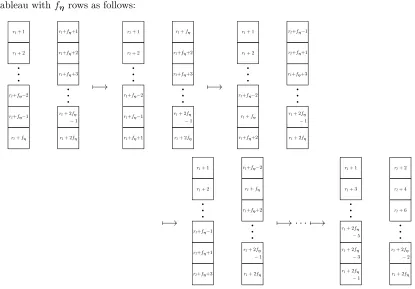
tableau withfη rows as follows:
7−→ 7−→
7−→ 7−→ · · · 7−→
The number of layers in the triangle is eitherfη−1 ore−fηdepending on parity. But 2≤fη ≤e−2, so in both cases the corresponding diagram in the blob algebra factors asxlψfη+lewithxlgenerated
by transpositions of degree 0. Properties (i)–(iii) follow immediately.
Example 4.2. Letn = 21, e = 6 and κ = (0,3). The weightη = (121,∅) is singular because 21≡3−0 (mod 6). Observe thatη1= (13,115) and thatη3= (19,112). Then
ψtη3tη3
η1 = .
We also have
x1x2= .
Some immediate consequences of Proposition 4.1 include the following corollaries.
Corollary 4.3. For all integers0≤j ≤k≤l≤m we haveψtηltηl ηkψt
ηktηk ηj =ψt
ηltηl ηj.
Corollary 4.4. For all integers0≤j ≤k≤mwe have
ψtηk ηjt
ηk ηj =ψ
2 fη+jeψ
2
fη+(j+1)e· · ·ψ 2
fη+(k−1)ee(i
ηj ).
4.2. Vanishing terms. It will be important to know later that certain products vanish in Bκ n. Somewhat surprisingly this can happen even when the total degree is small.
Lemma 4.5. We have
ψtη1tηη1ψtηη1tη1 =ψ
2 fηe(sfηi
Proof. From Proposition 4.1 it is clear that the first product above vanishes if and only if the second product vanishes. We expand the first product by pulling apart the double transposition of degree 2 and rewriting as a difference of dotted strings. In the first term, the left string with its dot can be pulled all the way to the left, because the residues of all the strings that it passes through are distinct. In the second term, the dot on the right string can jump almost all the way to the left, slide down a string, and then make one final jump to the leftmost string. Dots on the left vanish inBκ
n, so we are done. The diagrams below depict this process whenfη = 4.
= −
= −
= −
= 0−0.
Another useful fact is that many cellular basis elements have a diamond as a factor, and thus vanish when multiplied by JWη.
Proposition 4.6. Suppose k < l≤2k. Lett∈Stdη(η
l)with degt= 2k−l. Then ψttηl η ∈U
η jBκn for somej∈N.
Proof. Since degt= 2k−l < k < lit is clear thatt6=tηl
η . This means that the path corresponding to t must diverge from that of tηl
or like
or their mirror images.
Suppose we are in the first case, e.g. withtcorresponding to the black path below:
Letu∈Sn be the permutation which swaps the one-column partitions in the skew tableau above and fixes everything else. As these columns contain two adjacent subsets of e entries each, u
corresponds to a diamond permutation. Writeufor standard the reduced expression forucoming from Definition 3.1. Applying utotyields a new tableaut′ with the same residue (corresponding
to the blue path above). In the path picture, it is clear that the region in grey bounded byt′ and t is entirely contained within the region bounded by tηl (the red path) and t. This means that
dt=udt′ as reduced expressions (see e.g. [12, Algorithm 5.2]). Thus
ψttηl
η =ψuψt′t ηl η =U
η jψt′tηl
η ∈U
η jB
κ n
which proves the result.
Letu′ be the following permutation in blue
which we call a ‘cut diamond’ permutation, corresponding to the first
(
2e−fη ifj is even,
e+fη−1 ifj is odd
layers of the diamond permutation centred atfη+je, and fix u′ to be the corresponding reduced expression foru′. Applying u′ totyields a new tableaut′ (corresponding to the blue path above),
whose entries within the skew tableau are given by
firste layers
7−−−−→
remaining layers
7−−−−−−→
where we have written the increments in the omitted boxes with +1 or +2. Working in the path picture, we again note that the region in grey bounded by t′ and t is entirely contained with
the region bounded by tηl (the red path) and t. As before this means that d
t = (u′)−1dt′ as
reduced expressions. From Proposition 4.1 we also know thatxjψfη+jee(i
η) is a factor of ψ tηltηl
η .
Moreover, from the proof of this proposition, there is a reduced expressionu′′(which comes from the
complement of the ‘cut diamond’ in the KLR diagram above) for whichxjψfη+jee(i
η
and u= (u′)−1u′′. In fact, the construction oft′ ensures thatd
t′ commutes with u′′, because the
support of u′′ (i.e. the elements not fixed by u′′) is fixed by d
t′. Combining everything together,
we get
ψttηl
η =ψ(u′)−1ψt′tηlψtηlt ηl
η ∈ψ(u′)−1ψdt′ψu′′e(i
η )Bκ
n =ψ(u′)−1ψu′′e(i
η )ψdt′B
κ n⊆U
η jBκn.
The next result identifies possible candidates for generators of the socle ofP(η).
Lemma 4.7. IfsocP(η)contains a copy ofL(η)h2kifor somek≥0, then it must be the subspace
kJWηψtηk η t
ηk η JW
η
Proof. L(η) is 1-dimensional, so it restricts to the unique 1-dimensional irreducible representation of the Temperley–Lieb subalgebra. This means JWη acts on it as the identity, and thus any submodule isomorphic toL(η)h2kilies in the degree 2kpart of JWηBκ
nJW η
. From Corollary 3.7, all cellular basis elements ψ6=ψtηk
η t ηk
η with top and bottom residuesi
η
and degree 2k which do not vanish in P(η) = Bκ
ne(i η
)JWη have the form ψ =ψ ttηl
η for some integer k < l ≤ 2k with
degt = 2k−l. By Proposition 4.6 such basis elements factor as ψ = Uη
jx for some j ∈ N and
x∈Bκ
n. Since JW η
Ujη = 0 the result follows.
4.3. Diamond simplification. By Lemma 4.7, determining the socle of P(η) will necessitate calculations involving JWη. The next few lemmas give some methods for reducing the workload by eliminating diamonds.
Lemma 4.8. For all kwe have
ψfη+(k−1)eU
η
kψfη+(k−1)e=±ψ 2
fη+kee(sfη+(k−1)ei
η ).
Proof. Apply [12, Lemma 5.16] several times across the diamond. The remaining transpositions are all of degree 0 except for the degree 1 transpositions at the top and bottom. The degree 0 transpositions cancel out and the result follows. The diagrams below depict what happens when
e= 6.
=− =
=− =· · ·
· · ·= (−1)e = (−1)e
Lemma 4.9. For all kwe have
UkηUkη−1ψ2fη+ke=±Ukηψf2η+(k −1)e.
Proof. This follows immediately from a variant of Lemma 4.8, which is proved in the same way.
= (−1)e
Lemma 4.10. For all1< k < mwe have
Ukη−1ψtηk
η tηηk = 0.
Proof. Use Proposition 4.1 to rewrite ψtηk η t
ηk
η as a product of double transpositions. Expand the
rightmost double transposition as a difference of dotted strings. First we show that these dots can ‘migrate’ leftwards until they lie on top of the next pair of transpositions. In the first term, the dot on the left string can jump until it is on the right string above this double transposition. In the second term, the dot on the right string can slide along the southwest border of the diamond, jump left one string and slide until it is in place on the left string above the double transposition.
= −
= −
northwest until it is in the correct position.
− = −
= −
= −
Note that in both of the figures above we are only drawing a portion of the complete diagram. Finally we end up with a difference of dotted strings for the leftmost double transposition. But we can replace this difference with another double transposition. Applying Lemma 4.5 gives the
result.
4.4. Socle calculation. We pool together our previous results into one grand calculation to iden-tify the socle of P(η). The heart of the argument is to show that certain products of JWη with cellular basis elements do not vanish inBκ
n. This is potentially extremely difficult, as the number of summands when JWη is written in the standard monomial basis grows very quickly. Thankfully many of these monomials end up vanishing in the product. Forr≤swriteUη
r,s=UrηU η
r+1· · ·Usη. First, we identify a non-vanishing monomial in the product.
Theorem 4.11. Let r≤s. If
ψtη1tη1 η U
η r,sψtηk
η t ηk η JW
η6= 0
then (r, s) = (1, k). In this case, we have
ψtη1tη1 η U
η 1,kψtηk
η t ηk η JW
η =±ψ
tηηk1+1tηηk+1JW η.
Proof. Whenr >1, we have
(19) ψtη1tη1
η U
η r =U
η1 r−1ψtη1tη1
η
by Proposition 4.1. Similarly whenr > k, we have
(20) Uη
rψtηk η t
ηk η =ψt
ηk η t ηk η U η r. When 1< r≤swe have
ψtη1tηη1U
η r,sψtηk
η t ηk η =U
η1
r−1,s−1ψtη1tηη1ψtηηkt ηk η
=Uη1
r−1,s−1ψtη1tη1 η ψ
2 fη+eψ
2
fη+2e· · ·ψ 2
fη+(k−1)e
=Uη1
r−1,s−1ψtη1tη1 η ψt
η1 η t
η1 η ψ
2
fη+2e· · ·ψ 2
fη+(k−1)e
= 0
using (19), Corollary 4.4, and Lemma 4.5. Similarly whenr≤s≤k−1 this expression vanishes by Corollary 4.4 and Lemma 4.10. Finally
Uη r,sψtηk
η tηηkJW
η =Uη r,s−1ψtηk
η tηηkU
η sJW
η= 0
ifs > kby (20) and the defining property of JWη. Putting this all together, if
ψtη1tηη1U
η r,sψtηk
η t ηk η JW
η6 = 0
Using Corollary 4.4 and Lemma 4.9, we observe that
ψtη1tη1 η U
η 1,kψtηk
η t ηk η JW
η
=ψtη1tη1 η U
η 1,k−2U
η k−1U
η kψ
2
fη+(k−1)eψ 2
fη+(k−2)e· · ·ψ 2 fη+eJW
η
=±ψtη1tη1 η U
η 1,k−2U
η k−1U
η kU
η k−1ψ
2 fη+keψ
2
fη+(k−2)eψ 2
fη+(k−3)e· · ·ψ 2 fη+eJW
η
=±ψtη1tη1 η U
η 1,k−1ψ
2
fη+(k−2)eψ 2
fη+(k−3)e· · ·ψ 2 fη+eψ
2
fη+keJW
η.
Apply this several times to obtain
ψtη1tη1 η U
η 1,kψtηk
η t ηk η JW
η =±ψ tη1tη1
η U
η 1ψf2ηψ
2 fη+2eψ
2
fη+3e· · ·ψ 2
fη+keJW
η.
Then by Lemma 4.8 and Corollaries 4.3 and 4.4 this is equal to
±ψtη1tη1 η ψ
2 fη+eψ
2 fη+2eψ
2
fη+3e· · ·ψ 2
fη+keJW
η
=±ψ2fη+eψ2fη+2eψ 2
fη+3e· · ·ψ 2
fη+keψtη1tη1 η JW
η
=±ψtηk+1 η1 tη1
ψtη1tηηk+1
1
ψtη1tη1 η JW
η
=±ψtηk+1 η1 t
ηk+1
η JW
η .
Next, we show that other monomials wind up in an ideal ofBκ n.
Theorem 4.12. Let U be a monomial in the generators of the Temperley–Lieb subalgebra. If
U 6=U1,kη then
ψtη1tη1 η U ψtηηkt
ηk η JW
η ∈
Bκ,⊲ηk+1
n .
Proof. Every monomial in the generators of the Temperley–Lieb subalgebra can be written in the form Uη
r1,s1U
η r2,s2· · ·U
η
rp,sp for some strictly decreasing sequences r1 > r2 > · · · > rp and
s1> s2>· · ·> sp of some lengthp≥0 with rj ≤sj for allj. SupposeU 6=U1,kis a monomial of this form such that
ψtη1tη1 η U ψt
ηk η t ηk η JW η6 = 0.
First of all we must havep≥1 by Lemma 4.5. Since rj > rp ≥1 and sj > sp ≥rp ≥1 for all 1≤j < p, we can apply (19) to the expression above:
ψtη1tη1 η U
η r1,s1U
η
r2,s2· · ·U
η
rp−1,sp−1U
η
rp,spψtηηkt ηk η JW
η =
=Uη1
r1−1,s1−1U
η1
r2−1,s2−1· · ·U
η1
rp−1−1,sp−1−1ψtη1tηη1U
η
rp,spψtηηkt ηk η JW
η .
Theorem 4.11 then implies thatrp= 1 andsp=k. Assuming U 6=U1,k, we must havep >1. Now suppose sp−1> k+ 1. Applying Theorem 4.11 again as well as (19) and (20), we observe that
Uη1
sp−1−1ψtη1tη1 η U
η 1,kψtηk
η t ηk η JW
η =±Uη1
sp−1−1ψtηη1k+1tηηk+1JW η
=±ψtηk+1 η1 t
ηk+1
η U
η sp−1JW
η
= 0.
This is a factor of the previous expression, so it follows that sp−1 =k+ 1. Thus it is enough to show that
ψtη1tη1 η U
η k+1U
η 1,kψtηk
η t ηk η JW
η
=±Uη1
k ψtηk+1 η1 t
ηk+1
η JW
η ∈
Bκ,⊲ηk+1
n . Using Corollaries 4.3 and 4.4 this is equal to
±Uη1
k ψ 2 fη+keψ
2
fη+(k−1)e· · ·ψfη+eψtηtη1 η JW
η
In the proof of Proposition 4.1 we showed that Uη1
k =zk+1xk+1ψfη+(k+1)e for some zk+1 ∈B κ n. Thus we obtain
±Uη1
k ψ 2 fη+keψ
2
fη+(k−1)e· · ·ψfη+eψtηtη1 η JW
η ∈
Bnκψtηk+2tηk+2
η JW
η ≤
Bκ,⊲ηk+1
n .
Finally we are in a position to calculate the socle.
Proof. Since P(η) has a Weyl filtration and the socle of every Weyl module is L(η), it is clear that socP(η) is the direct sum of copies ofL(η). The graded decomposition numbers for singular weights (from Theorem 2.9) indicate that the socle can contain at most one copy ofL(η)h2kifor each integer 0≤k≤mand no copies ofL(η) in odd degree. The submoduleL(η)≤∆(ηm)≤P(η) gives one copy of L(η) of degree 2min the socle. By Lemma 4.7, if socP(η) does contain a copy ofL(η)h2kifor somek < m, then it must be spanned by
JWηψtηk η t
ηk η JW
η .
We will prove that this vector does not generate a copy ofL(η) in the socle by showing that
ψtη1tη1 η JW
ηψ tηk
η t ηk η JW
η6= 0.
Write JWη as a sum of monomials. It is known that the coefficient ofU1,kη in JWη is non-zero (see e.g. [6, Proposition 3.10]), so we may write
JWη =cU1,kη + X monomialsU6=U1η,k
cUU
wherec, cU ∈k andc6= 0. Then using Theorems 4.11 and 4.12 we obtain
ψtη1tη1 η JW
ηψ tηk
η t ηk η JW
η=ψ tη1tη1
η cU η 1,k+ X
monomialsU6=U1η,k
cUU
ψtηk
η t ηk η JW
η
∈ψtηk+1 η1 t
ηk+1
η JW
η
+Bκ,⊲ηk+1
n .
Asψtηk+1 η1 t
ηk+1
η JW
η
/
∈Bκ,⊲ηk+1
n we are done.
Applying the globalisation functor, we see that G∆(η) = ∆(1n+1,1) and GP(η) =P(1n+1,1). Using adjunction we see that
HomBκ
n+2(G∆(η), GP(η)) ∼
= HomBκ
n(∆(η), F GP(η)) = HomBnκ(L(η), P(η))
soP(1n+1,1) also has a simple socle. Repeated globalisation in this manner allows us to drop our assumption on n and extend our result to all singular weights. For a singular weightλ∈ Λ(n), write λmin,λmax ∈ Λ(n) for the unique minimal and maximal weights respectively in the same linkage class.
Corollary 4.14. Letn be arbitrary, and letλ∈Λ(n)be a singular weight. Then we have
socP(λ) =L(λmin)h2 degtλλmax+ degt λ λmini.
5. Main results
5.1. Regular projective modules. We introduce some useful weight terminology. Letλ∈Λ(n). If the linkage class of λ has a uniqueλ′ ∈Λ(n) which is incomparable toλ then we say that λ
is paired. Otherwise we callλ unpaired. For example, every singular weight is unpaired because singular linkage classes are totally ordered. On the other hand the poset structure of a regular linkage class means that the only regular unpaired weights are either maximal (i.e. are contained in the fundamental alcove) or possibly minimal.
Lemma 5.1. Let λ = (1λ1,1λ2) ∈Λ(n) be a regular weight. Then λ is unpaired if and only if
ℓ(wλ) = 0or |λ1−λ2|<2ℓ(wλ)e−n.
Proof. Suppose thatλ is not contained in the fundamental alcove and thatλ1> λ2. Let wλ′ be the unique element ofW such that ℓ(w′
λ) =ℓ(wλ) butwλ′ 6=wλ. Sinceℓ(w′λw
−1
λ ) = 2ℓ(wλ), the unique incomparableclassical weight in the global linkage class of (λ1−λ2) is (λ1−λ2)−2ℓ(wλ)e, which does not correspond to a weight in Λ(n) if it is less than −n. The case where λ1 < λ2 is
Generalising our singular terminology, for an arbitrary weight λ∈Λ(n) write λmin∈Λ(n) for some minimal weight in the linkage class of λ and λmax ∈ Λ(n) for the unique maximal weight in the same linkage class. For λ regular it is evident that λmax = λfund. We now can extend Corollary 4.14 to all weights.
Theorem 5.2. Letλ∈Λ(n). We have
socP(λ) =
(
(L(λmin)⊕L(λ′min))h2 degt λmax
λ + degt λ
λmini if λmin is paired,
L(λmin)h2 degtλλmax+ degt λ
λmini if λmin is unpaired.
Proof. We prove the ungraded result first. Note that for anyµ⊲λ in the same linkage class, the ungraded socle of ∆(µ) is
(
L(λmin)⊕L(λ′min) ifλmin is paired,
L(λmin) ifλmin is unpaired.
AsP(λ) is filtered by Weyl modules its socle may only contain copies of these simple modules. Writeλ= (1λ1,1λ2) and without loss of generality supposeλ
1> λ2. Ifλlies in the fundamental alcove, thenP(λ) = ∆(λ) and the result follows by [16, Theorem 9.4], so we will assume thatλdoes not lie in the fundamental alcove. Takek∈Nminimal such thatµ= (1λ1,1λ2+k)∈Λ(n+k) lies on
a wall and letλ(1)= (1λ1,1λ2+k−1)∈Λ(n+k−1). There is a minimal weightλ(1)
min∈Λ(n+k−1) in the linkage class ofλ(1) whose classical weight is only 1 away fromµmin. We observe that
prµ(ind ∆(λ (1)
min)) = ∆(µmin), prµ(ind ∆((λ
(1) min)
′)) = ∆((
µmin)1),
and
resP(µ)∼=F(indP(µ)) =F P(1λ1+1,1λ2+k) =P(λ(1))
using the tower of recollement structure onBκ n. Thus dim HomBκ
n+k−1(∆(λ
(1) min), P(λ
(1)
)) = dim HomBκn+k(∆(µmin), P(µ)) = 1,
dim HomBκ
n+k−1(∆((λ
(1)
min)′), P(λ
(1))) = dim Hom Bκ
n+k(∆((µmin)1), P(µ)) = 1
by Corollary 4.14. This establishes the result forλ(1).
If k = 1, then we are done asλ =λ(1). Otherwise let λ(2) = (1λ1,1λ2+k−2)∈ Λ(n+k−2).
Again, there is at least one minimal weightλ(2)minin the linkage class ofλ(2) whose classical weight is 1 away from λ(1)min or (λ(1)min)′, and if this weight is also paired then there is another minimal
weight (λ(2)min)′. It is clear that prλ(1)(ind ∆(λ
(2)
min)) (and prλ(1)(ind ∆((λ
(2)
min)′)) if it exists) is a minimal weight Weyl module. We also have
prλ(2)(resP(λ(1)))= prλ∼ (2)(F(indP(λ(1)))) ∼
=F(prλ(2)(indP(λ(1))))
=F(P(1λ1+1,1λ1+k−1))
=P(λ(2)).
Thus dim HomBκ
n+k−2(∆(λ
(2) min), P(λ
(2)
)) = 1 (and similarly for (λ(2)min)′ if it exists) and the result
holds forλ(2). Continuing in this fashion, we obtain the ungraded result forλ(k)=λ. The correct grade shift is apparent from the graded decomposition numbers ofBκ
n (Theorem 2.8).
5.2. Tilting modules. We are finally in a position to present the main results of this paper.
Theorem 5.3. Letλ∈Λ(n)be a maximal weight.
(i) If λmin is unpaired, then T(λ) =P(λmin)h−degtλλmini.
(ii) If λmin is paired, thenT(λ)is the unique non-split extension
0→P(λmin)h−degtλλmini →T(λ)→∆(λ
′
min)h−degt λ