A decomposition algorithm for robust lot sizing problem with remanufacturing option

A Decomposition Algorithm for Robust Lot

Sizing Problem with Remanufacturing Option

¨

Oyk¨u Naz Attila1(B)(0000-0002-8055-9052), Agostinho

Agra2(0000-0002-4672-6099), Kerem Akartunalı1(0000-0003-0169-3833), and Ashwin Arulselvan1(0000-0001-9772-5523)

1

Department of Management Science, University of Strathclyde, Glasgow, UK {oyku.attila,kerem.akartunali,ashwin.arulselvan@strath.ac.uk}

2

Department of Mathematics and CIDMA, University of Aveiro, Aveiro, Portugal

aagra@ua.pt

Abstract. In this paper, we propose a decomposition procedure for con-structing robust optimal production plans for reverse inventory systems. Our method is motivated by the need of overcoming the excessive com-putational time requirements, as well as the inaccuracies caused by im-precise representations of problem parameters. The method is based on a min-max formulation that avoids the excessive conservatism of the dualization technique employed by Wei et al. (2011). We perform a com-putational study using our decomposition framework on several classes of computer generated test instances and we report our experience. Bi-enstock and ¨Ozbay (2008) computed optimal base stock levels for the traditional lot sizing problem when the production cost is linear and we extend this work here by considering return inventories and setup costs for production. We use the approach of Bertsimas and Sim (2004) to model the uncertainties in the input.

Keywords: robust lot sizing, remanufacturing, decomposition

1

Introduction

are observed in the production of a wide range of products, such as electronic goods and industrial items (see, Thierry et al. 1995, Guide and Van Wassenhove 2009, Agrawal et al. 2015). Our main focus is to consider the additional deci-sions regarding remanufacturing while constructing an optimal production plan for a discrete and finite time horizon, where the exact values for demands and returned items are known to be uncertain.

Despite the wide range of research on lot sizing problems (see, e.g., Akartunalı et al. 2016), very few studies have focused on lot sizing problems with remanufac-turing (LSR). Preliminary research on LSR problems includes the implementa-tion of the Wagner-Whithin algorithm by Richter and Sombrutzki (2000), which was later extended to one with manufacturing and remanufacturing costs by Richter and Weber (2001). An economic LSR formulation (ELSR) with disposal costs was introduced by Golany et al. (2001), where the ELSR problem was shown to be NP-complete. A dynamic programming algorithm was presented by Teunter et al. (2006), which solves the ELSR problem in O(T4_{) time for a} special case of the problem. In more recent work, Helmrich et al. (2014) have introduced alternative formulations for the ELSR problem, and have shown that the problem with joint or separate setups is NP-hard. The work of Akartunalı and Arulselvan (2016) has shown the tractability of a polynomial time special case and have introduced two classes of valid inequalities for the capacitated version of the problem. However, there is a lack of literature on the impact of uncertainty on these formulations, with the exception of Wei et al. (2011). The present study aims to contribute to the growing research on ELSR problems by studying the implications of parameter uncertainties within the framework of robust optimization.

Robust optimization was first introduced by Soyster (1973), where uncertain parameters are defined through uncertainty sets and a robust optimal solution is defined as one that remains optimal for every parameter representation in an un-certainty set. More recent studies relaxed this conservative assumption, with the seminal work of Ben-Tal and Nemirovski (1998, 1999) constructing uncertainty sets as ellipsoids. Later, Bertsimas and Sim (2004) defined the uncertainty sets as budgeted polytopes, where robust parameter representations are constrained by a specified value. Their approach was applied to traditional lot sizing prob-lems by Bertsimas and Thiele (2006) and adapted to the robust ELSR in Wei et al. (2011). Bienstock and ¨Ozbay (2008) propose a decomposition approach for solving a min-max formulation of the special lot sizing problem consisting in the computation of basestock levels. Robust lot sizing problems have also been considered as particular cases of the general problems addressed in Agra et al. (2016), and Atamt¨urk and Zhang (2007). For comprehensive books on robust optimization we refer the reader to Bertsimas and Sim (2004) and Ben-Tal et al. (2009). For concise overviews on robust optimization methods see Bertsimas and Thiele (2011), Gabrel et al. (2014), Gorissen et al. (2015).

expla-nation of this conservativeness, see Bienstock and ¨Ozbay (2008). A common approach to handle min-max robust optimization problems is to use a variant of the Benders’ decomposition, (see Thiele et al. 2010). Frequently, this decom-position results in the iterative inclusion of rows and columns (Agra et al. 2013; Zeng and Zhao 2013). Such approach is also known as theAdversarialapproach (Gorissen et al. 2015). For solving robust inventory problems, the decomposi-tion framework was introduced by Bienstock and ¨Ozbay (2008) and revisited later by Agra et al. (2016), where demand in each time period is assumed to be uncertain. Our approach for the robust ELSR problem is also motivated by these studies, where our objective is to generate optimal production plans when demands and returns are uncertain. We use the approach of Bertsimas and Sim (2004) to model the uncertainty set as budgeted polytopes, where the variation of the demands and returns in relation to their nominal values is constrained by a specified value. A robust model with recourse is considered where the inven-tory levels are allowed to adjust to the realization of the uncertain parameters. Our contribution is two-fold. Firstly, we model an extended version of the lot sizing problem, wherein we consider uncertainty in both the return and demand sets with set up costs for production. Our second contribution lies in reporting our computational experience with several input classes of costs and inventory levels.

The remainder of this paper is organized as follows: In Section 2, we introduce the deterministic and robust formulations for the ELSR problem. We introduce the robust decomposition algorithm in Section 3, and finally we conclude by presenting preliminary performance results in Section 4.

2

Problem Definition

In addition, we assume that all problem parameters are known. The values of demands and returns are inexact, however, the inputs used to construct the relevant uncertainty sets are known. All cost parameters are time-invariant, and serviceables have a greater holding cost than returned items. Similarly, manu-facturing an item is more expensive than remanumanu-facturing a returned item.

Manufacturing, remanufacturing, disposal and backlogging costs of a single item are represented as m, r, f and b, respectively. The unit holding cost of serviceable (returned) goods are shown as hs (hr). Let the demands (returns) for periods t = 1, . . . , T be Dt (Rt). For modelling the set up decision, we introduce a binary variable yt and a sufficiently big Mt for all t. Variable xmt (xr

t) indicates the number of items manufactured (remanufactured) in time t. Let the the number of items disposed at the end of periodt bedt. Finally, ZtD (ZR

t ) models the scaled deviation of demands (returns) from the nominal value in periodt. We might drop the time indext, to denote the corresponding vector. For instance,ΓR _{will denote the vector inT dimensions with thet}th_component beingΓR

t .

2.1 Classical Deterministic Model

The ELSR problem can be written as: min (x,y)∈Pθ

D,R

(x, y) (1)

where

θD,R(x, y) = T X

t=1

(Kyt+mxmt +rx r

t+f dt+Hts+H r

t), (2) and x = (xm_{, x}r_{) and y are vectors specifying a feasible production plan that} belongs to the set

P :={(xmt , x

r

t, yt)∈R 2T + ×Z

T +:I

r 0+

t X

i=1

(Ri−xri −di)≥0, ∀t= 1, ..., T

Mtyt≥xmt +x r

t, ∀t= 1, ..., T} (3)

As reverse flows do not exist for returns, their inventory levels are restricted to be nonnegative and we ensure that the setup costK is incurred for the time periodtwhenyt= 1, whereMt=

PT

i=tDi . VariablesHts(Htr) model the total cost of serviceable (return) inventory held in periodtand is given by

Hts= max{hs[I0s+ t X

i=1

(xmi +xri −Di)],−b[I0s+ t X

i=1

(xmi +xri −Di)]} (4)

H_tr=hr[I₀r+ t X

i=1

2.2 Uncertainty

In practical cases some of the parameters may not be known in advance. Here we assume the demands Dt and the returns Rt are uncertain, and consider a twostage robust model. The number of items manufactured, remanufactured and disposals (and consequently the set-up decisions) are assumed to be first stage or “here-and-now” decisions. Thus, such decisions are taken before the value of the uncertain parameters is revealed. While the serviceable and return inventory levels are second-stage variables since they are allowed to adjust to the value of the parameters.

We apply the robust optimization approach of Bertsimas and Sim (2004) defining uncertainty sets as budgeted polytopes. The uncertainty on demand and return parameters is considered to be independent from each other. Therefore, an independent uncertainty set for demands (UD), and returns (UR) exist. For each time periodt= 1, . . . , T,parametersΓtD,D¯t,Dˆt(ΓtR,R¯t,Rˆt) are the budget of uncertainty for demands (returns), nominal demands (returns) and maximum deviation in demands (returns) respectively. The robust parameterDt takes its value in the interval [ ¯Dt,D¯t+ ˆDt]. Similarly, Rt takes its value in the interval [ ¯Rt,R¯t+ ˆRt]. Hence, our uncertainty sets are defined as:

UD(ΓD) :={D∈RT+: Dt= ¯Dt+ ˆDtzDt , ∀t= 1, ..., T, z D t ∈Z

D t (Γ

D t )} (6)

UR(ΓR) :={R∈_RT

+: Rt= ¯Rt+ ˆRtzRt, ∀t= 1, ..., T, z R t ∈Z

R t (Γ

R t )} (7) The variables zD

t and ztR in (6) and (7) take their values in the interval [0,1] and are used to indicate a given proportion of the maximum deviations

ˆ

Dt and ˆRt. In order to avoid overconservative parameter representations, the parametersΓD

t andΓtRare introduced to constrainzDt andzRt. More specifically, the cumulative values of scaled deviation variables for demands and returns are required to be strictly less than or equal toΓ_tD andΓ_tR, hence we obtain:

Z_tD(Γ_tD) :={z_tD∈[0,1]t: t X

i=1

z_iD≤Γ_tD,∀t= 1, ..., T} (8)

Z_tR(Γ_tR) :={z_tR∈[0,1]t: t X

i=1

zR_i ≤Γ_tR,∀t= 1, ..., T} (9)

As the inventory levels are allowed to adjust to the uncertain parameters, the variablesHs

t andHtr will depend on the demands and returns. So, for eacht= 1, . . . , T andD∈UD,we have H_ts(D) given from (4), and for eacht= 1, . . . , T

andR∈UR,we haveH_tr(R) given from (5).

We can now extend the deterministic ELSR problem to this uncertain case as a robust min-max formulation:

min

(x,y)∈PD∈maxUD(ΓD) R∈UR_(ΓR₎

whereθD,R_{(x, y) is extended as follows:}

θD,R(x, y) = T X

t=1

(Kyt+mxmt +rx r

t+f dt+Hts(D) +H r

t(R)) (11)

3

Decomposition Approach

As the number of variablesHs

t(D) andHtr(R) is not finite, the inner maximiza-tion problem is not finite. However, practical experience based on decomposimaximiza-tion algorithms for related problems (see, for instance, Agra et al. 2013 for the case of the robust vehicle routing problem with time windows, Agra et al. 2016 for a general class of problems including the robut lot-sizing problem, and Bienstock and ¨Ozbay 2008 for the problem of computing robust basestock levels) has shown that only a few of the values of the uncertainty sets UD_(ΓD_{) andU}R_(ΓR_{) are} necessary to solve the problem.

Here we present a decomposition algorithm that iteratively solves a restricted version of the robust min-max problem (10) with respect to a subset of points of

UD_(ΓD_{) and ofU}R_(ΓR_{) which will be denoted by ˜U}D_{and ˜U}R_{,respectively. We} call this restricted version of (10) as “Decision Maker’s” problem (DMP). Given an optimal solution (x∗, y∗)∈ P to the DMP, we solve a certain maximization problem, which seeks a demand D ∈ UD_(ΓD_{) and return R ∈ U}R_(ΓR_{) that} maximises the total inventory and backlogging costs for the production plan (x∗, y∗)∈ P. We refer to this subproblem as the “Adversarial Problem” (AP). The extreme pointD∗, R∗ generated by AP is used to update ˜UD _{and ˜U}R _and the process is repeated. Convergence is guaranteed through the finiteness of the number of extreme points of the uncertainty sets UD(ΓD) and UR(ΓD). The formal description of this idea is given in Algorithm??.

InitializeU B= +∞,LB= 0,U˜D={D¯},U˜D={R¯}

while(U B−LB)/LB≥do 1. Solve DMP

a. (x∗, y∗) be the solution of min(x,y)∈PmaxD,R∈_U˜D×_U˜RθD,R(x, y) b. SetLB= maxD,R∈U˜D×U˜RθD,R(x∗, y∗)

2. Solve AP

a. (D∗, R∗) = arg maxD,R∈UD×URθD,R(x∗, y∗) b. ˜UD_{= ˜U}D_{∪ {D}∗_{}, ˜}

UR_{= ˜U}R_{∪ {R}∗_} c.U B= min{U B, θD∗,R∗(x∗, y∗)}

end

For the sake of completeness, we give the DMP and the AP. In order to model the DMP, notice that the inner maximization problem in (10) defined for the restricted set ˜UD_×U˜R_,max

D,R∈_U˜D_×U˜RθD,R(x,y),can be written as:

T X

t=1

(Kyt+mxmt +rx r

t+f dt) + max D,R∈_U˜D_×U˜R

T X

t=1

(H_ts(D) +H_tr(R))). (12)

Introducing variableπto indicate the maximum value of the total inventory and backlogging costs over all possible realizations of demands and returns, the DMP can be written as follows:

min T X

t=1

(Kyt+mxmt +rx r

t+f dt) +π (13)

s.t.π≥

T X

t=1

(Hts(D) +H r

t(R)) ∀D∈

˜

UD

∀R∈_U˜R (14)

H_ts(D)≥hsI₀s+ t X

i=1

(xm_i +xr_i −Di) ∀t= 1, ..., T

∀D∈_U˜D (15)

H_ts(D)≥ −bI₀s+ t X

i=1

(xm_i +xr_i −Di)) ∀t= 1, ..., T

∀D∈U˜D (16)

H_tr(R) =hrI₀r+ t X

i=1

(Ri−xri −di)

, ∀t= 1, ..., T

∀R∈U˜R (17)

t X

i=1

(Ri−di−xri)≥0

∀t= 1, ..., T

∀R∈U˜R (18)

Mtyt≥xmt +x r

t ∀t= 1, ..., T (19)

Note that variables Hr

t(R) can be eliminated using equations (17). Given a solution for variables xm_i , xr_i, di,the AP is formulated as follows:

maxπ (20)

s.t.π≤

T X

t=1

(Hts+h r

t X

i=1

( ¯Ri+ ˆRiziR−di−xri)) (21)

Hts= max

hsI0s+

t X

i=1

(xmi +x r

i−( ¯Di+ ˆDiziD)

,

−bI0s+ t X

i=1

(xmi +x r

i−( ¯Di+ ˆDizDi )

∀t= 1, ..., T (22)

I0r+

t

X

i=1

( ¯Ri+ ˆRizRi −x r

i−di)≥0 ∀t= 1, ..., T (23)

t X

i=1 zDi ≤Γ

D t ,

t X

i=1 zRi ≤Γ

R

t ∀t= 1, ..., T (24)

0≤ztDj≤1, 0≤z Rj

t ≤1 ∀t= 1, ..., T (25)

In order to linearize (22), we introduce binary variablestindicating whether inventory is kept or demand is backlogged, and rewrite it as:

Hts≤h s

I0s+ t X

i=1

(xmi +x r

i−( ¯Di+ ˆDizDi )

+M1t(1−st) ∀t= 1, ..., T (26)

Hts≤ −b

I0s+

t X

i=1

(xmi +x r

i −( ¯Di+ ˆDiziD)

+M2tst ∀t= 1, ..., T (27)

4

Experiments

The proposed decomposition algorithm was implemented in Java using Eclipse Mars. Our formulations were implemented and solved as MIPs using Java API for CPLEX 12.6 on an Intel Core i5, 3.30GHz CPU, 3.29GHz, 8 GB RAM machine. Additionally, each run has been restricted to a total running time of 10,000 seconds. The terminating condition for instances with a smaller running time is set as= 0.01, where = U B_LB−LB .

4.1 Data Generation

Data sets have been generated for different levels of four parameter types: num-ber of returns, probability of constraint violation caused by ΓD

greater or less than the remanufacturing cost. Throughout this section, the data sets are abbreviated as “ABCD T”, where each letter indicates the levels of the aforementioned parameters in their given order, withT time periods.

For all data sets, nominal demand is generated randomly in the interval [50,100]. Likewise, returns are generated randomly in intervals [15,30], [25,50] and [35,70], for low, medium and high levels, respectively. Maximum demand and return deviations are calculated as ˆDt= 0.1 ¯Dtand ˆRt= 0.1 ¯Rt . In order to determineΓD

t andΓtR, we use the probabilistic bounds given by Bertsimas and Sim (2004). We set the probability of constraint violation as 0.01, 0.05 and 0.10, for low, medium and high levels, respectively. To determine the setup cost, we use the following equations:K= 0.1 ¯Dminhs,K= 2 ¯DmedhsandK= 5 ¯Dmaxhs, where ¯Dmin = 50,D¯med = 75 and ¯Dmax = 100, for low, medium and high levels. Finally, the disposal cost is set as d = 0.5r when it is less than the remanufacturing cost, and asd= 2rotherwise.

In addition, the holding cost of serviceables is generated in the interval [5,10], through which the remaining cost parameters are defined. We set the holding cost for returns as hr _{= 0.1h}s_{, the backlogging cost as b = 4h}s_{, the manufacturing} cost asm= 2hr_{, and the remanufacturing cost asr= 2h}r _.

4.2 Preliminary Results

To observe the performance of our decomposition algorithm, we analyse the total time requirements for obtaining the smallest possibleU B−LBgap. The following performance measures are preliminary results that are obtained from 16 different data sets for T = 10, and 5 different data sets forT = 50. A total of 10 instances were solved for each data set.

0 0.01 0.02 0.03 0.04 0.05 0.06 0.07 0.08

HHLG HHLL HMLG HMLL

G

ap

Dataset

Fig. 1: Total UB - LB gap for T=10 (when gap is greater than 0.01).

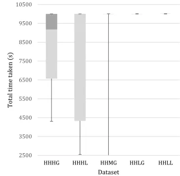
0 1000 2000 3000 4000 5000 6000 7000 8000 9000 10000

HHLG HHLL HMLG HMLL HLLG HHML HLLL

Tota

l time

ta

ke

n

(s

)

Dataset

Fig. 2: Total running time for T=10 (when >0.01 could not be achieved under 10,000 seconds).

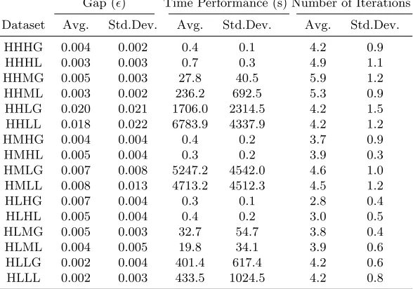
Table 1: Gap, time, iteration performance for T=10.

Gap () Time Performance (s) Number of Iterations

Dataset Avg. Std.Dev. Avg. Std.Dev. Avg. Std.Dev.

HHHG 0.004 0.002 0.4 0.1 4.2 0.9

HHHL 0.003 0.003 0.7 0.3 4.9 1.1

HHMG 0.005 0.003 27.8 40.5 5.9 1.2

HHML 0.003 0.002 236.2 692.5 5.3 0.9

HHLG 0.020 0.021 1706.0 2314.5 4.2 1.5

HHLL 0.018 0.022 6783.9 4337.9 4.2 1.2

HMHG 0.004 0.004 0.4 0.2 3.7 0.9

HMHL 0.005 0.004 0.3 0.2 3.9 0.3

HMLG 0.007 0.008 5247.2 4542.0 4.6 1.0

HMLL 0.008 0.013 4713.2 4512.3 4.5 1.2

HLHG 0.007 0.004 0.3 0.1 2.8 0.4

HLHL 0.005 0.004 0.4 0.2 3.0 0.5

HLMG 0.005 0.003 32.7 54.7 3.8 0.4

HLML 0.004 0.005 19.8 34.1 3.9 0.6

HLLG 0.002 0.004 401.4 617.4 4.2 0.6

As the detailed results in Table 1 indicate, the gaps achieved and number of iterations needed are in general consistent across different data sets, in addition to being in general very small (e.g., the highest maximum gap is still under 0.1, and no more than 8 iterations were necessary for any instance). On the other hand, as it can be also observed from the Figures 1 and 2, the time performance can vary significantly not only among different datasets but also among different instances of most datasets.

When we look into the datasets withT = 50, a greater number of instances naturally run until the maximum time limit is reached as a consequence of the increased number of periods. However, the algorithm is still able to close the gap up to= 0.003 for some instances.

In comparison toT = 10, the total number of iterations reduce as the time limit is reached in earlier iterations. We also observe a greater variety in terms of the total solution time for several data sets (see Figure 4). For groups where the total running time is invariant, the final gap remains larger compared to others, in which case is less than 0.05. The gap, time and iteration performances for

T = 50 are presented in Table 2. Although many instances exhausted the time limit, it is encouraging to see that the maximum gaps still remain very small.

0 0.05 0.1 0.15 0.2 0.25

HHLG HHLL

G

ap

Dataset

Fig. 3: Total UB - LB gap for T=50 (when gap is greater than 0.05).

2500 3500 4500 5500 6500 7500 8500 9500 10500

HHHG HHHL HHMG HHLG HHLL

To

ta

l time

ta

ke

n

(s

)

Dataset

Fig. 4: Total running time for T=50.

5

Conclusions

Table 2: Gap, time, iteration performance for T=50.

Gap () Time Performance (s) Number of Iterations

Data Set Avg. Std.Dev. Avg. Std.Dev. Avg. Std.Dev.

HHHG 0.010 0.006 8203.7 2092.2 3.5 0.7

HHHL 0.012 0.006 7595.5 3305.4 2.8 0.8

HHLG 0.159 0.043 10002.9 1.1 2.1 0.3

HHLL 0.141 0.028 10004.3 1.1 2.0 0.0

HHMG 0.029 0.008 9044.4 3033.3 2.7 0.5

We proposed a simple but effective decomposition procedure for constructing robust optimal production plans, where the approach of Bertsimas and Sim (2004) was used to model the uncertainties in input. Preliminary computational results on various datasets indicate that this procedure can work effectively, in particular to address current issues caused by imprecise representations of problem parameters.

Future work includes further development and improvement of the current computational framework in order to achieve more effective results, in particular of the computational times. It is also important to perform extensive computa-tional testing to allow a thorough statistical analysis of the performance.

References

Agra, A., Santos, M.C., Nace, D., Poss, M.: A dynamic programming approach for a class of robust optimization problems. SIAM Journal on Optimization 26(3), 1799–1823 (2016)

Agra, A., Christiansen, M., Figueiredo, R., Hvattum, L.M., Poss, M., Requejo, C.: The robust vehicle routing problem with time windows. Computers and Operations Research 40(3), 856–866 (2013)

Agrawal, Vishal V., Atalay Atasu, and Koert Van Ittersum: Remanufacturing, third-party competition, and consumers’ perceived value of new products. Management Science (61)1, 60 – 72 (2015)

Akartunalı, K., Fragkos, I., Miller, A., Wu, T.: Local cuts and two-period convex hull closures for big-bucket lot-sizing problems. INFORMS Journal on Computing 28(4), 766–780 (2016)

Akartunalı, K., Arulselvan, A.: Economic lot-sizing problem with remanufacturing op-tion: Complexity and algorithms. In: Machine Learning, Optimization, and Big Data, MOD. pp. 132–143 (2016)

Atamt¨urk, A., Zhang, M.: Two-stage robust network flow and design under demand uncertainty. Operations Research 55(4), 662–673 (2007)

Ben-Tal, A., El Ghaoui, L., Nemirovski, A.: Robust optimization. Princeton Series in Applied Mathematics, Princeton University Press (October 2009)

Ben-Tal, A., Nemirovski, A.: Robust convex optimization. Mathematics of operations research 23(4), 769–805 (1998)

Bertsimas, D., Brown, D.B., Caramanis, C.: Theory and applications of robust opti-mization. SIAM Review 53, 464 – 501 (2011)

Bertsimas, D., Sim, M.: The price of robustness. Operations Research 52(1), 35–53 (2004)

Bertsimas, D., Thiele, A.: A robust optimization approach to inventory theory. Oper-ations Research 54(1), 150–168 (2006)

Bienstock, D., ¨Ozbay, N.: Computing robust basestock levels. Discrete Optimization 5(2), 389–414 (2008)

Gabrel, V., Murat, C., Thiele, A.: Recent advances in robust optimization: An overview. European Journal of Operational Research 235(3), 471–483 (2014)

Golany, B., Yang, J., Yu, G.: Economic lot-sizing with remanufacturing options. IIE transactions 33(11), 995–1003 (2001)

Gorissen, B.L., Yaniko˘glu, I., den Hertog, D.: A practical guide to robust optimization. Omega 53, 124–137 (2015)

Guide Jr, V Daniel R and Van Wassenhove, Luk N.: The evolution of closed-loop supply chain research. Operations Research 57(1), 10 – 18 (2009)

Retel Helmrich, M.J., Jans, R., van den Heuvel, W., Wagelmans, A.P.: Economic lot-sizing with remanufacturing: complexity and efficient formulations. IIE Transac-tions 46(1), 67–86 (2014)

Richter, K., Sombrutzki, M.: Remanufacturing planning for the reverse Wagner/Within models. European Journal of Operational Research 121(2), 304–315 (2000) Richter, K., Weber, J.: The reverse Wagner/Within model with variable manufacturing

and remanufacturing cost. International Journal of Production Economics 71(1), 447–456 (2001)

Soyster, A.L.: Technical note—convex programming with set-inclusive constraints and applications to inexact linear programming. Operations Research 21(5), 1154–1157 (1973)

Teunter, R.H., Bayindir, Z.P., Den Heuvel, W.V.: Dynamic lot sizing with product returns and remanufacturing. International Journal of Production Research 44(20), 4377–4400 (2006)

Thiele, A., Terry, T., Epelman, M.: Robust linear optimization with recourse. Tech. rep. (2010), technical Report. Available in Optimization-Online

Thierry, M., Salomon, M., Van Nunen, J., Van Wassenhove, L.: Strategic issues in prod-uct recovery management. California management review 37(2), 114–135 (1995) Wei, C., Li, Y., Cai, X.: Robust optimal policies of production and inventory with

un-certain returns and demand. International Journal of Production Economics 134(2), 357–367, (2011)