City, University of London Institutional Repository
Citation
: Gerrard, R. J. G. ORCID: 0000-0002-8932-8752, Hiabu, M., Kyriakou, I. ORCID:
0000-0001-9592-596X and Nielsen, J. P. ORCID: 0000-0002-2798-0817 (2018).
Self-selection and risk sharing in a modern world of life-long annuities. British Actuarial Journal,
23, doi: 10.1017/s135732171800020x
This is the published version of the paper.
This version of the publication may differ from the final published
version.
Permanent repository link:
http://openaccess.city.ac.uk/21515/
Link to published version
: http://dx.doi.org/10.1017/s135732171800020x
Copyright and reuse:
City Research Online aims to make research
outputs of City, University of London available to a wider audience.
Copyright and Moral Rights remain with the author(s) and/or copyright
holders. URLs from City Research Online may be freely distributed and
linked to.
City Research Online:
http://openaccess.city.ac.uk/
[email protected]
permits unrestricted re-use, distribution, and reproduction in any medium, provided the original work is properly cited. doi:10.1017/S135732171800020X
Self-selection and risk sharing in a modern world of
life-long annuities
R. Gerrard, M. Hiabu, I. Kyriakou and J. P. Nielsen*
Faculty of Actuarial Science and Insurance, Cass Business School, City, University of London, London EC1Y 8TZ, UK*
[Institute and Faculty of Actuaries, London, 14 May 2018]
Abstract
Communicating a pension product well is as important as optimising thefinancial value. In a recent study, we showed that up to 80% of the value of a pension lump sum could be lost if customer communication failed. In this paper, we extend the simple customer interaction of the earlier con-tribution to the more challenging lifetime annuity case. Using a simple mobile phone device, the pension customer can select the life-long optimal investment strategy within minutes. Thefinancial risk trade-off is presented as a trade-off between the pension paid and the number of years the life-long annuity is guaranteed. The pension payment decreases when investment security increases. The necessary underlying mathematicalfinancial hedging theory is included in the study.
Keywords
Pension; Life-long optimal investment strategy; Customer communication
1. Introduction
It has long been a hen-and-the-egg question in modern pension product development to decide where to start alleviating the many problems with opaque products that most people fail to understand. Many pension savers end up receiving suboptimal pension products that might be optimal for other people. An obvious reason for this is the poor communication. Pension communication has been notoriously difficult due to opaque products and cases with contradicting interests between pension providers and pension receivers. Also,financial advice is expensive and becomes even more so if it is based on opaque products with contradicting interests. An extreme solution to thisfinancial advice question is to give all customers the same one-size-fits-all product. Another extreme is to let the pension saver make all the important investment decisions, even when he is not educated enough to carry out such a difficultfinancial optimisation.
This paper provides a simple intuitive framework that most pension savers would be able to under-stand. Within a few minutes, the pension saver should be able to select the optimal investment strategy
based on individual preferences offinancial risk. Our main point is that, during this task, it is not necessary or relevant to know about the complicated underlyingfinancial mathematical hedging. We suggest solving the financial communication problem of the risk of life-long pension annuities by changing the way that pension products are constructed, so that there is a one-to-onefit between the simple communication and the complicated underlying financial hedging. We believe we offer a genuine solution to the pension crisis challenge articulated by Merton (2014). We are not aware of any other solution enabling the pension saver to design the entire investment guarantee within a few minutes via a simple question that the pension saver can understand. Many alternative pension designs might be possible in future developments with the same set of positive features. Therefore, the reader should not dwell too long on our particular design, but on the fact that pension annuity products can be constructed in a way that pension savers can make informed decisions. Our specific solution incorporates many of the suggested pension principles in Merton (2014), shaped in a format that is simple to implement. Our approach builds on the recent research by Gerrardet al. (2017, 2018) and Donnellyet al. (2018) where similar tools and investment strategies are provided for the simple lump sum case. Gerrardet al. (2017, 2018) provide an example of a risk-averse investor who could lose up to 80% of his savings, calculated in certainty equivalents, if mistaken for a riskier investor. This paper introduces an approach where the pension saver picks his own risk appetite in a simple way that also exactly back-calculates the pension saver’s optimal investment strategy. A major difference from the existing pension offers is that the pension saver picks the pension product directly without translation. The pension saver’s decision has a one-to-one relationship with thefinancial investment strategy. Most existing pension products would let the pension saver decide whether he is, for example, of high, medium or low risk. Thefinancial institution then translates the pension saver’s message into an investment strategy, but the pension saver’s real interests might be lost in such a translation. Our pension design provides the pension saver with the exact investment strategy he asks for. In addition, the pension saver might change his investment strategy: thefinancial question can be posed again at any given time, perhaps on a yearly basis, and the pension saver might then either adhere to the original or update the strategy based on his risk preferences at that time.
The rest of the paper is organised as follows. In section 2, we explain how the communication of the simple lump sum can be generalised to the more complicated life-long annuity case, without com-promising on the simplicity of financial advice, by diving into individual customer Emma’s per-spective. Section 3 highlights the differences from the classical defined contribution (DC) scheme. Section 4 discusses various details of the pension product. Section 5 presents the stochastic model. Section 6 and the Appendices provide all the mathematical details of the pension product.
2. The Pension Product from Customers
’
Perspective
Emma is 35 years old and wants to invest £300,000 received from an inheritance. The investment should cover a real annuity income after her retirement at age 65. The actuaries need to handle the underlying mortality, inflation and investment risk. We require a product that can be presented in a way that allows her to select her optimal strategy in consistency with herfinancial risk preferences. Our solution is communicated to her in the following simple way:
∙
What is your age, when do you want to retire and what is the amount you want to invest? (See also Figure 1.)∙
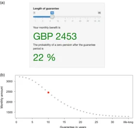
Half of the time your income will continue life long at afixed high level. The other half of the time, it will continue life long at some level between the targeted high level and zero pension.Figure 2a shows the slider Emma can use in order to see the trade-off between the length of guarantee and monthly benefit size. All amounts are in real terms, i.e. in today’s values, subject to future increases with inflation. This facilitates communication as the amount can be compared with today’s purchasing power. Emma can choose between no guarantee, mimicking a classicalfinancial product or a life-long guarantee, mimicking a deferred annuity and hence no exposure to risk. The accom-panying percentage states the chance of ending up with the worst-case scenario of hitting rock bottom zero pension once the guaranteed pension income period is over.
Imagine that Emma chooses a guarantee period of 10 years providing her a monthly real income of £2,453 until at least the age of 75. If investments go well, with a 50% chance, the monthly payments of £2,453 will continue life long. However, there is also the worst-case scenario, with a probability of 22%, that Emma’s pension income will run out when she reaches 75 years of age. In the remaining 28% case, Emma’s life-long annuity will continue with payouts lower than the targeted £2,453. One could imagine that Emma would safeguard herself to minimise the consequences of such an unfortunate investment performance. She could, for example, incorporate the value of her house when reaching 75 years of age, or buy a second product, perhaps a smaller annuity starting when she is 75–but then with a life-long guarantee. The annuity option in this paper could be considered as a building block in a more diverse financial planning of the particular household economy Emma faces. It is beyond the scope of this research to illustrate how a wide array of annuities could provide aflexiblefinancial tool for individual households’financial planning.
[image:4.493.141.342.59.242.2]In Figure 2b, we see the trade-off between length of guarantee and monthly benefit Emma faces. Note that if Emma did not want any guarantee, her most likely pension outcome would exceed £3,000 a year. Alternatively, if Emma wanted absolute lifetime certainty, the guaranteed income would be below £1,500. Emma can gain a lot by taking the risk of not buying a guarantee, and such should be made clear to her via the graph provided. Emma can also discover that by increasing the age at which pay-outs start in Figure 1, a life-long annuity becomes substantially cheaper.
3. Comparison with Traditional-DC Scheme
In this section, we compare the proposed pension product to a typical DC scheme where at retire-ment the lump sum is converted to an annuity.
3.1. Guaranteed Income
In the DC scheme, the pensioner is exposed to (a) risk from thefinancial market, i.e. investment performance in nominal terms, (b) inflation risk, i.e. uncertain development of average living cost and (c) mortality risk, i.e.fluctuations of the annuity price at retirement. These three risks make the
final pension hard to predict. Financial planning is, therefore, a challenge for most pension savers holding traditional DC schemes. Our proposed pension product has a clearly stated minimum monthly income, expressed in real terms, aiding thefinancial planning.
3.2. Performance
[image:5.493.116.393.58.323.2]has more years to diversify the financial investment risk. Second, in our proposed life annuity product, the pension saver receives additional returns equal to the mortality rate. The full trans-parency of our pooled mortality provides our pension saver with a significant extra life-long return. In a DC scheme, the added mortality return is opaque and hidden, hence it is expected to be on the lower side. Both features of our product are expected to result in a significantly higherfinal pension, which is the directfinancial benefit. More importantly, there is also an indirect benefit stemming from the fact that our pension saver is more likely to pick thefinancial risk profile sought, see next.
3.3. Communication
In a classical DC scheme, it is necessary to determine the risk preferences of the pension saver. This is usually done indirectly by means of a procedure that is unrelated with the actual pension, raising the chance of miscommunication and investment in assets that do not fit the actual needs. In our proposed product, the pension saver can directly pick the level of risk sought. He can directly see the trade-off between guarantee and monthly benefit and can pick anything between a no-guarantee product with highest monthly pay-out and a deferred annuity which bears no risk but at the same time gives minimal monthly income. He can also buy more than one product, for example a deferred annuity that starts paying out at age 85 as well as a 20-year guarantee starting at 65. Finally, the choice can be changed at any time by either taking (parts) of the money out or changing the guarantee period.
4. Additional Details
4.1. The Customer Reveals His Risk Appetite
In the above example, Emma revealed her risk appetite in much the same way as proposed for the lump sum case in Gerrardet al. (2017, 2018). By specifying the required guarantee length, Emma directly specifies herfinancial risk appetite. A subsequent simple back-calculation provides us with Emma’s optimal investment strategy. We are in the fortunate situation that the single most important
financial risk question Emma faces is one that she understands, is directly linked to her pension, and she can give an immediate answer to: she wants 10 years of guarantee. Perhaps, this is due to childrenfinishing education by then, and her willingness to sell her house when she is 75 renting a smaller apartment instead. Selling the house would only be necessary if investment income turned out to be too disadvantageous. This is rather unlikely and Emma may maintain her current lifestyle without having to withdraw further from her assets including her house. From a regulatory per-spective, the pension provider selling the annuity has a full record, for future control purposes, of the
financial communication: Emma answered the simple question posed to her with a 10-year period of guarantee ending at the age of 75. The one-to-onefit between communication and pension product drastically reduces the burden of recording thefinancial advice.
4.2. Annuity Principle
from that of a standard life annuity. The main difference is that longevity risk is not transferred to an insurer, but is shared, instead, among the members of the pension fund. The result is an annuity that is transparent in its costs and is actuarially fair.
Whenever an individual in the pension fund dies, his wealth is distributed to the survivors in an actuarially fair way, i.e. at every instant the expected gain (gain when someone else dies less loss of wealth if own death occurs) is zero. Given that the pool is large enough (e.g. 1,000, refer to Donnelly et al., 2013, 2014 for how surprisingly small these annuity pools need to be), the mortality gains are given by
λiðtÞXiðtÞdt;
whereXiis the wealth of individualiandλi(t) the individual’s force of mortality. The relative annuity
gains with magnitudeλi(t) coincide with the growth rate of a fairly priced life-long standard annuity,
hence longevity risk is automatically hedged. If Emma reaches the optimal investment scenario, which happens most of the times, the payouts will continue life long.
4.3. The Overall Principle of Hedging and the Importance of Technical
simplicity
The most important feature of our new class of pension products is the straightforward commu-nication. Another obvious advantage is its simple technical implementation that will help minimising technical errors from actuarial and financial offices. The simplicity will ensure that actuaries and
financial experts are on top of things so that a one-to-onefit is achieved between what actuaries and
financial experts tell other departments and the board of directors and what these interested agents actually get. The hedging strategy can be expressed in terms of a simple probability that actuaries immediately understand. The optimal investment strategy before introducing risk sharing is given by investing the amount
300;000ert+
Ðt
0λiðsÞds
|fflfflfflfflfflfflfflfflfflfflfflfflfflfflfflffl{zfflfflfflfflfflfflfflfflfflfflfflfflfflfflfflffl}
value of 300;000 att
P 0≤ |fflfflfflfflfflfflfflfflfflfflfflfflfflfflfflfflfflfflfflfflfflfflfflfflfflfflfflfflfflffl{zfflfflfflfflfflfflfflfflfflfflfflfflfflfflfflfflfflfflfflfflfflfflfflfflfflfflfflfflfflffl}XiðTiÞ+Pið0Þ300;000ðμrÞTi
terminal wealth of unconstrained strategy corrected by drift
≤GUiðTiÞ jX
iðtÞ
0 B B B @
1 C C C A
in the risky fund, whereμis the average mean return on the risky asset,rthe average inflation per year,tthe time passed since commencement,Tithe time from commencement until the end of the
guarantee period,λithe force of mortality of individuali,Xi the wealth of individualifollowing an
optimal unconstrained strategy,Pið0Þthe initial price of the hedge, andGUiðTiÞthe actuarially fair
price atTifor a life-long annuity; refer to section 6 for further details.
4.4. How Risk is Pooled
individuals want less risk than the safest option. This can be, for example, the case when 100% in the inflation fund still bears too much risk. The individuals can then take advantage of being part of a group. More specifically, the individuals’lack of risk appetite can be circumvented by transferring risk to the rest of the group with a risk appetite (see section 4.4). Finally, in extremely rare cases the entire group loses its aggregate risk appetite, rendering the inflow of investments with risk appetite necessary. This implies the need for an intermediary whose role is described in section 4.4.
4.4.1. Individual
Once the individual has specified the length of his guarantee period, an optimal financial hedge is back-calculated. Thefinancial hedge is based on a risk-free inflation fund and a risky fund. It implies at every point in time a certain risk appetite and an optimal level of inflation hedge. When con-sidering a risky inflation fund, those levels can be recovered by adjusting the proportions of the investments. This result is obtained by lowering the level of investment in the risky fund until the risk appetite from thefinancial hedge is achieved. This implies a slight increase of the investment in the risky inflation fund compared to the original investment in the risk-free fund.
4.4.2. Group
In rare cases, the risk appetite of the individual is so small that risk has to be transferred from the individual to the group. The group, then, chooses, as a solidarity of being part of the group, to borrow money at the risk-free inflation rate and include it in its investments. This allows our pension system to work almost frictionless.
4.4.3. Intermediary
In extremely rare cases with insufficient risk appetite in the group to cover the risk in the inflation fund, an intermediary provides capital with risk appetite. Note that the only promise the inter-mediary makes is to provide risk capital close to the market value. Therefore, it does not cost much to participate. Even so, the intermediary is allowed to charge some administration cost for being the “market maker” to ensure that risk appetite is available at all times and, therefore, ensure the underlying guarantee.
5. The Stochastic Model Underlying the Financial Hedge
In this section, we present thefinancial model used for thefinancial hedging. We choose the simplest possible such model for the sake of transparency, noting that this research output is not aiming for optimal financial modelling. While in this paper we are concerned with connecting investment strategies with annuities and achieving a one-to-one communication to the customer, let us for a second assume that we change the underlyingfinancial model. Thefinancial hedge is about the target income and the length of the guarantee. Changing thefinancial model is expected to only slightly affect the size of the forecasted target income for given guarantees, however the decision of the pension saver remains more or less of the same nature; this approach seems robust under underlying
financial model variations. Therefore, we pick the simplest most transparent model comprising a risk-free inflation fundS0≡1–note that we operate in real terms–and a risky fundS1described via
dS1ðtÞ=μS1ðtÞdt+σS1ðtÞdWðtÞ; (1)
whereμ,σ>0,S1(0)=1 andWis a standard Brownian motion.
risky inflation fund is expected to be constructed in a way that over the long run at least a return of inflation is obtained plus an additional return corresponding to the risk taken in the risky inflation fund. In section 6.5, we will see that a risk transfer can be made from the real investment universe of a risky inflation fund and a more risky fund to the artificial investment universe of a risk-free inflation fund and a risky fund. The transfer simply looks at the risk that thefinancial hedging strategy suggests and downplays the risky fund a little bit while upgrading the risky inflation fund a little bit. This is done until the pension customer has the same risk-return profile, as suggested by the very simple transparentfinancial model (1) consisting of an infeasible risk-free inflation fund and a risky asset.
In the example of section 2, we assume
μ=0:0337;σ=0:1538;
corresponding to 1-year mean returns and standard deviations of 3.43% and 16% for the risky asset (see equations (10) and (11)). The 3.43% return and 16% volatility of the risky asset are from Guillénet al. (2006), based on the empirical results in the book“Triumph of the optimist”(Dimson et al., 2002). In order to price a pension product, the pension provider requires an estimate of the mortality rate,λ(t), of the customer. In Figure 1, this is done by asking for customer’s age. In practice, one may consider more covariates aiming to achieve a better estimate, however such is beyond the scope of this paper. For illustration purposes, we choose for simplicity the mortality rates from the National Life Tables, England, for females in the period 2013–2015 Office for National Statistics (2017). By using this data, we implicitly assume no future period effect on the mortality rates. Again, adopting a more realistic model is possible, but not the focus of this paper. Other information the pension provider receives is the amount of money that the customer wants to invest and the time when payouts should start.
To derive a customer-tailored pension product, it is important to communicate correctly the risk appetite of the customer. Following Gerrardet al. (2017, 2018), it is possible to describe the risk appetite with only one parameter that the customer understands. This is in contrast to an abstract risk aversion parameter of a utility function which is hard to communicate. In Gerrardet al. (2017, 2018), it is shown that, by specifying a minimum amount the pensioner wants to have guaranteed, an optimal investment strategy can be back-calculated, yielding a practically optimal performance specific to the customer’s risk appetite. In section 6.3, we extend this result to the annuity case in which the customer now chooses how long he wants payouts guaranteed. From equation (8), one can then calculate the corresponding size of monthly payouts, so that there is a 50% chance that these continue life long after the guarantee period.
Note that the money paid in should be invested as long as possible. In particular, investments should not stop at retirement, as such would lead to significant losses in expected performance. In our implementation, we choose the investment to last to the end of the guarantee period. A longer investment horizon is not directly possible as it is a priori not known how long the money on the pension account will last. The customer himself is not concerned with these details and only sees Figure 2, visualising the trade-off between guarantee length and monthly benefit size. Once the decision is made, the pension provider is left with an investment strategy due to be implemented.
loss occurs with own death, the full wealth being redistributed. In Proposition 1, we show that in a large pension pool, payouts from it have little volatility and the extra return from entering the annuity scheme is very close to the mortality rate,λ(t).
The theoretical optimal investment strategy is derived in a Black–Scholes world, hence needs to be adjusted to account for model (1). The main idea is that the strategy is adjusted in a way that the calculated optimal risk exposure from the Black–Scholes world is preserved. This is straightforward to do as long as all individuals in the pension fund have enough risk appetite for the adjustment to be feasible, i.e. equation (13) is fulfilled for everyone. If equation (13) is violated for an individual, the risk-sharing principle kicks in: those with sufficient risk appetite in the pension fund offer those who lack risk appetite a risk-free inflation return; refer to section 6.5.1 for more details. The result is that via this risk-sharing principle, everyone maintains the same risk as derived from the Black– Scholes world.
6. The Full Investment Model Including Mortality Risk
In this section, we incorporate mortality in ourfinancial model. While almost any approach to mortality risk can be combined with our new pension design, we have particular preference for the modern risk-sharing approach of Bräutigamet al. (2017) as there are no hidden costs in it to the customers that cover each other’s risk almost without any long-term cost. But again, what follows aims to just illustrate that it is possible to provide an easily communicated pension design including mortality risk. Just as our pension design itself may have several variations with similar positive properties, the underlying mortality approach used for the annuity may also take different shapes without compromising on our overall ideas of a simple pension product that is easy to communicate and where the entire investment strategy can be back-calculated from a short conversation with the pension saver. As pointed out in section 5, we will start with two assets: a risk-free inflation bondS0 and a risky assetS1. Thefinancial hedging principle is based on this simple model; mortality risk will be incorporated in section 6.2. The real investment universe the pension customer faces has a risky inflation fund rather than a risk-free inflation bond. Therefore, there is some risk transfer adjustment to be done, so that the pension saver can maintain the risk–return relationship that the financial hedging suggests. This is carried out in section 6.5.
6.1. Two Asset Case: Inflation Fund and Risky Fund
Let usfirst restate our simple transparentfinancial model used forfinancial hedging. There are two assets: a risk-free inflation bond,S0, and a risky assetS1, described by
dS0ðtÞ=rS0ðtÞdt; dS1ðtÞ=μS1ðtÞdt+σS1ðtÞdWðtÞ; t≥0 (2)
whereμ,σ,r>0 and S0(0)=S1(0)=1. The only source of randomness is the standard Brownian motion, W, defined on a complete probability space ðΩ;F;PÞ. The information available to the investor is represented by the filtration Ft=σfWðsÞ;s20;tg _ N ðPÞ, where N ðPÞ denotes the
collection of allP-null sets so that thefiltration obeys theusual conditions. We denote byXi(t) the
amount of wealth invested by individualiin the fund at timet, of whichπi(t) is invested in the risky
the fund defined by dCiðtÞover the time interval (t,t+ dt). Hence,
dXiðtÞ=r Xð iðtÞπiðtÞÞdt+ðμdt+σdWðtÞÞπiðtÞ+dCiðtÞ
=XiðtÞdt+ðθdt+dWðtÞÞσπiðtÞ+dCiðtÞ; ð3Þ
whereθ=(μ−r)/σis the market price of risk.
6.2. Adding Pooled Mortality Gains
Next, we consider afixed, deterministic rate of mortality and the risk pooling principle of Bräutigam et al. (2017), and explain how actuarially fair mortality gains can be incorporated in our pension system. In this attempt, we make two assumptions:
A1 The mortality rate of the individuals is known, with no extra parameter uncertainty.
A2 The pension fund has an infinite number of individuals.
We denote the mortality rate of individualibyλi(t). Whenever an individual in the pension fund dies,
his remaining wealth is distributed to the survivors in the pension fund. We denote byLðtÞthe index set of people alive at time t. The wealth is distributed in an actuarially fair way. Assume that individualjis alive at timet−. If he dies at timet, then the surviving pension saveri≠jreceives
λiðtÞXiðtÞ½1+AiðtÞ
P
l2LðtÞλl
ðtÞXlðtÞ½1+AlðtÞ
XjðtÞ½1+AjðtÞ; (4)
whereAis an adjustment factor implicitly defined by equation (A1) which converges to zero with growing pool size. More precisely, the individual mortality gains at timet, when individualjdies, are given by
dHiðtÞ=
λiðtÞXiðtÞ½1+AiðtÞ
P
l2LðtÞ
λlðtÞXlðtÞ½1+AlðtÞ
XiðtÞ½1+AiðtÞ; if i≠j
XiðtÞ; if i=j;
8 > < > :
where the casei=jis derived as a consequence of the definition ofA.
Proposition 1.The expected mortality gain at every instant is given by
E½dHiðtÞ j Ft;ialive att=0;
hence wealth is distributed in an actuarially fair way. In addition, conditional on surviving, the expected mortality gain is given by
E½dHiðtÞ j Ft;ialive att=λiðtÞXiðtÞ½1+AiðtÞ
´ 1 PλiðtÞXiðtÞ½1+AiðtÞ l2LðtÞλlð
tÞXlðtÞ½1+AlðtÞ
0 B @
and the variance by
Var½dHiðtÞ j Ft;ialive att= λi
ðtÞXiðtÞ½1+AiðtÞ
P
l2LðtÞλl
ðtÞXlðtÞ½1+AlðtÞ
0 B @
1 C A
2
´ X
j2LðtÞ ni
Xj2ðtÞ1+AjðtÞ
2
λjðtÞdt:
Then, with growing pool size, the variance of the actuarial gains converges to zero and the expected gains, conditional on not dying, toλi(t)Xi(t)dt.
Proof. See Appendix A. ∎
In the following, we assume that the pool size is large enough so that any noise can be ignored. Then, if thefinancial model (3) of the previous section is combined with the annuity pool, as long as the individual is alive the development of wealth is given by
dXiðtÞ=ðrXiðtÞ+ðμrÞπiðtÞ+λiðtÞXiðtÞÞdt+σπiðtÞdWðtÞ+dCiðtÞ: (5)
This means that when an optimal strategyπiis considered, such should incorporate the additional
gainsλi(t)Xi(t)dt.
Proposition 2.Under model (5), the optimal strategy maximising U(Xi(Ti))for an exponential utility
function, UðxÞ=γ1i eγix, is given by π
iðtÞ=CierðTitÞ
ÐTi
t λiðsÞds;
whereCi=θ/(σγi). Under this strategy, the evolution of the optimal wealth is given by
XiðtÞ=ert+
Ðt
0λiðsÞds½Xið0Þ+gið0Þ+erðTitÞ
ÐTi
t λiðsÞdsRi½θt+WðtÞgiðtÞ; (6)
where
giðtÞ=
ðTi
t
erðstÞ
Ðs
tλiðuÞdudCiðsÞ
andRi=Ciσ.
Proof.See Appendix B. ∎
Remark.Following Gerrardet al. (2017, 2018), we assume thatγi=θe
rTi
ÐTi
0λiðsÞds=ðσXið0ÞÞso that
Ci=Xið0ÞerTi+
ÐTi
0λiðsÞds.
6.3. From Lump Sum to Annuities
When considering a retirement product, the focus should not be on a lump sum but on the monthly income level at retirement and the duration of payment. In this section, we extend the lump sum case to an annuity.
Assume that the pension saver hasT0
i years until retirement. Assume that individual ichooses to
time of death. We setTi=Ti0+Di. Then, the discounted remaining guaranteed amount of payments
as att>0 is given by
GLiðtÞ=
ðTi
T0
i_t
erðstÞNiðsÞdCiðsÞ;
whereNihas value 1 while the individual is alive, otherwise it becomes 0. We also consider the
optimal outcome to be a life-long payout, hence we define the top value based on receipt of payments until death
GUiðtÞ=
ð1
T0
i_t
erðstÞN
iðsÞdCiðsÞ:
Then,tyears from now,
GLiðtÞ:=E½GLiðtÞ j Ft=
ðTi
T0
i_t
erðstÞSiðsÞ
SiðtÞ
dCiðsÞ;
where SiðaÞ=exp
Ða
0λiðuÞdu
is the survival function, i.e. the unconditional probability of surviving until a certain age, and
GUiðtÞ:=E½GUiðtÞ j Ft=
ð1
T0
i_t
erðstÞSiðsÞ
SiðtÞ
dCiðsÞ:
Note that
GLiðtÞ=giðtÞ+
ðT0
i_t
t
erðstÞ
Ðs
tλiðuÞdudCiðsÞ;
GUiðtÞ=erðTitÞ
ÐTi
tλiðsÞdsGUiðTiÞgiðtÞ+
ðT0
i_t
t
erðstÞ
Ðs
tλiðuÞdudCiðsÞ:
We can now modify the unconstrained strategy of the previous section. The aim is to guarantee the payment stream for a period ofDiyears, while maximising the chance of getting the payouts life
long. Technically, this translates to finding an optimal strategy maximisingU(Xi(Ti)), for a given
utility function U, subject to the constraint 0=GLi(Ti)≤Xi(Ti)≤GUi(Ti). Note that the optimal
strategy will then naturally satisfy that, at any given time, the wealth remains always above the price of an annuity withDiyears payout and below a life-long annuity.
Proposition 3.For
GLið0Þ≤Xið0Þ+
ðT0
i_t
t
erðstÞ
Ðs
tλiðuÞdudCiðsÞ≤GUið0Þ;
there exists an optimal strategy yielding wealthXiðtÞwith
XiðTiÞ=
GLiðTiÞ; ifX
iðTiÞ+Pið0Þ<0
XiðTiÞ+Pið0Þ; if 0≤XiðTiÞ+Pið0Þ≤GUiðTiÞ
GUiðTiÞ; ifX
iðTiÞ+Pið0Þ>GUiðTiÞ
8 > > < > > : : (7)
Furthermore, it holds for allt∈ (0,Ti] that
GLiðtÞ≤X
i ðtÞ+
ðT0
i_t
t
erðstÞ
Ðs
The corresponding optimal strategy is given by
π
i ðtÞ=CierðTitÞ
ÐTi
tλiðsÞdsPGL iðTiÞ≤X
iðTiÞ+Pið0ÞRiθTi≤GUiðTiÞ jX
iðtÞ
;
wherePið0Þis defined via
Xið0Þ=GUið0ÞXið0Þσ
ffiffiffiffiffi
Ti
p
H GUið0ÞXið0Þe
rTi
ÐTi
0λiðsÞdsPið0Þ
Xið0Þσ
ffiffiffiffiffi Ti p 0 @ 1 A 2 4
H GLið0ÞXið0Þe
rTi
ÐTi
0λiðsÞdsPið0Þ
Xið0Þσ
ffiffiffiffiffi Ti p 0 @ 1 A 3 5;
HðxÞ=xΦðxÞ+ϕðxÞ, andΦandϕare, respectively, the standard normal cumulative distribution and density functions.
Proof.See Appendix C. ∎
6.4. The Probabilities
In this section, we want tofind the monthly payment streamdCicorresponding to monthly constant
real income. More specifically, we defineCiðtÞ=
P12t
s=1Miers=12,t>Ti0and aim tofindMi, i.e. the
monthly income measured in today’s purchasing power, such that PXi ðTD
i Þ>0jTDi >Ti
=50%;
whereTD
i is the time until death, i.e. given that individualioutlives the guarantee period, there is a
50% chance that the payment stream will continue life long. Assuming independence of the time of death and the performance of the investments, we have that
P½Xi ðTD
i Þ>0jTiD>Ti=
ð1
Ti
fiðtÞ
SiðTiÞP
½Xi ðtÞ>0dt
=
ð1
Ti
fiðtÞ
SiðTiÞP
XiðTiÞ>
ðt
Ti
erðsTiÞ
Ðs
TiλiðuÞdudCiðsÞ
dt
=
ð1
Ti
fiðtÞ
SiðTiÞP
Xi ðTiÞ>MierTi
X12t
s=12Ti
e
Ðs=12
Ti λiðuÞdu
" #
dt
where fiðtÞ=λiðtÞexp
Ðt
0λiðsÞds
is the mortality density. Define
Pið0Þ=erTi+
ÐTi
0λiðsÞds½Xið0Þ+gið0Þ+Pið0Þ, then, in distribution,
Xi ðTiÞ=max min Pið0Þ+RiθTi+Ri
ffiffiffiffiffi
Ti
p
Z;GUiðTiÞ
;GLiðTiÞ
;
whereZis a standard normal random variable. Hence,
0:5=
ð1
Ti
fiðtÞ
SiðTiÞΦ
MierTi P
12t s=12Ti
e
Ðs=12
Ti λiðuÞdu+RiθTi+Pið0Þ
IfCiðtÞ=0 fort<Ti0, the above can be rewritten to
0:5=
ð1
Ti
fiðtÞ
SiðTiÞΦ
MierTi
P12t
s=12T0
i
e
Ðs=12
Ti λiðuÞdu+RiθTi+erTi+
ÐTi
0λiðsÞdsXið0Þ+Pið0Þ
Ri ffiffiffiffiffi Ti p 2 6 6 6 6 4 3 7 7 7 7 5dt = ð1 Ti
fiðtÞ
SiðTiÞΦ
Mi
P12t
s=12T0
i
e
Ðs=12
0 λiðuÞdu+Xið0ÞðμrÞTi+Xið0Þ+Peið0Þ
Xið0Þσ
ffiffiffiffiffi Ti p 2 6 6 6 6 4 3 7 7 7 7
5dt; ð8Þ
where for the last equality we have used that Ri=Xið0ÞerTi+
ÐTi
0λiðsÞdsσ, with
e
Pið0Þ=erTi
ÐTi
0λiðsÞdsPið0Þ–the cost of the hedge when assuming zero inflation. The last equation
can be solved iteratively forMi. Note thatMidoes not depend on the inflation raterdirectly but only
via the excess returnμ−r.
6.5. No Risk-Free Asset but an Inflation Fund
We now relax the assumption of a risk-free asset of the previous section. The reason is that nearly risk-free assets, like bonds, provide a certain nominal return, but a pensioner is more interested in a return with respect to his purchasing power at retirement. By subtracting the inflation rate from an investment return, one derives the real return which, however, bears some risk.
Abandoning the original risk-free assetS0, we consider now the two assets
deS0ðtÞ=eμeS0ðtÞdt+eσeS0ðtÞdWfðtÞ; dS1ðtÞ=μS1ðtÞdt+σS1ðtÞdWðtÞ; (9)
whereμ;eμ;σ;eσ>0,eS0ð0Þ=S1ð0Þ=1 and Wf;W
is a standard two-dimensional Brownian motion; the correlation coefficient of the Brownian motions isρ∈[−1,1].
6.5.1. Adjusting for extra risk in the inflation fund and the risk sharing
principle
To account for the change from the risk-free bond model (2) to the inflation fund (9), we propose an ad hoc adjustment to the optimal strategy (7).
The mean return,μ1, and risk,σ1, on £1 inS1are given by
μ1=E½ðS1ð1ÞS1ð0ÞÞ=S1ð0Þ=eμ1; (10)
σ1=
ffiffiffiffiffiffiffiffiffiffiffiffiffiffiffiffiffiffiffiffiffiffiffi
VarðS1ð1ÞÞ
p
= ffiffiffiffiffiffiffiffiffiffiffiffiffiffiffiffiffiffiffiffiffiffiðeσ21Þe2μ
q
: (11)
remainingX−πis invested ineS0and the yearly risk is given by
π2σ2
1+ðXπÞ 2σ2
0+2πðXπÞρσ0σ1
1=2
:
Hence, the risk of individualiis preserved by investingπwith
π2 σ2
1+σ202ρσ1σ0
+π 2Xiσ20+2Xiρσ1σ0
+X2
iσ20πi 2σ21=0: The solution
π=Xiσ
2
0Xiρσ1σ0+ ðXiσ20Xiρσ1σ0Þ2ðσ21+σ202ρσ1σ0ÞðXi2σ20π2i σ21Þ
h i1=2
σ2
1+σ202ρσ1σ0
(12)
is well-defined for sufficiently largeπi :
π
i ≥Xiσ0
ffiffiffiffiffiffiffiffiffiffiffiffiffiffiffiffiffiffiffiffiffiffiffiffiffiffiffiffiffiffiffiffi
1ρ2
σ2
1+σ202ρσ1σ0
s
: (13)
Condition (13) is violated if the individual does not have enough risk appetite, i.e. the optimal strategy involves less risk than any combination ofeS0andS1can offer. This leads to the risk sharing principle. More specifically, we arrange the people in the pension fund into three groups. Individuals in groups I andJ are those with sufficient risk appetite so that equation (13) holds –see later. Individuals in groupKare those with insufficient risk appetite and given the opportunity to invest in the risk-free assetS0instead of the risky inflation fundeS0. In turn, the inflation fundeS0replacesS1as the risky fund. By slight abuse of notation, we denote byπk , for members of group k∈K, the amount invested ineS0, whereas the remaining is invested inS0. Strategyπk is adjusted via the risk-preserving relationship
π
kσ1=πk σ0:
Note that a solutionπ
k 2½0;Xkexists as the members of groupKviolate condition (13), hence π
k ≤σ0Xk=σ1.
For the strategy to be feasible, the fundS0needs to be created internally in the pension fund. This means that those in group Iand Jhave to short S0with the amount required by group K. The aggregate amount that needs to be borrowed by members of I and J is χ= P
k2K
Xkπk . The
maximum amount individuali∈(I∪J) is willing to borrow is
ξi=
π i σ0 ffiffiffiffiffiffiffiffiffiffiffiffiffiffiffiffiffiffiffiffiffiffiffi1 ρ2 σ2
1+σ202ρσ1σ0
q Xi:
The members of groupJdo not have enough risk appetite for a full support. The subgroups ofJare defined iteratively, starting with
J1= j2K{:ξj< π
j
P
l2K{π l χ 8 > < > : 9 > = > ; J:
IfJ1is empty, the iteration terminates. Otherwise by themth iteration, the subgroupJm⊂Jis created:
Jm= j2 ðK∪J1 ∪Jm1Þ{:ξj<
π
j
P
l2ðK∪J1∪Jm1Þ{
π
l
χ X
l2ðK∪J1∪Jm1Þ
The iteration stops once an empty set is created. We then defineJ=∪lJl. All remaining members of
the pension fund are allocated to groupI=ðJ∪KÞ{. Thefinal strategies for members ofIandJare as follows: πl in S1, −ql in S0 and the remaining in eS0; ql=ξl for members of J, whereas
ql= πl =
P
i2Iπ
i
χ P
l2ðK∪JÞξl
!
for members ofI. Finally,π
l satisfies (12) whenXlis replaced
byXl + ql.
Acknowledgements
This work was supported by the Institute and Faculty of Actuaries in the UK through the grant “Minimising Longevity and Investment Risk while Optimising Future Pension Plans.”
References
Bräutigam, M., Guillén, M. & Nielsen, J.P. (2017). Facing up to longevity with old actuarial methods: a comparison of pooled funds and income tontines.The Geneva Papers on Risk and Insurance-Issues and Practice,42, 406–422.
Dimson, E., Marsh, P. & Staunton, M. (2002).Triumph of the Optimists: 101 Years of Global Investment Returns. Princeton, NJ: Princeton University Press.
Donnelly, C., Guillén, M. & Nielsen, J.P. (2013). Exchanging uncertain mortality for a cost. Insurance: Mathematics and Economics,52, 65–76.
Donnelly, C., Guillén, M. & Nielsen, J.P. (2014). Bringing cost transparency to the life annuity market.Insurance: Mathematics and Economics,56, 14–27.
Donnelly, C., Guillen, M., Nielsen, J.P. & Pérez-Marn, A.M. (2018). Implementing individual savings decisions for retirement with bounds on wealth.ASTIN Bulletin,48, 111–137. Gerrard, R., Hiabu, M., Kyriakou, I. & Nielsen, J.P. (2017). ARC webinar: Minimising Longevity
and Investment Risk while optimising Future Pension Plans, available at https://www.youtube. com/watch?v=BPBjjG_wrMo&list=PLTH4sS-tsiG8f13gGxrlO22NroLo44TdE&index=3 (accessed 6 November 2018).
Gerrard, R., Hiabu, M., Kyriakou, I. & Nielsen, J.P. (2018). Communication and Personal Selection of Pension Saver’s Financial Risk. To appear inEuropean Journal of Operational Research. Guillén, M., L., J.P. & Nielsen, J.P. (2006). Return smoothing mechanisms in life and pension
insurance.Insurance: Mathematics and Economics,38, 229–252.
Merton, R.C. (2014). The crisis in retirement planning.Harvard Business Review,92, 43–50. Office for National Statistics (2017). National life tables: England, available at https://www.ons.gov.
uk/peoplepopulationandcommunity/birthsdeathsandmarriages/lifeexpectancies/datasets/natio nallifetablesenglandreferencetables (accessed 13 February 2018).
Appendix A. Proof of Proposition 1
The death of an individual is modelled by a counting processNi(s) with value 1 indicating that the
individual is alive. By definition, the counting process has intensity
lim
h#0h 1EN
i ðt+hÞ
NiðtÞ j Ft
=λiðtÞ1fialive attg:
Hence,
HiðtÞ=
X
j
ðt
0
λiðsÞXiðsÞ½1+AiðsÞNiðsÞ
P
l
λlðsÞXlðsÞ½1+AlðsÞNlðsÞ
XjðsÞ1+AjðsÞ
dNjðsÞ
+
ðt
0
XiðsÞ½1+AiðsÞdNiðsÞ;
whereAjsatisfies
AjðtÞ=
λjðtÞXjðtÞ 1+AjðtÞ
P
lλlðtÞXlðtÞNlðtÞ½1+AlðtÞλjðtÞXjðtÞNjðtÞ;
(A1)
which can be solved iteratively. Feasibility of this strategy is ensured asP
i
HiðtÞ=0. Furthermore, if
individualjdies at timet,
dHjðtÞ= λ
jðtÞXjðtÞ½1+AjðtÞ
P
l
λlðtÞXlðtÞ½1+AlðtÞNlðtÞ
XjðtÞ½1+AjðtÞXjðtÞ½1+AjðtÞ=Xj;
where the last equality follows from equation (A1). The expected growth of the gainsdHiat timet
given thatiis alive att− is given by
E½dHiðtÞ j Ft;NiðtÞ=1=
λiðtÞXiðtÞ½1+AiðtÞ P j2LðtÞλjð
tÞXjðtÞ 1+AjðtÞ
dt
P
l2LðtÞλlð
tÞXlðtÞ½1+AlðtÞ
λiðtÞXiðtÞ½1+AiðtÞdt
=0;
hence the mortality pooling is actuarially fair at any time. Similarly,
E½dHiðtÞ j Ft;NiðtÞ=1=
λiðtÞXiðtÞ½1+AiðtÞ
P
j2LðtÞ ni
λjðtÞXjðtÞ 1+AjðtÞ
dt
P
l2LðtÞλl
ðtÞXlðtÞ½1+AlðtÞ
=λiðtÞXiðtÞ½1+AiðtÞ 1 λ
iðtÞXiðtÞ½1+AiðtÞ
P
l2LðtÞλl
ðtÞXlðtÞ½1+AlðtÞ
0 B @
For the variance we have
Var dH½ iðtÞ j Ft;NiðtÞ=1=
λiðtÞXiðtÞ½1+AiðtÞ
P
l2LðtÞλl
ðtÞXlðtÞ½1+AlðtÞ
0 B @
1 C A
2
´X
j
Var½XjðtÞ 1+AjðtÞ
dNiðtÞ j Ft;NiðtÞ=1
= PλiðtÞXiðtÞ½1+AiðtÞ
l2LðtÞλl
ðtÞXlðtÞ½1+AlðtÞ
0 B @
1 C A
2
´ X
j2LðtÞ ni
X2
jðtÞ1+AjðtÞ
2
λjðtÞdt:
Appendix B. Proof of Proposition 2
For notational convenience, in what follows subscriptiis suppressed. Define the discounted wealth process
YðtÞ=erðTtÞ+
ÐT
tλðsÞdsðXðtÞ+gðtÞÞ: (B1)
AsY(T)=X(T), maximisingE[U(X(T))] amounts to maximisingE[U(Y(T))]. Furthermore,
dYðtÞ=ðμrÞerðTtÞ+
ÐT
tλðsÞdsπðtÞdt+σerðTtÞ+
ÐT
tλðsÞdsπðtÞdWðtÞ: (B2)
Based on standard optimal control theory, the optimal value function at timetis given by
Vðt;yÞ=sup
π E½UðYðTÞÞ jYðtÞ=y;strategyπis used:
The Hamilton Jacobi Bellman equation describing the dynamics ofVis given by
sup
π Vt+θσe
rðTtÞ+ÐT
tλðsÞdsπðtÞVy+1
2σ
2π2ðtÞe2rðTtÞ+2ÐT
tλðsÞdsVyy
=0;
whereVt,VyandVyyare the partial derivatives with respect totandy(first and second order). By
utilising thefirst-order condition in the optimisation problem above, the optimal value ofπis
πðt;yÞ=θ
σe
rðTtÞÐT
tλðsÞdsVy
Vyy;
henceVsatisfies
Vtθ
2
2 V2
y
Vyy =0:
Subject to the boundary condition
VðT;yÞ=1
it is straightforward to show that
Vðt;yÞ=1
γexp θ2
2ðTtÞγy
;
yielding the optimal strategy
πðt;yÞ=CerðTtÞÐT
tλðsÞds
and
YðtÞ=y0+Cσ θð t+WðtÞÞ: (B3)
From equations (B1) and (B3), we then get the optimal wealth equation (6).
Appendix C. Proof of Proposition 3
Lemma.WealthX**described in equation (7) is feasible.
Proof. Define the process
PðtÞ=XðtÞ+Pð0Þ;
whereX*(t) satisfies equation (6). Further, define the martingale measureQsuch thatWℚ(t)=W(t) + θt is a standard Brownian motion. Hence,
PðtÞ=Pð0Þ+RWQðtÞ:
Conditional on the history of the process up until timet>0,
PðTÞ=Pð0Þ+RðWQðtÞ+pffiffiffiffiffiffiffiffiffiTtZÞ;
whereZis a standard normal random variable underQ. We note that
PðTÞ>GUðTÞ ,WQðtÞ+
ffiffiffiffiffiffiffiffiffi
Tt
p
Z>R1ðGUðTÞPð0ÞÞ ,Z>dU;
where
dU=
1
ffiffiffiffiffiffiffiffiffi
Tt
p R1ðGUðTÞPð0ÞÞWQðtÞ
and, similarly, we have thatP(T)<GL(T) is in distribution equivalent toZ<dLwith
dL=
1
ffiffiffiffiffiffiffiffiffi
Tt
p R1ðGLðTÞPð0ÞÞWQðtÞ
:
The price ofY**(T)=X**(T) at timetis given by the present value of wealth at timetunderQ:
YðtÞ=EQ maxðGLðTÞ;minðGUðTÞ;PðTÞÞÞjFQt
=
ðdL
1
GLðTÞϕðzÞdz+
ð1
dU
GUðTÞϕðzÞdz+
ðdU
dL
Pð0Þ+RðWQðtÞ+pffiffiffiffiffiffiffiffiffiTtzÞ
ϕðzÞdz
=GLðTÞΦðdLÞ+GUðTÞ½1ΦðdUÞ+ Pð0Þ+RWQðtÞ
ΦðdUÞΦðdLÞ
½
RpffiffiffiffiffiffiffiffiffiTt½ϕðdUÞϕðdLÞ
=GUðTÞR
ffiffiffiffiffiffiffiffiffi
Tt
p
HðdUÞHðdLÞ
AsH’(x)=Φ(x)∈(0,1) anddL<dU, we deduce that
0≤HðdUÞHðdLÞ≤dUdL=
1
ffiffiffiffiffiffiffiffiffi
Tt
p R1ðGUðTÞGLðTÞÞ:
Returning to the standard measureℙ, we can write bothdLanddUas functions oftandw=W(t):
dLðt;wÞ=
1
ffiffiffiffiffiffiffiffiffi
Tt
p R1ðGLðTÞPð0ÞÞwθt
;
dUðt;wÞ=
1
ffiffiffiffiffiffiffiffiffi
Tt
p R1ðGUðTÞPð0ÞÞwθt
;
with
∂dL
∂t =
θ
ffiffiffiffiffiffiffiffiffi
Tt
p + dL
2ðTtÞ;
∂dL
∂w = 1
ffiffiffiffiffiffiffiffiffi
Tt
p ;
and similarly fordU. By exploiting the expressions fordLanddU, we rewriteY**(t)=η(t,W(t)), where ηsatisfies
∂η
∂t= R
2pTffiffiffiffiffiffiffiffiffit½HðdUÞHðdLÞR
ffiffiffiffiffiffiffiffiffi
Tt
p
H0ðdUÞ∂
dU
∂t H 0
ðdLÞ∂
dL
∂t
= R
2pTffiffiffiffiffiffiffiffiffit½HðdUÞHðdLÞ
+Rθ½ΦðdUÞΦðdLÞ
R
2pTffiffiffiffiffiffiffiffiffit½dUΦðdUÞdLϕðdLÞ
= R
2pffiffiffiffiffiffiffiffiffiTt½ϕðdUÞϕðdLÞ+Rθ½ΦðdUÞΦðdLÞ;
∂η
∂w=R
ffiffiffiffiffiffiffiffiffi
Tt
p
H0ðdUÞ∂
dU
∂wH 0
ðdLÞ∂
dL
∂w
=R½ΦðdUÞΦðdLÞ;
∂2η
∂w2= R
ffiffiffiffiffiffiffiffiffi
Tt
p ½ϕðdUÞϕðdLÞ;
so that
dYðtÞ= ∂∂tη+12∂∂w2η2
dt+∂∂wηdWðtÞ=RðΦðdUÞΦðdLÞÞðθdt+dWðtÞÞ:
Now equation (B2) states
dYðtÞ=σerðTtÞ+
ÐT
tλðsÞdsπðtÞðθdt+dWðtÞÞ;
forYðtÞ=erðTtÞ+
ÐT
tλðsÞdsfXðtÞ+gðtÞg, henceY**(t) is obtained via the strategy
πðt;yÞ=CerðTtÞ+ÐT
tλðsÞdsðΦðdUÞΦðdLÞÞ:
We now prove that it is possible to chooseP(0) in such a way that the budget constraintX(0)=x0is satisfied. The budget constraint is
Yð0Þ=ηð0;0Þ
=GUðTÞR
ffiffiffiffi
T
p
H R1GUðTÞffiffiffiffiPð0Þ
T
p
H R1GLðTÞffiffiffiffiPð0Þ
T
p
with its derivative with respect toP(0) given by
Φ R1GUðTÞffiffiffiffiPð0Þ T
p
Φ R1GLðTÞffiffiffiffiPð0Þ T
p
>0:
The smallest and largest possible values are therefore the limits asP(0)→±∞: at the top end, GUðTÞR
ffiffiffiffi
T
p
lim
q!1
ðR1ðG
UðTÞqÞ= ffiffiffiT
p
R1ðGLðTÞqÞ= ffiffiffiT
p ΦðzÞdz=GUðTÞ;
and at the bottom end,
GUðTÞR
ffiffiffiffi
T
p
lim
q!1
ðR1ðG
UðTÞqÞ= ffiffiffiT
p
R1ðGLðTÞqÞ=pffiffiffiTΦ ðzÞdz
=GUðTÞR
ffiffiffiffi
T
p R1ðGUffiffiffiffiðTÞqÞ
T
p R1ðGLffiffiffiffiðTÞqÞ
T
p
=GLðTÞ;
as expected. We conclude that it is always possible tofind a value of P(0) such that the budget constraint is satisfied as long as
GLðTÞ<Yð0Þ<GUðTÞ:
Assuming that this inequality holds, we have a strategy which is feasible.
It is left to show that
GLðtÞ≤XðtÞ≤GUðtÞ:
As
YðtÞ=EQ maxðGLðTÞ;minðGUðTÞ;PðTÞÞÞjFQt
;
we have thatGL(T)≤Y**(t)≤GU(T), and conclude that
erðTtÞ
ÐT
tλðsÞdsGLðTÞgðtÞ≤XðtÞ≤erðTtÞ
ÐT
tλðsÞdsGUðTÞgðtÞ:
We now prove thatX**is optimal.
LetV0(t,y) be the value function of the proposed solution:
V0ðt;yÞ=E 1
γeγYðTÞjYðtÞ=y
:
We demonstrate the optimality ofπ** by demonstrating that V0satisfies the Hamilton–Jacobi– Bellman equation and thatπ** is the strategy which gives rise toY(t). We are faced with the problem thatY(t) is only defined as a function ofW(t) andt. We therefore write
V0ðt;YðtÞÞ=V0ðt;ηðt;WðtÞÞÞ=V tð;WðtÞÞ;
so that
∂V
∂t =
∂V0
∂t +
∂V0
∂y
∂η
∂V
∂w=
∂V0
∂y
∂η
∂w;
∂2V
∂w2=
∂2V0
∂y2
∂η
∂w 2
+∂∂V0
y
∂2η
∂w2: (C2) Now
PðTÞ=Pð0Þ+RðθT+WðTÞÞ=D Pð0Þ+RθT+WðtÞ+pffiffiffiffiffiffiffiffiffiTtZ;
whereZis a standard normal random variable under the original probability measureℙ. As a result,
PðTÞ>GUðTÞ ,Z>DUðt;wÞ= def
dUðt;wÞθ
ffiffiffiffiffiffiffiffiffi
Tt
p
(DLfollows similarly fromP(T)<GL(T)). Given the previous definition, we get
V t;ð wÞ=E 1
γeγYðTÞjWðtÞ=w
=1
γ
ðDL
1e
γGLðTÞϕðzÞdz+
ð1
DU
eγGUðTÞϕðzÞdz
+
ðDU
DL
eγ Pð0Þ+RðθT+w+ ffiffiffiffiffiffiffiTt p
zÞ
ð ÞϕðzÞdz
=1
γ eγGLðTÞΦðDLÞ+eγGUðTÞð1ΦðDUÞÞ
+eγPð0Þ1
2θ2ðT+tÞθw ΦðDU+θ ffiffiffiffiffiffiffiffiffiTt p
ÞΦðDL+θ
ffiffiffiffiffiffiffiffiffi
Tt
p Þ ; with ∂V
∂w= 1
γ eγ
GUðTÞϕðffiffiffiffiffiffiffiffiffiDUÞ
Tt
p eγGLðTÞϕðffiffiffiffiffiffiffiffiffiDLÞ
Tt
p θeγPð0Þ12θ2ðT+tÞθwðΦðdUÞΦðdLÞÞ
eγPð0Þ1
2θ2ðT+tÞθw ϕðffiffiffiffiffiffiffiffiffidUÞ
Tt
p ϕðdLÞ
ffiffiffiffiffiffiffiffiffi
Tt
p
:
As
ϕðDUÞ=
e12dU2+θdU ffiffiffiffiffiffiffiTt
p 1
2θ2ðTtÞ
ffiffiffiffiffiffi
2π
p =ϕðdUÞe
1
2θ2ðTtÞ+γGUðTÞγPð0Þθwθ2t
=ϕðdUÞeγGUðTÞγPð0Þ
1
2θ2ðT+tÞθw
(similarly forDL), we get that
∂V
∂w=Re γPð0Þ1
2θ2ðT+tÞθwðΦðdUÞΦðdLÞÞ
and, consequently,
∂2V
∂w2=Re γPð0Þ1
2θ2ðT+tÞθw θðΦðdUÞΦðdLÞÞ ffiffiffiffiffiffiffiffiffi1
Tt
p ðϕðdUÞϕðdLÞÞ
Then, from equation (C2),
∂V0
∂y =e γPð0Þ1
2θ2ðT+tÞθw;
∂2V0
∂y2 =
∂2V ∂w2∂
V0 ∂y ∂
2η ∂w2 ∂η ∂w
2 =γ eγPð0Þ1
2θ2ðT+tÞθw ΦðdUÞΦðdLÞ ;
and from equation (C1),
∂V0
∂t =e γPð0Þ1
2θ2ðT+tÞθw Rθ
2 ðΦðdUÞΦðdLÞÞ+ R
2pTffiffiffiffiffiffiffiffiffitðϕðdUÞϕðdLÞÞ
eγPð0Þ12θ2ðT+tÞθw RθðΦðdUÞΦðdLÞÞ+ R
2pTffiffiffiffiffiffiffiffiffitðϕðdUÞϕðdLÞÞ
=Rθ
2 e γPð0Þ1
2θ2ðT+tÞθwðΦðdUÞΦðdLÞÞ;
from which
∂V0
∂t
θ2 2
∂V0 ∂y
2
∂2V 0 ∂y2
=0