Stability analysis of highly nonlinear hybrid multiple-delay stochastic differential equations

(1)

Volume *, Number *, * *, 1–18 DOI:10.11948/*.1

STABILITY ANALYSIS OF HIGHLY

NONLINEAR HYBRID MULTIPLE-DELAY

STOCHASTIC DIFFERENTIAL EQUATIONS

∗

Chen Fei

1

_{, Weiyin Fei}

2,†

_{, Xuerong Mao}

3

_{, Mingxuan Shen}

2

_{and Litan}

Yan

1

Abstract Stability criteria for stochastic differential delay equation (SDDE) have been studied intensively for the past few decades. However, most of these criteria can only be applied to delay equations where their coefficients are either linear or nonlinear but bounded by linear functions. Recently, the stability of highly nonlinear hybrid stochastic differential equations with a single delay is investigated in [Fei, Hu, Mao and Shen, Automatica, 2017], whose work, in this paper, is extended to highly nonlinear hybrid stochastic differential equations with variable multiple delays. In other words, this paper establishes the stability criteria of highly nonlinear hybrid variable multiple-delay stochastic differential equations. We also discuss an example to illustrate our results.

Keywords Variable multiple-delay stochastic diﬀerential equation; nonlin-ear growth condition; asymptotic stability; Markovian switching; Lyapunov functional.

MSC(2010) 60H10, 34K20, 93E15.

1. Introduction

In many practical systems, such as science, industry, economics and finance etc., we will encounter the systems with time delay. Differential delay equations (DDEs) have been employed to model such time-delay systems. Since the time-delay often causes the instability of systems, stability of DDEs has been explored intensively for more than 50 years. Generally, the stability criteria are classified into the delay-independent and delay-dependent stability criteria. When the size of delays of the systems is incorporated into the dependent stability criteria, the delay-dependent systems are generally less conservative than the delay-indelay-dependent ones which work for any size of delays. There exists a very rich literature in this topics

†_{The corresponding author. Email address: [email protected](W. Fei)}

1_{Glorious Sun School of Business and Management, Donghua University,}

Shanghai, 200051, China

2_{School of Mathematics and Physics, Anhui Polytechnic University, Wuhu,}

Anhui, 241000, China

3_{Department of Mathematics and Statistics, University of Strathclyde,}

Glas-gow, G1 1XH, U.K.

(2)

(see, e.g., [3,11–13,16,17,21,36]).

Since 1980’s, stochastic diﬀerential delay equations were investigated in order to model practical systems which are subject to external noises (see, e.g., [27]). Since then, the study of the stability on SDDEs has been one of the most important topics (see, e.g., [5,10,15,19,20,24]).

In 1990’s, hybrid SDDEs (called also SDDEs with Markovian switching) were developed to model real-world systems since they may experience abrupt changes in their parameters and structure in addition to uncertainties and time lags. One of the important issues in the research of hybrid SDDEs is the analysis of stability of control systems. Moreover the delay-dependent stability criteria have been erected by many authors (see, e.g., [2,4,22,23,25,26,28,33–35]). To our best knowledge, the existing delay-dependent stability criteria are mainly created for the hybrid SDDEs where their coeﬃcients are either linear or nonlinear but bounded by linear functions. Based on highly nonlinear hybrid SDDEs (see, e.g., [6–9,14,15,30–32]), [7] has recently established the delay-dependent stability criterion where they solve the stability of a single delay system. However, many real systems has multiple time-delay states (see, e.g., [1,18,29]). Therefore we further develop the stability criteria of highly nonlinear hybrid SDDEs with variable multiple delays.

Speciﬁcally, we ﬁrst discuss the following SDDE with two delays δ1(t), δ2 with

δ1(t)≤τ (see Example 4.1)

dx(t) =   

(−10x3₍_t₎₋_x₍_t₋_δ₁₍_t₎₎₎_dt₊1 4x

2₍_t₋_δ₂₍_t₎₎_dB₍_t₎_, _if_r₍_t_{) = 1}_,

(−4x3₍_t_{) +}1

2x(t−δ1(t)))dt+ 1 2x

2₍_t₋_δ₂₍_t₎₎_dB₍_t₎_,_if_r₍_t_{) = 2}_, (1.1)

ont≥0 with initial data

{x(u) = 2 + sin(u) :−τ≤u≤0} ∈C([−τ,0];R), r(0) =i0∈S. (1.2)

Here B(t) is a scalar Brownian motion, r(t) is a Markovian chain with space S= {1,2}and its generator Γ given by

Γ =  −1 1

8 −8 

. (1.3)

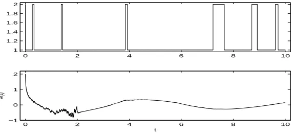
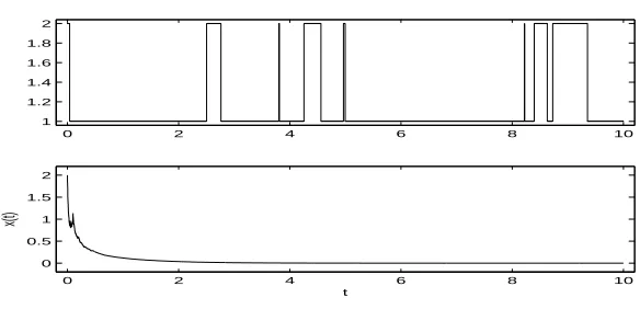
The above system (1.1) will switch from one mode to the other according to the probability law of the Markovian chain. Ifδ1(t)≤τ= 0.01, the computer simulation shows it is asymptotically stable (see Figure 4.1 ). If the time-delay is large, say

δ1(t)≤τ= 2, the computer simulation shows that the hybrid multiple-delays SDE (1.1) is unstable (see Figure 4.2 ). In other words, whether the hybrid multiple-delay SDE is stable or not depends on how small or large the time-multiple-delay is. On the other hand, both drift and diffusion coefficients of the hybrid SDE with multiple delays affect the stability of systems due to highly nonlinear. However, there is no delay dependent criterion which can be applied to the SDE with multiple delays to derive a sufficient bound on the time-delay τ such that the SDDE is stable, although the stability criteria of the highly nonlinear hybrid SDE with single delay have been created in [7]. This paper first established delay dependent criteria for highly nonlinear hybrid SDEs with variable multiple delays.

(3)

• This paper takes the variable multiple delays into account to develop a new theory on the robust stability and boundedness for highly nonlinear hybrid SDDEs.

• The new theory established in this paper is applicable to hybrid SDDEs with different delays in drift and diffusion coefficient of SDDEs with multiple delays (see (2.1)). Especially, we found that the sizes of delays in drift coefficient only affect the stability of the system, but the sizes of delays in the diffusion coefficient do NOT. This result has a significant importance.

• A significant amount of new mathematics has been developed to deal with the difficulties due to different delays in drift and diffusion coefficient of SD-DEs with multiple delays and those without the linear growth condition. For example, a more complicated Lyapunov function will be designed in order to deal with the effects of the different delays. A lot of effort has also been put into showing the bounds of the sizes of delays.

To develop our new theory, we will introduce some necessary notation in Section 2. We will discuss in Section 3 the delay-dependent asymptotic stability of SDEs with variable multiple delays, and give main results on robust boundedness and stability. We will present an example in Section 4 to illustrate our theory. We will ﬁnally conclude our paper in Section 5.

2. Notation and Assumptions

Throughout this paper, unless otherwise speciﬁed, we use the following notation. If

Ais a vector or matrix, its transpose is denoted by A⊤. Ifx∈Rd_{, then}_|_x_|_{is its} Euclidean norm. For a matrixA, we let|A|=√trace(A⊤A) be its trace norm and ∥A∥ = max{|Ax| : |x| = 1} be the operator norm. Let R+ = [0,∞). For τ > 0, denote by C([−τ,0];Rd_{) the family of continuous functions}_η _{from [}₋_τ,_0] _→ _Rd with the norm ∥η∥ = sup₋_τ_≤_u_≤₀|η(u)|. If A is a subset of Ω, denote by IA its indicator function. Let (Ω,F,{Ft}t≥0,P) be a complete probability space with a ﬁltration{Ft}t≥0 satisfying the usual conditions. LetB(t) = (B1(t),· · · , Bm(t))⊤ be anm-dimensional Brownian motion deﬁned on the probability space. Letr(t),

t≥0, be a right-continuous Markov chain on the probability space taking values in a ﬁnite state spaceS={1,2,· · ·, N}with generator Γ = (γij)N×N given by

P{r(t+ ∆) =j|r(t) =i}= {

γij∆ +o(∆) ifi̸=j, 1 +γii∆ +o(∆) ifi=j,

where ∆ > 0. Here γij ≥ 0 is the transition rate from i to j if i ̸= j while

γii = − ∑

j̸=iγij. We assume that the Markov chain r(·) is independent of the Brownian motion B(·). Let τj,¯δj ∈ [0,1), j = 1,· · · , n, be constants with τ =: maxn1

j=1τj. The delays δj(·) are diﬀerential functions fromR+ →[0, τ], such that ˙

δj(t) :=dδj(t)/dt≤δ¯j for allt≤0, andτj≥δj(t). For Borel measurable functions

f :Rd(n1+1)×S×R

+→Rd and g:Rd(n−n1+1)×S×R+→Rd×m, we consider ad-dimensional hybrid SDE withn-delays

(4)

+g(x(t), x(t−δn1+1(t)),· · ·, x(t−δn(t)), r(t), t)dB(t) (2.1)

ont≥0 with initial data

{x(t) :−τ≤t≤0}=η∈C([−τ,0];Rd), r(0) =i0∈S. (2.2)

The classical conditions for the existence and uniqueness of the global solution are the local Lipschitz condition and the linear growth condition (see, e.g., [24]). In this paper, we need only the local Lipschitz condition. However, we will con-sider highly nonlinear hybrid SDEs with multiple delays which, in general, do not satisfy the linear growth condition in this paper. Therefore, we impose the polyno-mial growth condition, instead of the linear growth condition. Let us state these conditions as an assumption for our aim.

Assumption 2.1. Assume that for anyh >0, there exists a positive constantKh such that

|f(x, y1,· · ·, yn1, i, t)−f(¯x,y¯1,· · ·,y¯n1, i, t)| ∨ |g(x, yn1+1,· · ·, yn, i, t)−g(¯x,y¯n1+1,· · ·,y¯n, i, t)|

≤Kh(|x−x¯|+ n ∑

j=1

|yj−y¯j|)

for allx, y1,· · · , yn,x,¯ y¯1,· · · ,y¯n∈Rdwith|x|∨|y1|∨· · ·∨|yn|∨· · ·∨|x¯|∨|y¯1|∨· · ·∨ |y¯n| ≤hand all (i, t)∈S×R+. Assume moreover that there exist three constants

K >0,q1≥1 andq2≥1 such that

|f(x, y1,· · ·, yn1, i, t)| ≤K(1 +|x| q1₊

n1 ∑

j=1 |yj|q1),

|g(x, yn1+1,· · ·, yn, i, t)| ≤K(1 +|x| q2₊

n ∑

j=n1+1

|yj|q2) (2.3)

for allx, y1,· · · , yn∈Rd,(i, t)∈S×R+.

If q1 = q2 = 1, then condition (2.3) is the familiar linear growth condition. However, we emphasise once again that we are here interested in highly nonlinear multiple-delay SDEs which have either q1 >1 or q2 >1. We will refer condition (2.3) as the polynomial growth condition. It is known that Assumption 2.1 only guarantees that the SDDE (2.1) with the initial data (2.2) has a unique maximal solution, which may explode to inﬁnity at a ﬁnite time. To avoid such a possible ex-plosion, we need to impose an additional condition in terms of Lyapunov functions. For this purpose, we need more notation.

LetC2,1₍_Rd_×_S_×_R_+;_R_{+) denote the family of non-negative functions}_U₍_{x, i, t}₎ deﬁned on (x, i, t)∈Rd_×_S_×_R

+ which are continuously twice diﬀerentiable in x and once int. For such a functionU(x, i, t), letUt= ∂U_∂t,Ux=

( ∂U ∂x1,· · ·,

∂U ∂xd

) , and

Uxx= (

∂2_U ∂xk∂xl

)

d_×d. LetC(R

d_×_[₋_τ,_∞_);_R_{+) denote the family of all continuous}

(5)

Assumption 2.2. Assume that there exists a pair of functions ¯U ∈C2,1₍_Rd_×_S_×

R+;R+) andG∈C(Rd_×_[₋_τ,_∞_);_R_{+), as well as positive numbers}_c

1, c2, c3,j and

q≥2(q1∨q2), such that n ∑

j=1

c3,j 1−δ¯j

< c2, |x|q≤U¯(x, i, t)≤G(x, t)

for∀(x, i, t)∈Rd_×_S_×_R_+, and

L_U¯₍_{x, y}₁_,_{· · ·}_{, y}_n_{, i, t}_{) := ¯}_U_t₍_{x, i, t}_{) + ¯}_U_x₍_{x, i, t}₎_f₍_{x, y}₁_,_{· · ·} _{, y}_n 1, i, t) +1

2trace[g T₍_{x, y}

n1+1,· · · , yn, i, t) ¯Uxx(x, i, t)g(x, yn1+1,· · ·,· · ·, yn, i, t)]

+ N ∑

j=1

γijU¯(x, j, t)

≤c1−c2G(x, t) + n ∑

j=1

c3,jG(yj, t−δj(t))

Similar to the discussion in [14], we have the following claim.

Lemma 2.1. Under Assumptions 2.1 and 2.2, the variable multiple-delay SDE (2.1) with the initial data (2.2) has the unique global solution x(t) on t≥ −τ and the solution has the property that

sup

−τ≤t<∞

E|x(t)|q<∞.

3. Delay-Dependent Asymptotic Stability of SDEs

with Variable Multiple Delays

In Lemma 2.1, we used the method of Lyapunov functions to study the existence and uniqueness of the solution of the highly nonlinear hybrid SDE (2.1). In this section, we will use the method of Lyapunov functionals to investigate the delay-dependent asymptotic stability. We deﬁne two segments ¯xt:={x(t+s) :−2τ ≤s≤0} and ¯

rt := {r(t+s) : −2τ ≤ s ≤ 0} for t ≥ 0. For ¯xt and ¯rt to be well deﬁned for 0≤t <2τ, we setx(s) =η(−τ) for s∈[−2τ,−τ) and r(s) =r0 fors∈[−2τ,0). We construct the Lyapunov functional as follows

V(¯xt,r¯t, t) =U(x(t), r(t), t)

+ n1 ∑

j=1

θj ∫ 0

−τj ∫ t

t+s [

τj|f(x(v), x(v−δ1(v)),· · · , x(v−δn1(v)), r(v), v)| 2

+|g(x(v), x(v−δn1+1(v)),· · ·, x(v−δn(v)), r(v), v)| 2]_dvds

fort≥0, whereU ∈C2,1(Rd×S×R+;R+) such that

lim

|x|→∞ [(t,i)inf∈R+×S

(6)

andθj, j= 1,· · ·, nare positive numbers to be determined later while we set

f(x, y1,· · ·, yn1, i, s) =f(x, y1,· · ·, yn1, i,0),

g(x, yn1+1,· · ·, yn, i, s) =g(x, yn1+1,· · · , yn, i,0)

for allx, y1,· · · , yn∈Rd,(i, s)∈S×[−2τ,0). Applying the generalized Itˆo formula (see, e.g., [26, Theorem 1.45 on page 48]) toU(x(t), r(t), t), we get

dU(x(t), r(t), t) = (

Ut(x(t), r(t), t)

+Ux(x(t), r(t), t)f(x(t), x(t−δ1(t)),· · ·, x(t−δn1(t)), r(t), t)

+1 2trace[g

T₍_x₍_t₎_{, x}₍_t₋_δ

n1+1(t)),· · · , x(t−δn(t)), r(t), t)

×Uxx(x(t), r(t), t)g(x(t), x(t−δn1+1(t)),· · ·, x(t−δn(t)), r(t), t)]

+ N ∑

j=1

γr(t),jU(x(t), j, t) )

dt+dM(t),

for t ≥0, where M(t) (see, e.g., [26, Theorem 1.45 on page 48]) is a continuous local martingale withM(0) = 0. Rearranging terms gives

dU(x(t), r(t), t)

= (

Ux(x(t), r(t), t)[f(x(t), x(t−δ1(t)),· · · , x(t−δn1(t)), r(t), t) −f(x(t), x(t),· · · , x(t), r(t), t)]

+LU(x(t), x(t−δn1+1(t)),· · · , x(t−δn(t)), r(t), t) )

+dM(t),

where the functionLU :Rd_×_Rd_×_S_×_R

+→Ris deﬁned by LU(x, yn1+1,· · ·, yn, i, t) =Ut(x, i, t) +Ux(x, i, t)f(x, x· · · , x, i, t)

+1 2trace[g

T₍_{x, y}

n1+1,· · ·, yn, i, t)Uxx(x, i, t)g(x, yn1+1,· · · , yn, i, t)] + N ∑

j=1

γijU(x, j, t).

(3.1)

Moreover, the fundamental theory of calculus shows, forj= 1,· · · , n,

d

( ∫ 0

−τj ∫ t

t+s [

+|g(x(v), x(v−δn1+1(v)),· · ·, x(v−δn(v)), r(v), v)|

2]_dvds)

= (

τj [

τj|f(x(t), x(t−δ1(v)),· · · , x(t−δn1(v)), r(t), t)| 2

+|g(x(t), x(t−δn1+1(v)),· · · , x(t−δn(v)), r(t), t)| 2]

− ∫ t

t−τj [

(7)

Lemma 3.1. With the notation above,V(¯xt,r¯t, t) is an Itˆo process on t≥0 with

its Itˆo diﬀerential

dV(¯xt,¯rt, t) =LV(¯xt,¯rt, t)dt+dM(t),

whereM(t)is a continuous local martingale withM(0) = 0and

LV(¯xt,¯rt, t) =Ux(x(t), r(t), t)[f(x(t), x(t−δ1(t)),· · · , x(t−δn1(t)), r(t), t) −f(x(t), x(t),· · ·, x(t), r(t), t)]

+LU(x(t), x(t−δ1(t)),· · ·, x(t−δn(t)), r(t), t)

+ n1 ∑

j=1

θjτj [

τj|f(x(t), x(t−δ1(t)),· · ·, x(t−δn1(t)), r(t), t)| 2

+|g(x(t), x(t−δn1+1(t)),· · ·, x(t−δn(t)), r(t), t)| 2]

− n1 ∑

j=1

θj ∫ t

t₋τj [

τj|f(x(v), x(v−δ1(v)),· · ·, x(v−δn1(v)), r(v), v)| 2

+|g(x(v), x(v−δn1+1(v)),· · ·, x(v−δn(v)), r(v), v)| 2]_dv.

To study the delay-dependent asymptotic stability of the SDDE (2.1), we need to impose several new assumptions.

Assumption 3.1. Assume that there are functionsU ∈ C2,1₍_Rd_×_S_×_R +;R+),

U1 ∈ C(Rd ×[−τ,∞);R+), and positive numbers α, αj (j = 1,· · ·, n) and βk (k= 1,2,3) such that

n ∑

j=1

αj 1−¯δj

< α (3.2)

and

LU(x, y1,· · · , yn, i, t) +β1|Ux(x, i, t)|2 +β2|f(x, y1,· · ·, yn1, i, t)|

2₊_β_3|_g₍_{x, y}

n1+1,· · ·, yn, i, t)| 2

≤ −αU1(x, t) + n ∑

j=1

αjU1(yj, t−δj(t)), (3.3)

Assumption 3.2. Assume that there exists positive numberswj, j= 1,· · · , nsuch that

|f(x, x,· · · , x, i, t)−f(x, y1,· · ·, yn1, i, t)| ≤ n1 ∑

j=1

wj|x−yj|

for allx, y1· · · , yn∈Rd,(i, t)∈S×[−2τ,∞).

Theorem 3.3. Let Assumptions 2.1, 2.2, 3.1 and 3.2 hold. Assume also that

n1 n1 ∑

j=1

w2_jτ_j2≤2β1β2 and n1 n1 ∑

j=1

(8)

Then for any given initial data (2.2), the solution of the SDDE (2.1) has the

prop-erties that _∫

∞

0

EU1(x(t), t)dt <∞ (3.5)

and

sup 0≤t<∞

EU(x(t), r(t), t)<∞.

Proof: Fix the initial dataη∈C([−τ,0];Rd_{) and}_r

0∈Sarbitrarily. Letk0>0 be a suﬃciently large integer such that∥η∥:= sup₋_τ_≤_s_≤₀|η(s)|< k0. For each integer

k > k0, deﬁne the stopping time

σk = inf{t≥0 :|x(t)| ≥k},

where throughout this paper we set infϕ=∞(as usual ϕdenotes the empty set). It is easy to see thatσk is increasing as k→ ∞ and limk_→∞σk =∞ a.s. By the generalized Itˆo formula we obtain from Lemma 3.1 that

EV(¯xt∧σk,r¯t∧σk, t∧σk) =V(¯x0,r¯0,0) +E ∫ t∧σk

0

LV(¯xs,r¯s, s)ds (3.6)

for anyt≥0 andk≥k0. Letθj =n1wj2/(2β1). By Assumption 3.2, it is easy to see that

Ux(x(t), r(t), t)[f(x(t), x(t−δ1(t)),· · ·, x(t−δn1(t)), r(t), t) −f(x(t), x(t),· · ·, x(t), r(t), t)]

≤β1|Ux(x(t), r(t), t)|2+n1 n1 ∑

j=1

w2_j

4β1|

x(t)−x(t−δj(t))|2. (3.7)

By condition (3.4), we also have

n1 ∑

j=1

θjτj2≤β2 and n1 ∑

j=1

θjτj≤β3.

It then follows from Lemma 3.1 that

LV(¯xs,r¯s, s)≤ LU(x(s), x(s−δ1(s)),· · ·, x(t−δn(s)), r(s), s) +β1|Ux(x(s), r(s), s)|2 +β2|f(x(s), x(s−δ1(s)),· · ·, x(t−δn1(s)), r(s), s)|

2

+β3|g(x(s), x(s−δn1+1(s)),· · · , x(t−δn(s)), r(s), s)| 2

+n1 n1 ∑

j=1

w2 j 4β1

|x(s)−x(s−δj(s))|2

−n1 n1 ∑

j=1

w2 j 2β1

∫ s

s−τj [

(9)

By Assumption 3.1, we then have

LV(¯xs,¯rs, s)≤ −αU1(x(s), s) + n ∑

j=1

αjU1(x(s−δj(s)), s−δj(s))

+n1 n1 ∑

j=1

w2_j

4β1|

x(s)−x(s−δj(s))|2

−n1 n1 ∑

j=1

w2_j

2β1 ∫ s

s−τj [

+|g(x(v), x(v−δn1+1(v)),· · ·, x(v−δn(v)), r(v), v)| 2]_dv.

Substituting this into (3.6) implies

EV(¯xt∧σk,¯rt∧σk, t∧σk)≤V(¯x0,r¯0,0) +H1+ n1 ∑

j=1

(H₂j−H₃j), (3.8)

where

H1=E ∫ t∧σk

0 [

−αU1(x(s), s) + n ∑

l=1

αlU1(x(s−δl(s)), s−δl(s)) ]

ds,

H₂j= n1w 2 j 4β1

E

∫ t_∧σk

0

|x(s)−x(s−δj(s))|2ds,

H₃j= n1w 2 j 2β1 E

∫ t∧σk

0 ∫ s

s₋τj [

+|g(x(v), x(v−δn1+1(v)),· · · , x(v−δn(v)), r(v), v)| 2]_dvds.

Noting that, forl= 1,· · · , n,

∫ t∧σk

0

U1(x(s−δl(s)), s−δl(s))ds≤

∫ t∧σk−δl(t∧σk)

−δl(0)

U1(x(v), v) 1−δ¯l

dv≤

∫ t∧σk

−τl

U1(x(v), v) 1−¯δl

dv,

we have

H1≤ n ∑

l=1

αl 1−¯δl

∫ 0

−τl

U1(η(v), v)dv−α¯E ∫ t∧σk

0

U1(x(s), s)ds,

where ¯α=α−

n ∑ l=1

αl/(1−δ¯l)>0 by Assumption 3.1. Substituting this into (3.8) yields

¯

αE

∫ t_∧σk

0

U1(x(s), s)ds≤C1+ n1 ∑

j=1

(H₂j−H₃j), (3.9)

whereC1is a constant deﬁned by

C1=V(¯x0,¯r0,0) + n ∑

l=1

αl 1−δ¯l

∫ 0

−τl

(10)

Applying the classical Fatou lemma and letk→ ∞in (3.9) to obtain

¯

αE

∫ t

0

U1(x(s), s)ds≤C1+ n1 ∑

j=1

( ¯H₂j−H¯₃j), (3.10)

where

¯

H₂j =n1w 2 j 4β1 E

∫ t

0

|x(s)−x(s−δj(s))|2ds,

¯

H₃j =n1w 2 j 2β1 E

∫ t

0 ∫ s

s−τj [

2]_dvds. _(3.11)

By the well-known Fubini theorem, we have

¯

H₂j =n1w 2 j 4β1

∫ t

0

E|x(s)−x(s−δj(s))|2ds.

Fort∈[0, τj], we have

¯

H₂j≤ n1w

2 j 2β1

∫ τj

0

(E|x(s)|2+E|x(s−δj(s))|2)ds

≤ n1w 2 jτj

β1 (

sup

−τj≤v≤τj

E|x(v)|2 )

≤ n1wj2τj

β1 (

sup

−τ≤v≤τ

E|x(v)|2 )

.

Fort > τj, we have

¯

H₂j ≤n1w

2 jτj

β1 (

sup

−τ≤v≤τ

E|x(v)|2 )

+n1w 2 j 4β1

∫ t

τj

E|x(s)−x(s−δj(s))|2ds. (3.12)

Noting that

|x(s)−x(s−δj(s))|

≤ | ∫ s

s−τj

f(x(v), x(v−δ1(v)),· · · , x(v−δn1(v)), r(v), v)dv

+ ∫ s

s−τj

g(x(v), x(v−δn1+1(v)),· · ·, x(v−δn(v)), r(v), v)dB(v)|,

we have

E|x(s)−x(s−δj(s))|2

≤2E ∫ s

s−τj

[τj|f(x(v), x(v−δ1(v)),· · ·, x(v−δn1(v)), r(v), v)| 2

(11)

Notice also that ∫ t

τj

E|x(s)−x(s−δj(s))|2

≤2E ∫ t

τj ∫ s

s₋τj

[τj|f(x(v), x(v−δ1(v)),· · ·, x(v−δn1(v)), r(v), v| 2

+|g(x(v), x(v−δn1+1(v)),· · · , x(v−δn(v)), r(v), v)| 2_]_dvds.

Thus from (3.11) and (3.12) we get

¯

H₂j≤ n1w

2 jτj

β1 (

sup

−τ≤v≤τ

E|x(v)|2 )

+ ¯H₃j. (3.13)

Substituting (3.13) into (3.10) yields

¯

αE

∫ t

0

U1(x(s), s)ds≤C1+ 2β3 sup

−τ_≤v_≤τE|

x(v)|2:=C2.

Lettingt→ ∞gives

E

∫ _∞

0

U1(x(s), s)ds≤C2

¯

α. (3.14)

Now we see from (3.8) that

EU

(

x(t∧σk), r(t∧σk), t∧σk )

≤C1+ n1 ∑

j=1

(H₂j−H₃j). (3.15)

Lettingk→ ∞we get

EU(x(t), r(t), t)≤C2<∞,

which shows

sup 0≤t<∞E

U(x(t), r(t), t)<∞. (3.16)

Thus the proof is complete. 2

Corollary 3.1. Let the conditions of Theorem 3.3 hold. If there moreover exists a pair of positive constantscandpsuch that

c|x|p≤U1(x, t), ∀(x, t)∈Rd×R+,

then for any given initial data (2.2), the solution of the multiple-delay SDE (2.1) satisﬁes

∫ _∞

0

E|x(t)|pdt <∞. (3.17)

That is, the multiple-delay SDE (2.1) isH_∞-stable inLp_.

(12)

Theorem 3.4. Let the conditions of Corollary 3.1 hold. If, moreover,

p≥2 and (p+q1−1)∨(p+ 2q2−2)≤q,

then the solution of the multiple-delay SDE (2.1) satisﬁes

lim t→∞E|x(t)|

p_{= 0}

for any initial data (2.2). That is, the variable multiple-delay SDE (2.1) is asymp-totically stable inLp_.

Proof: Fix the initial data (2.2) arbitrarily. For any 0≤t1< t2<∞, by the Itˆo formula, we get

E|x(t2)|p−E|x(t1)|p

=E ∫ t2

t1 (

p|x(t)|p−2x(t)⊤f(x(t), x(t−δ1(t)),· · ·, x(t−δn1(t)), r(t), t)

+p 2|x(t)|

p−2_|_g₍_x₍_t₎_{, x}₍_t₋_δ

n1+1(t)),· · ·, x(t−δn(t)), r(t), t)| 2

+p(p−2) 2 |x(t)|

p₋4_|₍_x₍_t₎_⊤_g₍_x₍_t₎_{, x}₍_t₋_δ

n1+1(t)),· · ·, x(t−δn(t)), r(t), t)| 2)_dt,

which implies

_E_|x(t2)|p−E|x(t1)|p

≤E

∫ t2

t1 (

p|x(t)|p−1|f(x(t), x(t−δ1(t)),· · ·, x(t−δn1(t)), r(t), t)|

+p(p−1) 2 |x(t)|

p₋2_|_g₍_x₍_t₎_{, x}₍_t₋_δ

n1+1(t)),· · ·, x(t−δn(t)), r(t), t)| 2)_dt

≤E

∫ t2

t1 (

pK|x(t)|p−1[1 +|x(t)|q1₊ n1 ∑

j=1

|x(t−δj(t))|q1 ]

+(n−n1+ 2)p(p−1)K 2

2 |x(t)|

p₋2[_{1 +}_|_x₍_t₎_|2q2₊ n ∑

j=n1+1

|x(t−δj(t))|2q2 ])

dt.

By inequalities,

|x(t)|p−1|x(t−δj(t))|q1 ≤ |x(t)|p+q1−1+|x(t−δj(t))|p+q1−1, |x(t)|p−1≤1 +|x(t)|q,

we can obtain

_E_|x(t2)|p−E|x(t1)|p≤C3(t2−t1), where

C3=pK(1 + 2(n1+ 1) sup

−τ≤t<∞E|

x(t)|q)

+1

2(n−n1+ 2)p(p−1)K

2_{(1 + 2(}_n₋_n

1+ 1) sup

−τ≤t<∞

E|x(t)|q)<∞.

(13)

4. An Example for Muptiple-delay SDEs

Let us now discuss an example to illustrate our theory.

Example 4.1. Let us consider the SDDE with two delays (1.1), we consider two case: δ1(t) ≤ τ = 0.01 and δ1(t) ≤ τ = 2 for all t ≥ 0. Let ¯δ1 = ¯δ2 = 0.1 and

δ2(t) = 2 (in fact, the stability of system is independent on the size of δ2(t)). In caseτ = 0.01, let the initial datax(u) = 2 + sin(u) foru∈[−0.01,0], r(0) = 2, the sample paths of the Markovian chain and the solution of the multiple delay SDE are shown in Figure 4.1, which indicates that the multiple delay SDE is asymptotically stable. In the case τ = 2, let the initial data x(u) = 2 + sin(u) for u ∈ [−2,0], r(0) = 2, the sample paths of the Markovian chain and the solution of the multiple-delay SDE are plotted in Figure 4.2, which indicates that the multiple-multiple-delay SDE is asymptotically unstable. From the example we can see SDDE (1.1) is stable or not depends on how long or short the time-delay is.

0 2 4 6 8 10

1 1.2 1.4 1.6 1.8 2

0 2 4 6 8 10

−1 0 1 2

t

[image:13.612.148.434.282.415.2]

x(t)

Figure 4.1: The computer simulation of the sample paths of the Markovian chain and the SDDE (1.1) withτ = 0.01 using the Euler–Maruyama method with step size 10−3.

0 2 4 6 8 10

1 1.2 1.4 1.6 1.8 2

0 2 4 6 8 10

−1 0 1 2

t

x(t)

[image:13.612.149.435.497.630.2]

(14)

We can see coeﬃcients deﬁned by (1.1) satisfy Assumption 2.1 withq1= 3 and

q2= 2. Deﬁne ¯U(x, i, t) =|x|6 for (x, i, t)∈R×S×R+. It is easy to show that

L_U¯₍_{x, y}₁_{, y}₂_{, i, t}_{) = 6}_x5_f₍_{x, y}

1, i, t) + 15x4|g(x, y2, i, t)|2 for (x, y1, y2, i, t)∈R3×S×R+. We have

L_U¯₍_{x, y}₁_{, y}₂_,₁_{, t}_{) =6}_x5₍₋_y

1−10x3) + 15 16x

4₍1 4y

2 2)

2

≤5x6+y₁6+ 15 128y

6

2−(60− 15 128)x

8

and

L_U¯₍_{x, y}₁_{, y}₂_,₂_{, t}_{) =6}_x5₍1

2y1−4x 3_{) +}15

4 x 4₍_y2

2) 2

≤2.5x6+ 0.5y₁6−22.125x8+ 1.875y₂8.

Thus, we can obtain

L_U¯₍_{x, y}

1, y2, i, t)≤5x6+y16−22.125x

8_{+ 1}_.₈₇₅_y8 2 ≤c1−10(1 +x8) + (1 +y81) + 2(1 +y

8 2), where

c1= sup x_∈_R{

8 + 5x6−12.125x8}<∞

and G(x, t) = 1 +x8_{, c}

2 = 10, c3,1 = 1, c3,2 = 2. Therefore, Assumption 2.2 is satisﬁed. From Lemma 2.1, solution of the SDDE (1.1) has the that

sup

−τ≤t<∞E|

x(t)|6<∞.

To verify Assumption 3.1, we deﬁne

U(x, i, t) =   

x2₊_x4_, _if_i_{= 1}_, 2x2+ 3x4, ifi= 2

(4.1)

which shows

Ux(x, i, t) =   

2x+ 4x3_, _if_i_{= 1}_, 4x+ 12x3_, _if_i_{= 2}

for (x, i, t)∈R×S×R+. By the equation (3.1), we have

LU(x, y2,1, t) =(2x+ 4x3)(−x−10x3) + 1 32(y

2 2)

2_{(2 + 12}_x2₎₋₍_x2₊_x4_{) + (2}_x2_{+ 3}_x4₎

≤ −x2−22x4−39.875x6+ 1 16y

4

2+ 0.25y 6 2

and

LU(x, y2,2, t) =(4x+ 12x3)( 1 2x−4x

3_{) +}1 8(y

2 2)

(15)

≤ −6x2−26x4−46.5x6+1 2y

4 2+ 3y

6 2.

Moreover

|Ux(x, i, t)|2=   

4x2_{+ 16}_x4_{+ 16}_x6_, _if_i_{= 1}_,

16x2_{+ 96}_x4_{+ 144}_x6_,_if_i_{= 2}_. (4.2)

|f(x, y1, i, t)|2=   

| −y1−10x3|2≤2y21+ 200x

6_,_if_i_{= 1}_, |1

2y1−4x 3_|2_≤ 1

2y 2 1+ 32x

6_, _if_i_{= 2}_. (4.3)

|g(x, y2,1, t)|2=   

1 16|y

2

2|2_,_if_i_{= 1}_, 1

4|y 2

2|2, ifi= 2.

(4.4)

Settingβ1= 0.05,β2= 0.1,β3= 4, using (4.2)-(4.4), we obtain that

LU(x, y1, y2, i, t) +β1|Ux(x, i, t)|2+β2|f(x, y1, y2, i, t)|2+β3|g(x, y1, y2, i, t)|2

≤   

−0.8x2₋₂₁_.₂_x4₋₁₉_.₀₇₅_x6_{+ 0}_.₂_y2 1+165y

4 2+14y

6

2, ifi= 1, −5.2x2₋₂₁_.₁_x4₋₃₆_.₁_x6_{+ 0}_.₀₅_y2

1+ 1.5y42+ 3y62, ifi= 2. This implies

4 + 3y6

≤ −6(0.1x2+ 3x4+ 3x6) + 2(0.1y₁2+ 3y₁4+ 3y6₁) + 0.1y₂2+ 3y4₂+ 3y₂6.

LettingU1(x, t) = 0.1x2_{+ 3}_x4_{+ 3}_x6_,_α_{= 6,}_α

1= 2, α2= 1,, we get condition (3.2). Noting thatn1= 1, n= 2 and w1= 1, then condition (3.4) becomes

τ ≤0.1

By Theorem 3.3, we can therefore conclude that the solution of the SDDE (1.1) has the properties that

∫ _∞

0

(x2(t) +x4(t) +x6(t))dt <∞a.s. and ∫ _∞

0

E(x2(t) +x4(t) +x6(t))dt <∞.

Moreover, as|x(t)|p≤x2(t) +x4(t) +x6(t) for anyp∈[2,6], we have ∫ _∞

0

E|x(t)|pdt <∞.

Recallingq1= 3, q2= 2 andq= 6, we see that forp= 4, all conditions of Theorem 3.4 are satisﬁed and hence we have

lim t→∞E|x(t)|

4 = 0.

(16)

0 2 4 6 8 10 1

1.2 1.4 1.6 1.8 2

0 2 4 6 8 10

0 0.5 1 1.5 2

t

[image:16.612.143.435.86.227.2]

x(t)

Figure 4.3 : The computer simulation of the sample paths of the Markovian chain and the SDDE (1.1) withτ= 0.1 using the Euler–Maruyama method with step size 10−3.

5. Conclusion

In real world applications, the stability and boundedness of stochastic differential delay equations are interesting topics. In this paper, we established the criteria of stability and boundedness of the solutions to SDDEs with variable multiple delays. To this end, we investigated the highly nonlinear hybrid multiple-delay SDEs. In fact, the stability of SDDEs have been studied for many years, most of the results in this topic require that the coefficients of equations are linear or nonlinear but bounded by linear functions. Recently, without the linear growth condition, Fei et al. [7] was the first to establish the delay-dependent stability criteria for highly nonlinear SDDEs by the method of Lyapunov function with a single time delay. In this paper, we obtained the results of hybrid highly nonlinear SDE with variable multiple delays. An illustrative example was given for our theory.

References

[1] A. Ahlborn and U. Parlitz, Stabilizing unstable steady states using multiple delay feedback control, Phys. Rev. Lett., 2014, 93, 264101.

[2] C. Briat, Stability analysis and stabilization of stochastic linear impulsive, switched and sampled-data systems under dwell-time constraints, Automatica, 2016, 74, 279–287.

[3] H. B. Chen, P. Shi and C. Lim, Stability analysis for neutral stochastic delay systems with Markovian switching, Syst. Control Lett., 2017, 110, 38–48. [4] V. Dragan and H. Mukaidani, Exponential stability in mean square of a

sin-gularly perturbed linear stochastic system with state-multiplicative white-noise perturbations and Markovian switching, IET Control Theory Appl., 2016, 9, 1040–1051.

(17)

[6] C. Fei, M. X. Shen, W. Y. Fei, X. R. Mao and L. T. Yan, Stability of highly nonlinear hybrid stochastic integro-diﬀerential delay equations, Nonlinear Anal. Hybrid Syst., 2019, 31, 180–199.

[7] W. Y. Fei, L. J. Hu, X. M. Mao and M. X. Shen,Delay dependent stability of highly nonlinear hybrid stochastic systems, Automatica, 2017, 28, 165–170. [8] W. Y. Fei, L. J. Hu, X. R. Mao and M. X. Shen, Structured robust stability

and boundedness of nonlinear hybrid delay systems, SIAM J. Control Optim., 2018, 56, 2662–2689.

[9] W. Y. Fei, L. J. Hu, X. R. Mao and M. X. Shen,Generalised criteria on delay dependent stability of highly nonlinear hybrid stochastic systems, Int. J. Robust. Nonlin., DOI: 10.1002/rnc.4402.

[10] M. Frederic,Stability analysis of time-varying neutral time-delay systems, IEEE Trans. Automat. Control, 2016, 60, 540–546.

[11] E. Fridman, Introduction to Time-Delay Systems: Analysis and Control, Birkhauser, 2014.

[12] A. Garab, V. Kovcs and T. Krisztin Global stability of a price model with multiple delays, Discrete Contin. Dyn. Syst. A., 2016,36(12),6855C6871. [13] J. K. Hale and S. M. Lunel,Introduction to Functional Diﬀerential Equations,

Springer-Verlag, 1993.

[14] L. J. Hu, X. R. Mao and Y. Shen,Stability and boundedness of nonlinear hybrid stochastic diﬀerential delay equations, Syst. Control Lett., 2013, 62, 178–187. [15] L. J. Hu, X. R. Mao and L. G. Zhang, Robust stability and boundedness of

nonlinear hybrid stochastic delay equations, IEEE Trans. Automat Control, 2013, 58(9), 2319–2332.

[16] V. B. Kolmanovskii and V. R. Nosov, Stability of Functional Diﬀerential E-quations, Academic Press, London, 1986.

[17] M. L. Li and M. C. Huang,Approximate controllability of second-order impul-sive stochastic diﬀerential equations with state-dependent delay, J. Appl. Anal. Comput., 2018, 8(2), 598–619.

[18] X. D. Li, Q. X. Zhu and D. O’Reganc, pth Moment exponential stability of impulsive stochastic functional diﬀerential equations and application to control problems of NNs, J. Franklin Inst., 2014, 351, 4435–4456.

[19] J. Lei and M. Mackey,Stochastic diﬀerential delay equation, moment stability, and application to hematopoitic stem cell regulation systems, SIAM J. Appl. Math., 2007, 67(2), 387–407.

[20] J. Liu,On asymptotic convergence and boundedness of stochastic systems with time-delay, Automatica, 2012, 48, 3166–3172.

[21] K. Liu, Almost sure exponential stability sensitive to small time delay of s-tochastic neutral functional diﬀerential equations, Appl. Math. Lett., 2018, 77, 57–63.

[22] X. R. Mao, Razumikhin-type theorems on exponential stability of stochastic functional diﬀerential eqautions, Stoch. Process. Appl., 1996, 65, 233-250. [23] X. R. Mao, Exponential stability of stochastic delay interval systems with

(18)

[24] X. R. Mao,Stochastic Diﬀerential Equations and Their Applications, 2nd Edi-tion, Chichester: Horwood Pub., 2007.

[25] X. R. Mao, J. Lam, and L. R. Huang, Stabilisation of hybrid stochastic d-iﬀerential equations by delay feedback control, Syst. Control Lett., 2008, 57, 927–935.

[26] X. R. Mao and C. G. Yuan,Stochastic Diﬀerential Equations with Markovian Switching, Imperial College Press, 2006.

[27] S.-E.A. Mohammed, Stochastic Functional Diﬀerential Equations, Longman Scientiﬁc and Technical, 1984.

[28] C. Park, N. Kwon and P. Park,Optimal H_∞ ﬁltering for singular Markovian jump systems, Syst. Control Lett., 2018, 118, 22–28.

[29] A. Rathinasamy and M. Balachandran,Mean-square stability of semi-implicit Euler method for linear stochastic diﬀerential equations with multiple delays and Markovian switching, Appl. Math. Comput., 2008, 206, 968–979.

[30] M. X. Shen, C. Fei, W. Y. Fei and X. R. Mao,The boundedness and stability of highly nonlinear hybrid neutral stochastic systems with multiple delays, Sci. China Inf. Sci., revised.

[31] M. X. Shen, W. Y. Fei, X. R. Mao and S. N. Deng, Exponential stability of highly nonlinear neutral pantograph stochastic diﬀerential equations, Asian J. Control, DOI: 10.1002/asjc.1903.

[32] M. X. Shen, W. Y. Fei, X. R. Mao and Y. Liang,Stability of highly nonlinear neutral stochastic diﬀerential delay equations, Syst. Control Lett., 2018, 115, 1–8.

[33] S. Y. Xu, J. Lam and X. R. Mao, Delay-dependent H_∞ control and ﬁltering for uncertain Markovian jump systems with time-varying delays, IEEE Trans. Circuits Syst. I, 2007, 54(9), 2070–2077.

[34] S. R. You, W. Liu, J. Q. Lu, X. R. Mao and J. W. Qiu,Stablization of hybrid systems by feedback control based on discrete-time state observation, SIAM J. Contrl Optim., 2015, 53(2), 905–925.

[35] D. Yue and Q. Han,Delay-dependent exponential stability of stochastic systems with time-varying delay, nonlinearity, and Markovian switching, IEEE Trans. Automat. Control, 2005, 50, 217–222.