Scale robust IMU-assisted KLT for stereo visual odometry solution

City, University of London Institutional Repository

Citation

:

(2017). Scale robust IMU-assisted KLT for stereo visual odometry solution. Robotica, 35(9), pp. 1864-1887. doi: 10.1017/S0263574716000552

This is the published version of the paper.

This version of the publication may differ from the final published

version.

Permanent repository link: http://openaccess.city.ac.uk/22087/

Link to published version

:

Copyright and reuse:

City Research Online aims to make research

outputs of City, University of London available to a wider audience.

Copyright and Moral Rights remain with the author(s) and/or copyright

holders. URLs from City Research Online may be freely distributed and

linked to.

Robotica: page 1 of 24. © Cambridge University Press 2016 doi:10.1017/S0263574716000552

Scale robust IMU-assisted KLT for stereo visual

odometry solution

L. Chermak

∗

, N. Aouf and M. A. Richardson

Centre of Electronic Warfare, Cranfield University, Shrivenham, SN6 8LA, UK E-mails: [email protected], [email protected]

(Accepted July 23, 2016)

SUMMARY

We propose a novel stereo visual IMU-assisted (Inertial Measurement Unit) technique that extends to large inter-frame motion the use of KLT tracker (Kanade–Lucas–Tomasi). The constrained and coherent inter-frame motion acquired from the IMU is applied to detected features through homogenous transform using 3D geometry and stereoscopy properties. This predicts efficiently the projection of the optical flow in subsequent images. Accurate adaptive tracking windows limit tracking areas resulting in a minimum of lost features and also prevent tracking of dynamic objects. This new feature tracking approach is adopted as part of a fast and robust visual odometry algorithm based on double dogleg trust region method. Comparisons with gyro-aided KLT and variants approaches show that our technique is able to maintain minimum loss of features and low computational cost even on image sequences presenting important scale change. Visual odometry solution based on this IMU-assisted KLT gives more accurate result than INS/GPS solution for trajectory generation in certain context.

KEYWORDS: Computer vision, Navigation, IMU-KLT feature tracking, Visual odometry, Double dogleg.

1. Introduction

The process of estimating camera motion from the analysis of feature correspondences within a sequence of images over time is called visual odometry (VO).1_{In recent years, many research works}

have contributed to the success and establishment of this methodology.2−5_{VO does not necessarily}

use computer vision techniques only. Indeed, improvement, assistance, or fusion to visual processing techniques using sensors such as an IMU (Inertial Measurement Unit) or a GPS (Global Positioning System) have a positively contributed to VO solutions. This work concentrates on feature tracking in a VO context. Accurate estimation of the camera motion during navigation depends on the ability to successfully track features over successive images. KLT (Kanade–Lucas–Tomasi) is one of the most popular features tracking technique.6−8 KLT considers local information derived from small search windows surrounding each of the interest points. This local process constrains template image analysis in time, space, and brightness. This is acceptable for image sequences with small appearance change i.e., high frame rate, coherent motion, stable illumination, etc. As a consequence, it is relatively efficient on image sequences with small changes in appearance between subsequent frames. However, it becomes very difficult and sometimes impossible for KLT tracker to deal with large inter-frame motions inducing a substantial optical flow. In order to deal with this problem, a pyramidal implementation of the KLT algorithm was developed.9_{The latter runs the KLT algorithm}

iteratively on a local template window through successive multi-resolution layers starting from the top of the pyramid (lowest resolution) until recovering the initial image size. This allows larger motions to be caught with less difficulty by breaking the distance through this multi-scale approach. Although it is reasonably efficient, it also implies a certain computational cost which makes its use difficult for

real-time applications, especially in VO context where feature tracking is just a stage among others in the VO pipeline.

In general, the majority of KLT-based variants modify the warping function using an affine model to adapt the template to the different conditions that might occur between two successive images, such as change in illumination, rotation, and scale.10−12 _{The work of Hwangbo}13 _{presents a}

gyro-aided KLT method. The instantaneous gyro angles are used to get inter-image rotation that serves to compute the homography matrix between two consecutive images.

The obtained homography matrix is used to update the parameters of an affine photometric model for the warping function. The affine photometric model has eight parameters allowing robust tracking to camera rotation and outdoor illumination. However, this model leads to a significant computational cost.

Another work14 proposes a gyro-aided feature tracking solution for video stabilization. In this contribution, gyroscope measurements from IMU sensor and intrinsic camera parameters are also used to obtain the homography matrix. In contrast to Hwangbo,13for computation complexity reasons a translational model is preferred to the affine one for the KLT warping function. While these two precedent works are mono-camera-based approaches,13,14 Tanathong15 presents a stereo-camera-based approach. In this work, stereo cameras are mounted on a UAV, and GPS/INS subsequent position information are used to determine the rotation angle of stereo rig between these two positions. Two affine models for warping function using orientation information are proposed here. Assuming a constant distance between the UAV and the ground (i.e., camera facing the ground with no scale changes), the angular information is either used to rotate the entire current images into the same orientation as the previous images; or to rotate the tracking windows into the same orientation as the previous images. Feature tracking is based on pyramidal KLT.

In these three contributions,13−15 _{the benefit of gyroscope information is significant allowing}

the KLT to cope with sharp rotation where it usually fails. However, this remains possible only at the condition of a quasi-pure or a pure camera rotation. Hence, it is assumed a negligible inter-frame translation regarding the scene depth (i.e., very small scale change). High inter-frame rate enables to fulfil this condition, and can be easily achieved due to computational efficiency of the KLT translational model.14,15 On the other hand, the approach used by Hwangbo13 requires a parallel processing implementation to achieve high frame rate. Also, by using GPS/INS, the method proposed by Tanathong15is still dependent from an external source of information.

Our motivation is to propose an innovative and computationally efficient IMU-assisted KLT tracker, using the full IMU information; robust against rotation changes similarly as13−15 _{but also}

against important scaling between consecutive images. This allows the KLT to be partially released of its spatial constraint allowing low frame rate processing, which is not the case for gyro-only solutions. To enable a continuous and efficient use of accelerometer measurements, the IMU information has to be updated over time. This is why our IMU-assisted KLT tracker technique is an integral part of a VO algorithm, which is the second contribution of this work. Indeed, at each new image the inter-frame pose resulting from our VO initialises the IMU. The overall solution is independent of any external source (e.g., GPS).

This paper is organized as follows: Section 2 describes the overall VO algorithm. Section 3 focuses on IMU-assisted feature tracking and adaptive local tracking window concept. Section 4 gives the detail of double dogleg (DDL) algorithm for motion estimation. Results and discussion are presented in Section 5. Finally, we draw conclusions.

2. System Overview

2.1. Visual odometry and IMU association

Limitations of classical VO have been well identified in the literature.16Hence, many fusion works with various sensors have been investigated in order to find the most complementary combination. IMU is particularly cheap and easy to implement with vision system. Its high frequency provides precious motion information filling the interval gap of lower frequency associated vision sensors.17−19

It is well known that inertial measurements drift with time if there is no update from an external source.20 _{Associating it with sensors such as GPS or camera(s), allows the correction of the IMU}

IMU initialisation

Inertial acquisition and

Integration

Generation of the initial features

-Feature Detection -Stereo Matching

-3D reconstruction _2D

Projection

Generation of the final features

-Adaptive Local Search Window

-IMU-KLT Feature Tracking

Visual Ego-Motion

+

Absolute Pose

{ Rimu, timu }

{ sp, Sp} { s*c, S*c}

{ sp, s*c, d, dcr }

{ sp, Sc}

{ϕimu, θimu, ψimu}

{ tv}

{ Rv, tv}

time

t+1 t

Previous stereo pair _{Current stereo pair}

IMU Vision only IMU only Combined data

{ R(qimu0),timu0}

{ R, t }

Fig. 1. Illustration of IMU-assisted feature tracking principle in the visual odometry framework.

provide the gravity vector, resulting in a reduction of motion parameters.21_{Those are then combined}

with Hough Transform to estimate the ego-motion without feature correspondence.

The use of an Extended Kalman Filter (EKF) or one of it variants has been favoured and extensively employed to fuse inertial and vision data, essentially to resolve pose estimation problem.22−24_Despite

showing relatively good efficiency, Kalman Filter approaches based on the pinhole camera model involve costly update of the covariance matrix. This is especially the case for the ones including features in the state vector.

The novel VO approach proposed here is not a pure fusion, but more a complementary association with the IMU. VO benefits from a better quality of features with the IMU-assisted KLT, whilst the IMU is initialised from visual motion estimation. Our approach aims to handle large motion and computational burden by exploiting high-frequency measurements from the IMU.

2.2. Algorithm description

Figure 1 illustrates the whole framework of our VO algorithm, which includes IMU-assisted KLT feature tracking. The different stages composing the algorithm are divided into three categories: Vision only, IMU only, Combined Vision and IMU information. The presented algorithm forms a closed loop designed to maintain the balance between visual and inertial information.

2.2.1. Generation of the initial features.The algorithm starts with feature detection on previous left and right imagesIpL, IpRat time t. Matches that do not validate epipolar and disparity constraints betweenIpLandIpRare rejected. The remaining good correspondences form a setspof 2D points.

These are then reconstructed into 3D by triangulation using stereo calibration parameters forming a setSpof 3D points.

2.2.2. IMU initialisation. In parallel to the generation of initial features, the IMU is initialised. The inertial rotation matrixRimu is simply initialised with a 3×3 identity matrix as we just need

instantaneous gyro-angle. On the other hand, the inertial translation vector timu is initialised with

vV =tV/v as initial speed (tV the latest resulting visual inter-image pose translation vector andv

the time elapsed between two stereo frames).

and simply integrated. Resulting positions and angles are steeply accumulated at each new reading until a new image is acquired. Note that gravity compensation is applied to accelerometer data before being integrated to get the free acceleration. At the end, we obtain the full inertial motion between previous and current stereo pair represented byR(qimu) andtimu.

2.2.4. Initial 3D feature and inertial data combination/2D projection.When the new stereo pair imagesIcL, IcR are acquired the inertial inter-frame motion (R(qimu) andtimu) between previous and

current stereo image pairs is combined with the formed setSpof 3D points. This results into a new

setS_c∗of post inertial motion 3D points that are projected into the current stereo pair imagesIcL, IcR.

This gives a sets_c∗of 2D initial inertial guess.

2.2.5. Generation of the final se of points.An adaptive local tracking window representing inertial guess neighbourhood is calculated for each point of the setsspandsc∗. Individual size of the windows

is function of the matches’ disparitydand their distance from the centredcras well as the measured angles |ϕimu||θimu||ψimu|from the inertial rotation matrix. KLT is then run between related adaptive

local tracking windows in previous and current stereo images pairs resulting in a setsp, scof tracked

features. Tracked features have to validate the same epipolar and disparity conditions that have been set earlier in the stereo matching stage.

2.2.6. Visual ego-motion. Visual motion estimation is computed from the correct set of tracked features by minimizing the sum of their re-projection errors into the camera coordinate system. We adopt a frame to frame approach in which we are looking for motion parameters forming the inter-image rotation matrixRand the translation vectortthat minimize the re-projection error. The solution is generated using DDL trust region method. In an eventual case of failure in the motion estimation process, the pose and the observed velocity is taken from the inertial motion parameters that served earlier in the IMU-KLT feature tracking stage. The absolute pose cumulates the inter-image rotation matrixRv and the translation vectortv with the previous ones. The loop is closed by usingtv to get

the initial speedvV for the initialisation of the IMU.

3. IMU-Assisted Feature Tracking

Techniques using orientation information from an external sensor such as IMU orientation information13,14or angular information form to GPS/INS positons15have been developed in order to cope with fast camera rotations or severe shakes, which usually break KLT conditions. In this work, we developed a technique that also copes with sharp camera rotations and which additionally gives the ability to KLT to deal with severe scale changes.

3.1. IMU features projection via stereo 3D reconstruction

The singularity of our technique resides in the use of stereoscopic properties in order to combine visual and inertial data. In contrary to similar works13,14 that are based on 2D transform image operation, we use 3D geometry to project initial features with the knowledge of inertial inter-image transform (R(qimu) andtimu) into current stereo images.

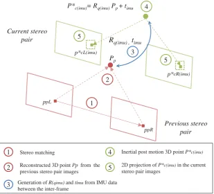
Figure 2 summarizes our idea and highlights five keys steps:

(i)Stereo matching: The detected features are matched between right and left previous images giving a setsp=ppL(j), ppR(j)ofncorrect stereo correspondences (j = 1, ..., m, m the number of points).

(ii) 3D reconstruction: Features from the setsp are reconstructed in 3D using stereo calibration

parameters by triangulation25_{resulting into a setS}

p=P(j)of 3D points representing the position

of the stereo correspondences in the space.

(iii)Inertial motion matrix estimation:IMU information (accelerometer and gyroscope) are acquired and integrated in order to form the inertial inter-frame relative motion composed of R(qimu)

andtimu.

(iv) Calculation of 3D inertial guesses: This inertial motion matrix is then combined withSpin order

to obtain the 3D inertial guesses following the equation of motion (1) described below:

Pimu(j)

Pp

P*c(imu)= Rq(imu)Pp + timu

ppL 2 3 4 5 5 1 2 3 4 1

R_{q(imu) ,}t_imu

Previous stereo pair Current stereo pair 5 ppR Stereo matching

Reconstructed 3D point Pp from the previous stereo pair images

Generation of R(qimu)and timufrom IMU data between the inter-frame

Inertial post motion 3D point P*c(imu)

2D projection of P*c(imu)in the current stereo pair images

p*cL(imu)

p*cR(imu)

Fig. 2. Illustration of the main steps of IMU-assisted feature tracking principle for one point including: stereo matching, 3D reconstruction, IMU motion transformation, and projection into image plane.

The set of 3D post inertial motion features is calledS_c∗=P_c∗_(imu) withPp=[Xp, Yp, Zp]Tand

P_c∗_(imu) =[Xc(imu), Yc(imu), Zci(imu)]T.

(v) Projection into 2D image plane:The components ofS_c∗are projected into the current stereo pair images using the stereo camera parameters as described below:

⎧ ⎪ ⎪ ⎪ ⎪ ⎪ ⎨ ⎪ ⎪ ⎪ ⎪ ⎪ ⎩

p∗_cL(imu) =

u∗_cL(imu) v∗_cL(imu) =

fXc(imu)

Zc(imu) +u0

f Yc(imu)

Zc(imu) +v0

p∗_cR(imu)=

u∗_cR(imu) v_cR∗ _(imu) =

⎡ ⎣f

(Xc(imu)−B)

Zc(imu) +u0

fYC(imu)

Zc(imu) +v0

⎤ ⎦

(2)

where f is the focal length, u0 andv0 are the central pixel’s coordinates, and B the stereo

baseline.

A set s_c∗=p_cL∗ _(imu), p∗_cR(imu) of 2D post inertial motion features is then formed in which a high-confidence tracking area can be built.

3.2. Adaptive local tracking windows

Most of the time, inertial guesses are giving to the KLT a relatively fair estimation of the features to be tracked. That said, and in order to take the full advantage of it, we aim to maximise the use of the KLT by restraining the tracking area to the strict neighbourhood of the inertial guesses. Indeed, restraining the tracking area has two major advantages. First, it reduces the probability of tracking wrong features. Secondly, it increases KLT computational efficiency because of the great reduction in size of the tracking search area. We call these newly defined tracking areas: Adaptive Local Tracking Windows (ALTW) illustrated in Fig. 3.

(1) Let us call s_pc∗ =ppL, ppR; pcL∗ (imu), p∗cR(imu) the set of features regrouping the initial stereo

1

Adaptive Local Tracking Window

2

A(ζ)

3 A(ζ)

4

KLT

KLT Base Local

Tracking window

ws p*cL(imu)

p*cR(imu)

ppL

ppR

A(ζ) IpL

IpR

IcL

IcR

IpL

IpR

IcL

IcR

A(ζ)

A(ζ)

ApL(ζ))

ApR(ζ)) AcL(ζ))

AcR(ζ))

Fig. 3. Illustration of the ALTW concept in four main steps: inertial projection, size calculation of adaptive local tracking windows, sub-set images extraction, and feature tracking with KLT.

(2) Sizes of the adaptive local tracking windows are calculated according to global and local parameters forming the vectorζ:

ζ =|ϕimu| |θimu| |ψimu|d dcr T

(3)

Global parameters [|ϕimu||θimu||ψimu|]Tare the Euler angles resulting from the inertial

inter-image information fromR(qimu). These are influencing all the features in a same manner.

Local parameters [d, dcr]T_{represent, respectively, the disparity and the distance of the feature}

from the image centre. These are specific to each feature relatively to its position in the image. According to the parametersζ, adaptive local tracking window sizeA(ζ) is calculated for each component ofs_pc∗ following the conditions below:

• If the velocityvehicle> 3 m/s and (|ϕimu| or |θimu| or |ψimu|) > 0.009 rads then

A(ζ)=ws+g(|ϕ|,|θ|,|ψ|)+l(d, dcr) (4)

• Otherwise

A(ζ)=ws+l(d, dcr) (5)

wherewsis a constant 9×9 base size of the local tracking window. This initial size can be widen gradually according to the score obtained with the local and global sub-functions, respectively

l(d, dcr)andg(|ϕ|,|θ|,|ψ|). For instance, typical values 0.5◦,1◦, 2◦, 3◦, 4◦ correspond to 7, 9, 16, 27, 41 pixels. The sub-functionsgandlare experimentally expressed as follow:

g(|ϕ|,|θ|,|ψ|)= (1+10×max (|ϕ|,|θ|,|ψ|))

4

Fig. 4. Illustration of adaptive local tracking windows (blue squares). Blue lines—inertial optical flow, red lines—outliers, white lines—inliers.

and

l(d, dcr)=4× d

f ×B +2×

dcr −400

100

(7)

wheref the focal length, andBthe stereo baseline. Notably, a maximum size of 40 square pixels is fixed even if the score ofA(ζ) is found to be higher.

(3) Depending on the local parameters, a maximum of four different ALTW sizes can be obtained. However, we only keep the adaptive local tracking windows with the larger size which is applied to all. Thus, each individual tracking sets_pc∗ has a unique ALTW sizeA(ζ) surrounding each of its components.

(4) For each component ofs_pc∗ , we extract a region of interest, which has the size of the calculated ALTW resulting in a sub-set of four imagesAALTW=ApL(ζ), ApR(ζ);AcL(ζ), AcR(ζ). Figure

4 illustrates use of ALTW on different images.

Before running KLT, a phase correlation stage is done between ApL(ζ) and ApR(ζ) and,

respectively, betweenAcL(ζ) andAcR(ζ).

Phase correlation stage is a fast frequency-based approach giving an estimate of an eventual translational offset between two similar images. If an offset is found, it is then use to refine the position of inertial guesses. Discrete Fourier Transform (DFT) is calculated for the two related ALTW and serves then to compute the cross-power spectrum C as such

C = GaG

−

b

GaG−b

(8)

where

Ga =F

ApL(ζ)

andGb =F{AcL(ζ)} for left pair

Ga =F

ApR(ζ)

andGa =F{AcR(ζ)} for right pair

whereF is the forward DFT and the exponent “−” indicates the conjugate of the DFT andF−1 _is

Then, the cross correlation (8) is converted back to the time domain and the translational shiftυ is deduced from the peak location:

υx, υy

=argmax

(x,y)

F−1{C} (9)

3.3. KLT formulation

The KLT tracker is defined as a non-linear optimisation problem that aims to minimise the squared sum of the intensity differenceebetween two successive imagesIp andIc. This operation is done

over a small patch of size (2wx+1)×(2wy+1) centred, respectively, at the position x=[u, v]T

and the tracking motion modelw(x;p).

e=

wx

−wx

wy

wy

Ip(x)−Ip(w(x; p)

2

(10)

wherewx andwy are two integers usually set to 7,8,10,. . . 21 according to Eq.(9). The local patches

inner pixels are used to create an over constrained system.

The tracking motion model, also calledwarping function w(x;p), is composed of x=[u, v]T _a

pixel coordinate andpa vector of warping parameters.

The KLT starts with an initial value ofp, and iteratively searches for theδpthat aligns the two image patches such that Eq.(10) is minimised. The warping functions can be written following two different models. First, the translational model expressed as

w(x;p)=w(x+b) (11)

The second one is the affine model expressed as:

w(x;p)=w(Ax+b) (12)

where

A=

1+ηxx ηyx

ηxy 1+ηyy

andb=

ηx

ηy

The translational model has the advantage to be fast. However, it is only reliable if the appearance change between subsequent images remains small.p needs to be initialised with a pixel position close enough to its target in order to allow translational-based KLT to cope with large optical flows.

On the other hand, the affine model (or also calledpyramidalKLT) gives more options to deal with spatial deformation of the patches. However, it is computationally more expensive than the translational model. For this implementation, we opted for the translational model (11). In our case, the warping parameterptakes as initial points, an inertial guess:

p=b=

⎧ ⎪ ⎪ ⎪ ⎪ ⎨ ⎪ ⎪ ⎪ ⎪ ⎩

u∗_CL(imu) v_CL∗ _(imu)

for left pair

u∗_CR(imu) v∗_CR(imu)

for right pair

(13)

The latter is re-written with the knowledge of the ALTW (Eqs. (4) and (5), and Fig. 3) as e ⎧ ⎪ ⎪ ⎪ ⎨ ⎪ ⎪ ⎪ ⎩ wx −wx

wy

−wy

ApL(ζ)(x)−AcL(ζ)(w(x+b)) 2

wx

−wx

wy

−wy

Ap R(ζ)(x)−AcR(ζ)(w(x+b))

2 (14)

Instead of searching on the entire image for each correspondence, the KLT only focus on limited areas defined by adaptive local tracking windows calculated earlier (Fig. 3). This presents many advantages:

• First, the inertial projection features hold the full inter-image information (rotation plus translation), which enables the KLT to remain robust to scale changes.

• Secondly, the sub-images only extract the close neighbourhood of the points composing a sets_pc∗ . Consequently, it prevents the KLT from false tracking.

• Thirdly, the computational time of the KLT drops considerably because of the small size of the tracking areas defined by the calculated ALTW.

All these advantages are made possible by the combination of full inertial information combined with 3D geometry and stereoscopy allowing a precise prediction of the tracked features location (see Fig. 2). This is the main difference with related work,13,14_{where inertial features are calculated from}

the rotation matrixRgyroonly using 2D image homography transformation as follows:

⎧ ⎨ ⎩

b=xgyro=Hx

with H =KRgyroK−1

(15)

where H is the 3 × 3 homography matrix andK is the camera calibration matrix. Features are rotated in the image plane according to the gyroscope information and serve as initial conditions to minimize Eq.(10). The warping function of Ryu14follows the translational model and consequently it only requiresb(11) as input for the warping parameter p. On the other hand, Hwangbo13uses a more advanced affine photometric model with eight parametersp=(ηxx, ηxy, ηyx, ηyy, ηx, ηy, α, β),

whereα andβ deal with illumination change. For these two techniques13,14_{based only on rotation}

information scale change remains an issue.

3.4. Inertial dynamic features rejection

The use of full IMU information combined with 3D geometry and stereoscopy brings to each feature a coherent motion behaviour. Additionally, the rigid vehicle-camera-IMU structure jointly moves towards the scene in a unique manner. This gives to the inertial guesses similar projection trend whether if the initial detected were belonging to static or dynamic objects.

Fig. 5. Illustration of the effect of inertial guesses on features belonging to dynamic objects: Top: Consecutive images illustrating a moving truck before (left) and after motion (right); Bottom: Optical flow plotted on the after motion image between detected and: left—tracked feature using Affine KLT; middle—inertial guesses; right—inertial guesses with their respective ALTWs displayed.

4. Motion Estimation

4.1. Local bundle adjustment and trust region method

In this section, the presented solution for motion estimation is a minimalist version of the local bundle adjustment involving only two consecutive stereo pair images. It only focuses on the optimisation of the relative motion parameters between these two views.26Several contributions1,16,18demonstrated that the use of multiple frames bundle adjustment approaches increase the accuracy of VO final position error over long-distance navigation. However, it was also shown that the use of a two frames approach bundle adjustment with a robust features association scheme4,26 _{achieve a position error}

of <1% of the travelled distance while being computationally efficient. This two views scheme fits perfectly our feature tracking strategy, where features over are not tracked over more than two consecutive frames in order to avoid drift in image feature localization.

The non-linear objective functionf to minimise is the image re-projection error function of the motion parameter vectorκexpressed as follows:

min

N

i=1

pcL(i)−f

Pp(i);κ 2

+pcL(i)−f

Pp(i)−B;κ 2

(16)

where

κ =q0 q1 q3 q4 tx ty tz

T

(17)

This motion parameter vectorκ to be optimised is a 1 × 7 vector which consists of the four quaternion elements for the orientation and the translational elements on the three axis (x, y, z).

Non-linear re-projection functionf takes as input,Ppa 3D triangulated feature from the previous

stereo pair and the motion parameterκ(also the baselineBfor right pair features). The link between spatial and planar representations is obtained with the help of the rectified camera matrixKrectin the

way as Eq.(2). The objective is to reduce the pixel distance between the tracked features and their relative re-projected features.

Levenberg–Marquardt (LM) algorithm is widely used to solve bundle adjustment problem.27−28 This technique that was first proposed by Levenberg29and then Marquardt,30is commonly adopted to solve non-linear least square problems because of its easy implementation and its effectiveness. It also belongs to the trust region methods family that guaranties local convergence while avoiding the non-positive definite Hessian problem in contrary to Newton’s method.

κ

Δ

C.P _DL

N DDL Steepest descent

direction

Newton point

C.P:Cauchy Point

DL: Dogleg step

D.DL:Double Dogleg Step Driven by N

N:Intermediate Newton step

Δ:Trust region boundary

Fig. 6. Illustration of dogleg and double dogleg convergence curve.

adjusted along iterations. If the model matches the objective functionf thenis increased, whereas it decreases if the approximation is poor.

4.2. Double dogleg

In this work, instead of using LM algorithm, we decided to adopt DDL trust region method,31which is a variant of the dogleg (DL) algorithm32 to solve the bundle adjustment for motion estimation. It has already been shown that the use of DL trust region technique presents advantages in term of computational cost compared to Levenberg–Marquardt methods for full bundle adjustment applied to 3D structure reconstruction only.33_{DL algorithm is delineated by two lines composed of the steepest}

descent direction and the Newton point direction (see Fig. 6). The optimal trajectory follows the steepest descent direction until reaching the Cauchy point (CP) then converges to the Newton point passing by the DL step.

This later should be intersecting with the trust region boundary. By introducing an intermediate Newton stepN between the CP and the actual Newton point, the behaviour of the DDL algorithm presents a further improvement. Indeed, the optimal curve trajectory crosses the trust region before original DL. This direct control between these two lines (Steepest descent and Newton) by the mean of trust region (characterised by) gives a faster optimisation to the algorithm and is also the main difference with LM algorithm.34

Trust region sub-problem follows a quadratic model(δ) that approximates the objective function f (κ) (16) in such a way that the model is trusted within a limited region k around the current

motion parameter vectorκ:

Qk(δ)=f(κ)+

JTrTδ+1 2δ

T_JT_JT_{δ (18)}

where

r =x−f (κ) andJ = ∂f(κ) ∂κ

Wherer is then×1 residual vector,J is then×7 Jacobian matrix of the functionf(κ) andJTJ is then×napproximation of the Hessian matrix, andIthen×nidentity matrix (nthe number of correspondences).

Solving (18) is not straightforward. In the case where the unconstrained solution δN (Gauss–

δDL=δCP +λ(δCP − δN) forDL

δDDL=δCP +λ(βδCP − δN) forDDL (19)

withβ=0.8γ+0.2 (γ [0,1]) is an adjusting parameter that fixes the position of the intermediate Newton stepN in the Newton direction for the DDL, (see Fig. 6). The minimiser for the Cauchy pointδCP and the Gauss–Newton stepδN are obtained using these equations.

δCP = −

bT_b

bT_Abb δN =A−1b

(20)

where approximated HessianA=JT_{J and the gradientb=J}T_{(x−f(κ)) with the JacobianJ =}

[∂q/∂κ, ∂t/∂κ]T_{andf(κ) is the objective function. Depending on the method chosen (19),λmust}

achieve

δDL= or δDDL= (21)

Thus, in our case the chosen method is DDL, and the current pointκkis updated according to the

constrained trust region as

κk+1= ⎧ ⎨ ⎩

κk−_δCPk ifδCP ≥k

κk+δDDLifδCP kandδNk

κk+δN ifδCP < kandδN ≤k

(22)

After the calculation of the new pointκk+1, the trust regionk+1is then updated according to the

reduction ratioρkbetween the actual residualractand the predicted residualrpreddefined below:

ρk =

ract

rpred

= f (κk)−f (κk+1)

Qk(0)−Qk(δDDL)

(23)

k+1= ⎧ ⎨ ⎩

γ1kifρk< η1

k ifη1≤ρk < η2

γ2kifρk ≥η2

(24)

where 0 <γ1< 1 <γ2and 0 <η1 ≤η2< 1. The value ofkis increased or decreased according to the

quality of the model approximation of the objective functionf (16). The algorithm converges when ||b||≤.

Algorithm 1RANSAC-based motion estimation routine

Input:s

Output:κfinal, sinliers Set:τ =5;

# start of RANSAC routine for motion estimation fork=0 to 50

Nk =0

form the setsby getting 3 random pairs froms initialiseκk =κ0

# call the chosen optimisation process

κoptim=DoubleDogleg(sRNG, κk,) (Algorithm 2)

if(converged)

# get the inliers correspondences for eachpair fromsdo

if(||pcL−pcL∗ ||+||pcR−p∗cR|| <τ)

Nk =Nk+1

endfor

if(Nk>Nbest).

#create an feature the set sinliersf romtheNk

inliers

Nbest=Nk

κbest=κoptim endif

endif endfor

# refinement stage usingκbestsinliers

κfinal=DoubleDogleg(sinliers, κbest) (Algorithm 2) Algorithm 2Double Dogleg minimisation process

Input:pcL, pcR,Pp,κ0 Output:κoptim

Set:k =1,β =0.6667,η1 =0.15,η2=0.75,γ1 =0.5,γ2=2,ρ0 =1,χ =1e−4, k=0,

maxiter=50;

# start of optimisation task

while( not converged and notmaxiter)

if(ρk> 0 )

Compute:

A=JT_{J, b=J}T_{r, ||b||, ||κ}

k||, |||x -f(κk, Pp)||

and ||δCP|| (20)

G.N(Gauss–Newton)=false

if( ||b||_∞<χ or ||r|| <χ ) κoptim=κk

converged

endif endif

if(||δCP|| >k)

δDDL= −(k/||δCP|| )*k

else if( not G.N ) ComputeδN (20)

endif

if( ||δN||≤k)

# take Gauss–Newton direction

δDDL=δN

else

ComputeδDDL(19) endif

if( ||δDDL|| <χ ||κk|| )

κoptim=κk

converged

else

Compute: κnew=κk+δDDL

A=JTJ ,b=J(x -f(κnew, Pp))and ρk(23)

if(ρk> 0)

κk =κnew(22)

endif

update trust region boundary(24)

endif endwhile

4.3. Visual motion estimation algorithm

Let us considers =ppL(i), ppR(i);pcL(i), pcR(i)the set holding all the feature correspondences linking

consecutives stereo image pairs (i = 1, ..., n, n is the number of correspondences). The presented motion estimation algorithm is implemented following a RANSAC-based scheme as a part of an efficient inliers selection strategy. At each step, it starts with the selection from the sets of three random pairs of initial features and their corresponding tracked features. These three random pairs form the setsRNG =ppL(j), ppR(j);pcL(j), pcR(j)(j = 1, 2, 3). The motion parameters ofκis initialised

toκ0=[1 0 0 0 0 0 0]Tas it is a sufficient condition for the motion parameters to converge, especially

when the quality of the feature correspondences are good.

Then, the minimisation method (Algorithm 2) is called taking as input the motion parameterκkand

sRNGfrom whichPp(j)is the 3D position of the previous features. In the case where the optimisation

methods led to a converging solution, the resulting estimation ofκkfor the current setsRNGof random

points is assessed for the whole sets. Each feature correspondence from which the re-projection error falls under a fixed thresholdτ is considered as inlier. At the end of the RANSAC routine,κbesttakes

the value of the motion parameter estimationκkgiving the largest amount of inliers. This enables us

to form a new set of filtered feature correspondencessinliers.

A refinement step runs the minimisation method (Algorithm 2) for a last time using only the set of inlierssinliers obtained fromκbest. This gives the final solution κfinal from which the inter-frame

rotationR(q)and translationtare computed. Relative motion estimations are then accumulated along

the platform’s (vehicle’s) route in order to reconstitute the whole travelled trajectory. Algorithm 1 describes the RANSAC-based motion estimation routine. This RANSAC-based motion estimation routine optimises the motion parameterκand at the same time discards all possible outliers that were contained in the sets.

Processing iteratively a small set of three random pairs gives to this routine a great efficiency. Furthermore, it showed an impressive robustness against outliers especially the ones belonging to dynamic objects such as vehicles, pedestrians, trams, etc. Knowing how much the outliers can be misleading, and especially how a wrong estimation of the motion can dramatically affect the whole generated trajectory, it is very valuable to have reliable motion estimation routine.

5. Experiments

In this section, we present the results of our VO algorithm running on an urban environment dataset35

available at https://wiki.qut.edu.au/display/cyphy/UQ+St+Lucia. In this dataset,35_{a car is equipped}

with stereo cameras (Point GreyR _{Flea2) and an IMU-GPS device (XSens}R _{Mti-g) mounted on} its roof. Visual data consist of 1024× 768 stereo images acquired at 30 Hz. IMU data provide calibrated accelerometer and gyroscope information at 100 Hz, and GPS data at 1 Hz. INS data are also provided in this dataset. It will serve as a reference in the VO trajectory comparison tests. In the first instance, feature tracking performance only will be evaluated. Then, we will assess the impact of feature tracking on the quality of the VO generated trajectories. Finally, it is the accuracy of the VO generated trajectories focusing this time only on motion estimation techniques which will be analysed.

5.1. Feature tracking and processing time performances

Table I. List of KLT techniques with their characteristics.

Techniques Abbreviation Model Pyramid level Patch size

KLT (visual only) T Translational 0 21×21

gyro-assisted KLT without adaptive local tracking windows (gyro)

GT Translational 0 21×21

IMU-assisted KLT without adaptive local tracking windows (gyro+accelerometer)

IT Translational 0 21×21

IMU-assisted KLT (gyro+accelerometer) ITA Translational 0 A(α)/2×A(α)/2

gyro-aided KLT (gyro)13 _{GA Affine 3 21×21}

Table II. KLT techniques: tracking performances, processing time, and time ratio (ITA taken as reference) at different frequencies on dataset35_{full sequence.}

ITA T GT IT GA

Tracking performances (%) 10 Hz 92.5 54.5 56.5 88.3 67.5

5 Hz 85.4 32.2 34.2 75.3 59.2

3 Hz 77.3 18.7 19 62 47.8

Processing time (ms) 10 Hz 18 38 40 31 141

5 Hz 17 34 38 31 138

3 Hz 17 33 36 29 128

Time ratio 10 Hz 1 2.2 2.2 1.7 7.8

5 Hz 1 2 2.2 1.8 8.1

3 Hz 1 1.9 2.1 1.7 7.5

In order to highlight the importance of using full IMU information, three variations of our IMU-assisted KLT method have been tested. Table I describes abbreviations and characteristics of the compared KLT-based techniques.

• The first variation uses accelerometer and gyroscope information and adaptive local tracking windows.

• The second variation is the same as the first one but without adaptive local tracking windows.

• The third variation is the same as the second one but using gyroscope information only.

Results of our IMU-assisted KLT feature tracking in its three variation forms are compared to conventional KLT but also to the Hwangbo’s gyro-aided KLT method.13 In order to have a complete and fair comparison, we adapted their code (https://www.cs.cmu.edu/ myung/IMU KLT/ index.html#source) to our stereo motion scenario, as it is originally designed for monocular camera systems. The evaluation criteria are the rate of inliers over tracked features and KLT processing time. Table II presents feature tracking and time-related performances at different sequence frequencies for the techniques mentioned in Table I.

For the full sequence, a general drop of the percentage of correct tracked features can be observed when the gap between consecutive frames gets bigger (i.e., lower frequency). Besides, a decrease of the processing time decrease can be noticed. This is a logical consequence of the lower number of initial features to track at lower frequency. T loses almost 50% of features on average at 10 Hz and can only save around 20% at 3 Hz. These results are not surprising at all according to the nature of KLT, which hardly copes with scaling. GT which adds gyroscope information slightly improves the performance but remains very similar to T. When using the full IMU information (IT), the tracking performance is greatly improved compared to T and computation time gets also reduced because of the higher precision of the inertial features. Because of the affine approach GA gives better results than GT. This is even truer at low frequency. However, it remains clearly below IT. Additionally, homography-based affine model requires a much higher computation cost. Finally, ITA offers the best tracking performance with the lowest processing time.

0 20 40 60 80 100 1 t 0 t ITA

10Hz 5Hz 3Hz

0 20 40 60 80 100 1 t 0 t IT

10Hz 5Hz 3Hz

0 20 40 60 80 100 1 t 0 t GA

10Hz 5Hz 3Hz

0 20 40 60 80 100 1 t 0 t T

10Hz 5Hz 3Hz

%

% %

%

Fig. 7. Illustration of the full sequence average tracking performance drop for the different techniques as a function of the scale change (GT not displayed here as it is very similar to T).

slope of the different techniques regarding tracking performances against increasing scale change. Indeed, with 77.3% of correctly tracked features even at 3 Hz, ITA is the most robust against scale change compared to his other technique.

Table III presents results of the tracking performance for the different KLT-based techniques in three challenging areas. These happen within the full sequence where the vehicle undergoes obstacles resulting in severe rotations (pitch and roll). In these three cases the results achieved reinforce the findings in Table II.

Performance of T drops completely even at 10 Hz. On the other hand, we note that gyro-based solutions (GT and GA) are giving better performances here than on the full sequence especially at higher frequencies (10 Hz and 5 Hz). This is not the case at 3 Hz where the scale change is too severe between subsequent images. GA gives relatively close results to IT, although it is less valid at 3 Hz. ITA remains far better than the other techniques, coping impressively well with the huge scaling and rotational changes. Comparing performances between ITA and IT confirms the contribution of adaptive local tracking window in the improvement of the tracking performance.

Figures 8, 9, and 10 illustrate two images on the three cited challenging points for each KLT-based technique at 5 Hz. Most of the tracked features from GA belong to far objects. These are also the one that are less affected with scaling. Hence, they are easily mapped by homography. However, in Figs. 9 and 10, GA is severely affected by the large scaling and cannot track any features.

Conversely, ITA and to a less extent IT are able to track features close to the camera presenting large optical flows that can reach more than 100 pixels in translation. These features are really important for motion estimation as they present a significant disparity, which means that they are less subject to errors.

5.2. Impact of feature tracking in motion estimation

Table III. KLT techniques: tracking performances, processing time, and ratio at different frequencies (for three challenging areas) on dataset35_.

Tracking performances (%) ITA T GT IT GA

Bump in a roundabout 10 Hz 97.2 16.3 62.1 89.5 81

5 Hz 89.9 11.6 28 63.5 78.9

3 Hz 79.2 11.6 25.1 49 33.9

1st Humped crossing 10 Hz 95.9 21.3 57.2 89.6 66.3

5 Hz 86.9 11 24.3 63.7 61.2

3 Hz 88.1 18.2 17.7 51.1 46.9

2nd Humped crossing 10 Hz 96.9 13.6 60.4 87.7 87

5 Hz 88 14.8 26.5 76.4 63.5

3 Hz 91.4 13.2 18.1 69.1 34.9

Fig. 11. Trajectories generated with KLT Techniques combined with double dogleg optimization method at 10 Hz, circle represent the end of each trajectory: green ITA; blue IT; cyan GT; yellow T; red GA; black F ground truth reference for final position (defined in Section 5.3 and Fig. 12).

First, T, GT, and GA have a lower rate of tracked features compared to ITA and IT (see Section 5.1). Furthermore, the majority of these features belong to far objects which are in fact coarse and very inaccurate data. Thus, estimation of the motion gives an under estimated travelled distance when it does not fail. Errors accumulation logically leads to large drifts (Fig. 11).

5.3. Motion estimation performances

This sub-section shows the performance of motion estimation regardless of the feature tracking method. The optimisation methods for motion estimation consist of DDL, DL, and SBA implementation of LM.36ITA algorithm will be used for those three methods as the feature tracking technique. Additionally, a filtered INS/GPS trajectory is included in the comparison test. Notably, we found after having aligned INS/GPS trajectory on a satellite image map, it slightly deviates from the road path.

Thus, we defined an as accurate as possible final ground truth position F according to the satellite map and the final images in the dataset35 as illustrated in Fig. 13. Figure 12 shows the trajectories generated with the three techniques at 10 Hz. The trajectory generated using DDL is the one that remains the closest to the INS/GPS. The trajectories generated using DL and LM start slightly drifting from INS/GPS trajectory approximately at half way. However, the drift is not penalising much their respective final positions.

Table IV. Final relative 2D position error against final position F for the different optimization methods using ITA at each frequency on dataset35_{full sequence.}

Double Dogleg Levenberg–

INS/GPS dogleg (ITA) (ITA) Marquardt (ITA)

10 Hz 2D RMS (m) 9.78 m 5.03 m 10.33 m 11.74 m

2D RMS (%) 1.99 % 1.02 % 2.10 % 2.39 %

5 Hz 2D RMS (m) 9.78 m 24.93 m 32.01 m 55.35 m

2D RMS (%) 1.99 % 5.07 % 6.52 % 11.27 %

3 Hz 2D RMS (m) 9.78 m 36.96 m 44.01 m 146.5 m

2D RMS (%) 1.99 % 7.53 % 8.98 % 29.85 %

Fig. 12. Trajectories generated with ITA combined with different optimization methods at 10 Hz: blue INS/ INS/GPS; green DDL; cyan DL; yellow LM; black circle final position F. Left full map/right zoom on the final position.

Fig. 13. Left—Zoom on the final position (white dot) in front of the “Head Hump” road marking highlighted with the red dashed line; Right—Related image from the dataset of the vehicle final position in front of the “Head Hump” road marking highlighted with the red dashed line.

When the image sequence frequency gets lower, motion estimation accuracy logically decreases for all the techniques. However, trajectories generated using DDL, and DL using ITA remains under 10% error of the travelled distance. This demonstrates the robustness of our technique to severe scaling in feature tracking but also in the motion estimation. Table V confirms that DDL is the technique that requires the least iterations to converge to a solution. In Fig. 12 and Table IV, we demonstrated that INS/GPS can be challenged by our method in terms of accuracy in a certain context.

To complement this study and also to show the robustness of our method, we tested our algorithm on KITTI Vision Benshmark37_{raw data sequences (http://www.cvlibs.net/datasets/kitti/raw data.php).}

This dataset consists of 1242×375 rectified stereo images as well as synchronised GPS and IMU data (accelerometer and gyroscope) acquired at 10 Hz. Contrary to the first dataset35 _{the IMU are}

Table V. Average number of iterations for all frequencies on dataset35_{full sequence with the different}

optimisation methods.

Double dogleg (ITA) Dogleg (ITA) Levenberg–Marquardt (ITA)

Iterations 7.1 9.8 12.6

Table VI. Final relative 2D and 3D position error for ITA using double dogleg and LiViso2 methods on KITTI vision Benchmark raw data sequences (http://www.cvlibs.net/datasets/kitti/raw data.php) and on dataset35_.

ITA with DDL LibViso238

Distance # of 2D 3D 2D 3D

(m) Frames RMS % RMS % RMS % RMS %

KITTI 2011 09 26 0001 106.75 108 0.50 0.53 0.95 0.96

2011 09 26 0002 80.64 77 0.34 0.34 1.40 1.47

2011 09 26 0005 69.10 154 6.28 6.28 7.37 7.38

2011 09 26 0009 333.36 447 2.71 2.71 1.42 1.43

2011 09 26 0014 164.2 314 1.62 1.99 2.34 2.54

2011 09 26 0027 344.64 188 0.82 0.82 1.47 1.47

2011 09 26 0051 253.08 438 0.24 0.26 0.92 0.94

2011 09 26 0084 238.96 383 0.36 0.37 1.01 1.08

2011 09 26 0091 198.09 340 0.20 0.24 0.52 0.54

2011 09 260.5018 0117 323.14 660 2.57 2.59 2.04 2.06

QUT35 _{10 Hz 501.42 600 1.02 – 12.36 –}

the integration of these measurements over the time. It is especially true for the accelerations. This, results into inaccurate inertial angular/position data at the available sampling rate. For this reason, the use of our algorithm using double dogleg with ITA could be only run at 10 Hz and could not be re-sampled at lower frequency as for dataset.35

Table VI shows the results on 10 sequences from KITTI Vision Benshmark37_{of our algorithm and}

libViso2 method (http://www.cvlibs.net/datasets/kitti/raw data.php) against the provided GPS taken as reference here.

On overall our algorithm and LibViso238_{method give accurate results achieving a position error}

of <1% of the travelled distance on certain cases, and without exceeding 3% position error of the travelled distance (expect for sequence 2011 09 26 0005, but GPS reference might be biased).

Except for the sequences 2011 09 26 0009 and 2011 09 26 00117 in KITTI Vision Benshmark37 raw data sequences (http://www.cvlibs.net/datasets/kitti/raw data.php), our algorithm is more accurate than LibViso238method.

However, LibViso238 showed more difficulty on dataset35 to keep the same accuracy than for KITTI Vision Benshmark raw data sequences (http://www.cvlibs.net/datasets/kitti/raw data.php). As mentioned in Sections 5.1 and 5.2, this ability of ITA to keep tracking features close to the camera presenting large optical flows make a real difference comparing to LibViso238_{on dataset.}35

Therefore, we demonstrated that with an efficient and clever association between inertial data and visual information we are able to enhance feature tracking of the conventional KLT.

This solution is also independent from external sources of information (e.g., satellites) and can thus be employed as an interesting alternative to GPS or INS/GPS. Additionally, by offering the ability to process low frame rate sequences while keeping good performance and low computation meaning that the IMU-assisted KLT can be easily implemented for real-time applications.

6. Conclusion and Future Work

data. This significantly narrows the matching search region and consequently reduces ambiguity. Resulting adaptive local tracking windows enable us to precisely bounder areas of the inertial predictive features. This gives the ability to the IMU-assisted KLT to maintain a high tracking rate and to remain robust against scaling by handling very large motions while keeping a low computational cost. This also guarantees accurate tracking of close features which are better quality. Results obtained with the proposed feature tracker demonstrate higher performance than aided affine model, gyro-only translational model. Even in the worst cases of severe scale change, the rate of successful tracks does not go below 80% while the feature tracking performance of other techniques clearly collapse. It has been shown that tracked features with the IMU-assisted KLT enhances the estimated visual-based motion. Additionally, double dogleg optimisation technique was adopted in the motion estimation scheme. Its association to our IMU-assisted KLT method offers a better alternative than LM and GN on different datasets. VO performances lie below or around 1% error of the travelled distance and it also demonstrates higher accuracy than INS/GPS in certain conditions. Future work, aims to develop an embedded navigation technology based on this research including a small IMU-stereo camera set up capable of reproducing same accurate results.

Acknowledgements

The research leading to these results has received funding from Thales and E.S.A (European Space Agency). We would like to thank them for their help and support.

References

1. D. Nister, O. Naroditsky and J. Bergen, “Visual Odometry,” Proceedings of the IEEE Conference on Computer Vision and Pattern Recognition, Washington, D.C., USA, vol. 1, (Jun. 2004) pp. 652–659. 2. M. Boulekchour, N. Aouf and M. Richardson, “Robust L∞convex pose-graph optimisation for monocular

localisation solution for unmanned aerial vehicles,”Proceedings of the Institution of Mechanical Engineers, Part G: Journal of Aerospace Engineering, 229(10), 1903–1918 (2014).

3. T. Mouats, N. Aouf, L. Chermak and M. Richardson, “Thermal stereo odometry for UAVs,”IEEE Sensors J.15(11), 6335–6347 (2015).

4. A. Howard, “Real-Time Stereo Visual Odometry for Autonomous Ground Vehicles,”Proceedings of the IEEE International Conference on Intelligent Robots and Systems, Nice, France (Sep. 2008) pp. 3946–3952. 5. N. S¨underhauf, P. Protzel, “Stereo odometry — a review of approaches”, Chemnitz University of Technology

Technical Report, March, 2007.

6. B. D. Lucas and T. Kanade, “An Iterative Image Registration Technique with an Application to Stereo Vision,”Proceedings of the 7th International Joint Conference on Artificial Intelligence,Vancouver, B.C., Canada, vol. 2, (1981) pp. 674–679.

7. J. Shi and C. Tomasi, “Good Features to Track,”Proceedings of the IEEE Conference on Computer Vision and Pattern Recognition, Seattle, W.A., USA, (Jun. 1994) pp. 593–600.

8. S. Baker and I. Matthews, “Lucas-kanade 20 years on: A unifying framework,”Int. J. Comput. Vis.56(3), 221–255 (2004).

9. J.-Y. Bouguet, “Pyramidal Implementation of the Affine Lucas Kanade Feature Tracker Description of the Algorithm,”OpenCV documentation, Intel Corporation, Microprocessor Research Labs, (1999).

10. T. Zinßer, C. Gr¨aßl and H. Niemann, “Efficient feature tracking for long video sequences,”In:Joint Pattern Recognition Symposium, (Springer Berlin Heidelberg, 2004) pp. 326–333.

11. S. N. Sinha, J.-M. Frahm, M. Pollefeys and Y. Genc, “Feature tracking and matching in video using programmable graphics hardware,”Mach. Vis. Appl.22(1), 207–217 (2007).

12. H.-K. Lee, K.-W. Choi, D. Kong, and J. Won, “Improved Kanade-Lucas-Tomasi Tracker for Images with Scale Changes,” Proceedings of the IEEE International Conference on Consumer Electronics, Berlin, Germany, (Sep. 2013) pp. 33–34.

13. M. Hwangbo, J.-S. Kim and T. Kanade, “Gyro-aided feature tracking for a moving camera: Fusion, auto-calibration and GPU implementation,”Int. J. Robot. Res.30(14), 1755–1774 (2011).

14. Y.-G. Ryu, H.-C. Roh and M.-Y. Chung, “Video Stabilization for Robot Eye Using IMU-Aided Feature Tracker,”Proceedings of the IEEE International Conference on Control Automation and Systems, Gyeonggi-do, Korea, (Oct. 2010) pp. 1875–1878.

15. S. Tanathong and I. Lee, “Translation-based KLT tracker under severe camera rotation using GPS/INS data,”IEEE Geoscience Remote Sensing Lett.11(1), 64–68 (2013).

16. D. Scaramuzza and F. Fraundorfer, “Visual odometry [tutorial],”IEEE Robot. Autom. Mag.18(4), pp. 80–92 (2011).

18. K. Konolige, M. Agrawal and J. Sola, “Large-Scale Visual Odometry for Rough Terrain,”In:Robotics Research, (Springer Berlin Heidelberg, 2011) pp. 201–212.

19. J.-P. Tardif, M. George, M. Laverne, A. Kelly and A. Stentz, “A New Approach to Vision-Aided Inertial Navigation,”Proceedings of the IEEE/RSJ International Conference on Intelligent Robots and Systems, Taipei, Taiwan, (Oct. 2010) pp. 4161–4168.

20. A. B. Chatfield,Fundamentals of High Accuracy Inertial Navigation, Reston, V.A., USA, vol. 174. (AIAA, Sep. 1997).

21. A. Makadia and K. Daniilidis, “Correspondenceless Ego-Motion Estimation Using an IMU,” inProceedings of the IEEE International Conference on Robotics and Automation, (2005) pp. 3534–3539.

22. F. M. Mirzaei and S. I. Roumeliotis, “A Kalman filter-based algorithm for IMU-camera calibration: Observability analysis and performance evaluation,”IEEE Trans. Robot.24(5), pp. 1143–1156 (2008). 23. A. Martinelli, “Vision and IMU data fusion: Closed-form solutions for attitude, speed, absolute scale, and

bias determination,”IEEE Trans. Robot.28(1), pp. 44–60 (2012).

24. S. Leutenegger, S. Lynen, M. Bosse, R. Siegwart and P. Furgale, “Keyframe-based visual–inertial odometry using nonlinear optimization,”Int. J. Robot. Res.34(3), pp. 314–334 (2015).

25. R. I. Hartley and P. Sturm, “Triangulation,”Comput. Vis. Image Understanding68(2), pp. 146–157 (1997). 26. A. Geiger, J. Ziegler and C. Stiller, “Stereoscan: Dense 3d Reconstruction in Real-Time,”Proceedings of

the IEEE Symposium on Intelligent Vehicles, Baden-Baden, Germany, (Jun. 2011) pp. 963–968.

27. N. S¨underhauf, K. Konolige, S. Lacroix and P. Protzel, “Visual Odometry using Sparse Bundle Adjustment on an Autonomous Outdoor Vehicle,”In:Autonome Mobile Systeme, (Springer Berlin Heidelberg, 2006) pp. 157–163.

28. C. Wu, S. Agarwal, B. Curless and S. M. Seitz, “Multicore Bundle Adjustment,”Proceedings of the IEEE Conference on Computer Vision and Pattern Recognition, Providence, R.I., USA (2011) pp. 3057–3064. 29. K. Levenberg, “A method for the solution of certain problems in least squares,”Quarterly Appl. Math.2,

164–168 (1944).

30. D. W. Marquardt, “An algorithm for least-squares estimation of nonlinear parameters,”J. Soc. Ind. Appl. Math.11(2), pp. 431–441 (1963).

31. J. E. Dennis, Jr and H. H. W. Mei, “Two new unconstrained optimization algorithms which use function and gradient values,”J. Optimization Theory Appl.28(4), pp. 453–482 (1979).

32. M.J. Powell, “A new algorithm for unconstrained optimization”, Nonlinear programming,Proceedings of a Symposium Conducted by the Mathematics Research Center, the University of Wisconsin–Madison, (May 1970) pp. 31–65

33. M. L. A. Lourakis and A. A. Argyros, “Is Levenberg-Marquardt the Most Efficient Optimization Algorithm for Implementing Bundle Adjustment?,”Proceedings of the IEEE International Conference on Computer Vision, Beijing, China, vol. 2, (Oct. 2005) pp. 1526–1531.

34. W. Sun and Y.-X. Yuan,Optimization Theory and Methods: Nonlinear Programming, vol. 1. (Springer Berlin Heidelberg, 2006).

35. M. Warren, D. McKinnon, H. He and B. Upcroft, “Unaided Stereo Vision Based Pose Estimation,”

Proceedings of the Australasian Conference on Robotics and Automation, Brisbane, Australia, (Dec. 2010). 36. M. I. Lourakis and A. A. Argyros, “SBA: A software package for generic sparse bundle adjustment,”ACM

Trans. Math. Software36(1), pp. 1–30 (2009).

37. A. Geiger, P. Lenz, C. Stiller and R. Urtasun, “Vision meets robotics: The KITTI dataset,”Int. J. Robot. Res.(2013).