QQ plot for assessment of Gaussian Process wind turbine power curve error distribution function

9th European Workshop on Structural Health Monitoring July 10-13, 2018, Manchester, United Kingdom

QQ plot for assessment of Gaussian Process wind turbine power curve

error distribution function

Ravi Kumar Pandit, David Infield

University of Strathclyde, United Kingdom, E-mail ravi.pandit@strath.ac.uk/david.infield@strath.ac.uk

Abstract

Performance monitoring based on available SCADA data is a cost effective approach for condition monitoring of a wind turbine. Performance is conventionally assessed in terms of the wind turbine power curve that represents the relationship between the generated power and hub height wind speed. Power curves also play a vital role in energy assessment, and performance and warranty formulations. It is considered a most important curve for analyzing turbine performance and also helps in fault detection. Conventional power curves as defined in the IEC Standard take considerable time to establish and are far too slow to be used directly for condition monitoring purposes. To help deal with this issue the Gaussian process (GP) concept is introduced.

A Gaussian process (GP) is a nonlinear machine learning technique useful in interpolation, forecasting and prediction. The accuracy of fault identification based on a GP model, depends on its error distribution function. A QQ plot is a useful tool to analyze how well given data follows a specific distribution function.

The objective of this paper is to apply QQ plots in the assessment of the error distribution function for a GP model. The paper will outline the advantages and limitations of the QQ plot approach.

Keywords: Condition monitoring, Gaussian Process, power curve, probability distributions functions

1. Introduction

The uncertainty and variability of wind creates operational challenges and affects the efficiency of the wind turbine. In order to overcome such problems, advanced wind power forecasting based algorithms are used. Forecasting helps to reduce the uncertainty associated with variable renewable generation and helps to accommodate the changes of wind more efficiently via commitment or de-commitment of conventional generators [1]. It also reduces the cost of balancing the overall system; thus wind power estimation is important for energy reserve scheduling, and it is also useful in condition monitoring [2,3].

neighbor clustering (kNN), fuzzy c-mean clustering and machine learning processes, such as Gaussian Processes, are now finding application for non-parametric approaches to engineering problems, as summarized in [5,6]. Because of the intrinsic nonstationary nature of wind, models such as ANN, fuzzy logic or kNN are limited to very short-term estimation (1-4 hours ahead), with rather inaccurate results for longer term prediction [7]. However, in case of a GP this effect is not so pronounced. GP is a non-parametric machine learning approach that relies in very few assumptions for model construction. It can work efficiently with reasonable SCADA datasets and has considerable potential for condition monitoring. Confidence interval comes with GP fitting model which is quite useful in analyzing the uncertainty associated with turbine as suggested in [8] As in [9], it is clearly demonstrated a GP based model for power forecasting provides 4% to 11% improvement in forecasting accuracy over an artificial neural network model. The network integration cost associated with wind power is significant but can be substantially reduced by forecasting and effective GP application to this is clearly demonstrated in [10].

In a multivariate model like a Gaussian Process, the probability distribution (pdf) function of model errors can be useful in performance monitoring. In a statistical model, identification of the correct distribution function is key to its performance. For example, confidence intervals are very critical for GP model evaluation or identifying the faults in the wind turbines and these confidence intervals directly depend on the assumption of normality, so model performance is very sensitive to departures from normality. Hence, accurate assessment of distribution function plays a vital role in condition monitoring using a GP.

The quantile-quantile plot (Q-Q plot) is an effective graphical tool for analyzing distribution functions. A QQ plot can be used to compare samples to each other or one sample with a theoretical distribution (e.g. normal). Analysis can reveal valuable information, for example differences in location, spread and shape of datasets [11]. Whether data is accurately represented by normal or Gaussian distribution function depends on the correlation between the test data and the normal quantiles measurements. The QQ plot should be approximately a straight line for normal data for a high positive correlation. Moreover, any outliers in the data are easily identified in the QQ plot. Dhar et al in [12], used a QQ plot for multivariate analysis based on spatial quantiles and described the multivariate QQ plot and their asymptotic properties. This information gives a clearer picture of the operational characteristics of a wind turbine as compared to other available tools like density plots or histograms. The use of QQ plots to compare two samples of data can be viewed as a non-parametric approach to comparing their underlying distributions which makes them an ideal choice for GP power curve distribution analysis. The objectives of this paper are to introduce the concept of the Gaussian Process to power curve fitting and to present QQ plots for predicted GP power curves for different months of data in order to assess how well the results conform to the assumed Gaussian error distribution.

2. Power curve and its data preprocessing

nonlinear relationship between hub wind speed and capture power of a wind turbine can be expressed by equation (1),

(1)

where, P = power output (W); = air density (kg/ ); = wind speed (m/ ) ; A = swept area ( ) = aerodynamic efficiency of a wind turbine.

From equation (1), it is found that capture power is directly proportional to the air density. Air density changes with turbine site and altitude and specially with ambient temperature hence air density correction needs to be applied as per IEC Standard 61400-12-1, [14] using equation (2),

(2)

where and are the corrected and measured wind speed respectively and the ambient air density, can be derive by equation (3),

(3) where T is temperature in Kelvin and B is the barometric pressure in mbar.

The available SCADA comes with measurement errors which ultimately affects investigation or analysis. In short, it affects the accuracy of any models used. Hence it is necessary to clean SCADA data to remove as far as possible erroneous or misleading data. In order to remove such errors, filtration criterion being used cover timestamp mismatch, power with negative values, curtailment etc. After judging the measured power curves (figure 1,3 and 5) on such filtration criterion, measurement errors are reduced and closely matching with ideal power curves as shown in figure 2,4 and 6.

Figure 1: measured power curve for Jan,2012 Figure 2: filtered power curve for Jan,2012

Figure 5: measured power curve for Oct,2012 Figure 6: filtered power curve for Oct,2012

3. Power curve modeling using Gaussian Process (GP)

A Gaussian Process (GP) is a Bayesian, non-parametric, non-linear regression machine learning approach widely used in probabilistic regression problems, for example, [15,16]. Because of its flexibility, basis in probability theory and ease of modelling (it requires very few assumptions) it is an ideal approach for many forecasting and prediction related issues. A GP mathematically defined by its mean and covariance functions (or kernel) as given in equation (4),

(4)

where, is the mean function, ∑ is the covariance function that has an associated probability density function:

= (5)

where is defined as determinant of , is the dimension of random input vector , and µ is mean vector of . The term under exponential i.e. is an example of a quadratic form. A covariance function describes the dependency of two variables with respect to each other and is the heart of any GP model; it signifies the similarity between two points and hence determines closeness between two points. There are various available covariance functions described in [16] and selection is based on nature of the data. The squared exponential covariance function is commonly applied and will be used in this paper. For any finite collection of inputs , It is defined as:

(6) SCADA data of the wind turbine comes with sensor errors so it is desirable to add a noise term to the covariance function in order to improve the accuracy of the GP model. Hence equation (6) modified to be:

(7) where and are known as the hyper-parameters. Signifies the signal variance and

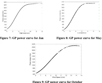
Gaussian Process theory as describe above, has been applied to processed power curve data (figures 2,4 and 6) and the estimated power curve based on the GP model is shown in figures 7, 8 and 9.

Figure 7: GP power curve for Jan Figure 8: GP power curve for May

Figure 9: GP power curve for October

Due to the non-parametric behavior of GP, residual analysis became vital in order to examine the nature of distribution function. Mathematically, residuals are the difference between measured and estimated values and can be expresses as,

(8)

where r is the residual, the measured value and the estimated values predicted by the model.

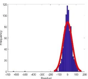
The time series residual plots for January, May and October months predicted GP power curve are shown in figure 10 ,12 and 14 and their frequency distribution of the residuals are shown in figure 11,13 and 15 together with fitted Gaussian distribution and it shows that the residuals are close to being Gaussian however there is no such indication which one of them are more Gaussian.

Figure 12: Residual plot for May,2012 Figure 13: Histogram distribution fit for May,2012

Figure 14: Residual plot for Oct,2012 Figure 15: Histogram distribution fit for Oct,2012

These distribution functions will be assessed using QQ plots in next section.

4. Theoretical Background of quantile– quantile (QQ) plot

The quantile–quantile or Q–Q plot is a simple graphical method used to compare collections of data, or theoretical distributions and help in distribution function identification. In our case it will be used to identify any deviation from normality of errors assumed in GP modelling, specifically it will provide useful information on whether the distribution function is skewed or light tailed. In a Q–Q plot, sample of datasets starting from small to large values are taken and then plotted against the expected value for the specified distribution (i.e. Normal distribution in our case) at each quantile in the sample datasets, [17]. A theoretical Q–Q plot examines whether or not a sample ….., has come from a distribution with a given distribution function . The plot displays the sample of quantiles ,…… against the distribution

quantiles , where . The selection of quantiles in Q–Q

plot purely based on the number of values in the sample datasets. For example, if sample datasets contains then the plot uses quantiles.

of the specified distribution at the same quantiles being described. If the resulting QQ plot is linear then it signifies that the two sets of sample datasets are likely come from same distribution function.

In order to measure the asymmetry of the distribution function its mean, skewness is calculated. Basically, skewness is able to tell the extent to which the model distribution differs from the Gaussian distribution hence depth analysis of skewness can provide useful information. Jean Dickinson, [17], suggests that a QQ plot easier to use than comparing histogram plots in order to judge skewness or more accurately assess whether the distribution tails are thicker or thinner than a normal distribution. In addition to that, a QQ plot is also useful in providing information about such graphical properties as shape, location, size, and skewness are similar or different for two distributions. Another advantage of the QQ plot well describe by M. B. Wilk, [18], is that there no need to defined underlying parameters since it usually taken to be the standard distribution in a group of distributions unlike P-P (probability versus probability) plot which requires specification of the underlying parameters. In addition to that the P-P is plot is more sensitive to the differences in the middle part of two distributions whereas QQ plot is more sensitive to the differences in the tails of the two distributions.

The use of Q–Q plots to compare two samples of data can be viewed as a non-parametric approach to comparing their underlying distributions which makes ideal choice for GP power curve distribution analysis. As described in previous section, for GP models the residuals should be Gaussian distributed. An ideal QQ plot would be a straight line with unity gradient signify the predicted distribution function perfectly fits theoretical distribution.

Figure 16: GP QQ plot, Jan,2012 Figure 17: GP QQ plot, May,2012

QQ plots have been calculated for predicted GP power curves for different months of data. QQ plots have been calculated for all three different months (as shown in figures 16,17 and 18) and assessed in terms of RMSE (Root mean square error), MAE (mean absolute error) and MSE (mean square error) in next section. If we compare the histograms with the QQ plots for the different months, then there is clear difference in terms of judging the distribution function. For example, in the case of January, the histogram shows a smooth fitting while the QQ plot for same month shows that the tails are not fitted correctly. Similarly, conclusions apply to May and October. In short, the histogram not easily able to present information about on what is happening in the tails of the distribution function while this information is clearly captured in the QQ plots as shown in figure 18,17 and 18. So in order to get better resolution on tails, use of QQ plot is preferable. The QQ plot can suggest further investigation on parameters like skewness and kurtosis for judging the accuracy of Gaussian distribution function. Histogram plots based on binning method have disadvantages compared to QQ plots which is explained in [19,20,21] and summarized as follows:

1. The binning suppresses the nature and details of the error distribution which are more often significant for condition monitoring purposes. For example, binning does not give an accurate view of what’s going on in the tails, and also often on in the central section.

2. In order to develop an effective binning algorithm, information about bin origin and bin width needs to know since this ultimately affects the appearance of the histogram.

3. Comparisons between two histograms are more problematic than that of judging the fit of a group of points to a straight line.

The difference between the measured and estimated values can be defined by mean absolute error (MAE):

(9) In terms of residuals, (10)

In order to assesses the quality of an estimator or predictor, mean squared error (MSE), [22], is widely used for measuring of how close a fitted line is to the data points. In

terms of mathematically expression, MSE is defined as,

(11)

Similarly, in terms of residuals, (12)

To quantify the magnitude of the residuals (i.e. the difference between observed and modelled values, root mean square error (RMSE) is commonly used; defined as, [23]:

(13)

where are the GP predicted values for different predictions, and are the measured values. In terms of residuals this is:

(14)

presence of larger number of data point in January as compared to the other months and hence distribution function in QQ plot is smooth and closely fitted as evidences by numerically calculated values of RMSE, MAE and MSE given in Table 1 below.

Month RMSE MAE MSE

Januray,2012 0.66539 0.46479 0.44275

May,2012 1.902 1.031 3.6177

October,2012 3.1271 1.5087 9.779

Table 1: RMSE, MAE and MSE calculated values for different months of datasets

5. Conclusion and future work

Predicted power curves developed using GP models for different seasonal SCADA datasets have been calculated. QQ plots of residuals of the GP power curves have been used to describe distribution functions. Residual QQ plots of predicted GP power curve indicates the distribution is well matched to the Gaussian distribution in case of the January dataset and calculated values of RMSE, MSE and MAE reflect this. The RMSE, MSE and MAE value of residual QQ plot describes the goodness of fit of the predicted distribution function and these were evaluated for the available SCADA data. This assessment of the distribution function is difficult to make simply using histograms due to the use of binning method as explained section 4. Important parameters such as distribution skewness and the tails are important for identifying potential wind turbine faults using GP and these are difficult to assess using histograms alone. It has been demonstrated that QQ plots can be very effective.

The future work is to use the methods developed for anomaly analysis and detection for wind turbine condition monitoring.

Acknowledgements

This project has received funding from the European Union’s Horizon 2020 research and innovation programme under the Marie Sklodowska-Curie grant agreement No 642108.

References

1. L. Bird, M. Milligan, and D. Lew National Renewable Energy Laboratory,

“Integrating Variable Renewable Energy: Challenges and Solutions, ”

2. A. Costa, A. Crespo, J. Navarro, G. Lizcano, H. Madsen, and E. Feitosa, “A review on the young history of the wind power short-term prediction,” Renew. Sustain. Energy Rev., vol. 12, no.6, pp. 1725–1744, 2008. [Online]. Available:

http://www.sciencedirect.com/science/article/pii/S1364032107000354

3. M. Lei, L. Shiyan, J. Chuanwen, L. Hongling, and Z. Yan, “A review on the forecasting of wind speed and generated power,” Renew. Sustain. Energy Rev., vol. 13, no. 4, pp. 915–920, 2009. [Online]. Available:

4. Vaishali Sohoni, S. C. Gupta, and R. K. Nema, “A Critical Review on Wind Turbine Power Curve Modelling Techniques and Their Applications in Wind Based Energy Systems, ” http://dx.doi.org/10.1155/2016/8519785.

5. Lydia M, Immanuel Selvakumar A, Suresh Kumar S, Edwin Prem Kumar G (2013) “Advanced algorithms for wind turbine power curve modeling,” IEEE Trans Sustainable Energy 4 (3):827–835.

6. Delshad Panahi, Sara Deilami, Mohammad A.S. Masoum, “Evaluation of Parametric and Non-Parametric Methods for Power Curve Modelling of Wind Turbines,” 9th International Conference on Electrical and Electronics Engineering (ELECO), doi: 10.1109/ELECO.2015.7394497.

7. M. G. De Giorgi, A. Ficarella, and M. Tarantino, “Error analysis of short term wind power prediction models,” Appl. Energy, vol. 88, no. 4, pp. 1298–1311,

2011. [Online].Available:

http://www.sciencedirect.com/science/article/pii/S030626191000437X.

8. R. K. Pandit and D. Infield, "Using Gaussian process theory for wind turbine power curve analysis with emphasis on the confidence intervals," 2017 6th International Conference on Clean Electrical Power (ICCEP), Santa Margherita Ligure, 2017, pp. 744-749. doi: 10.1109/ICCEP.2017.8004774.

9. Niya Chen, Zheng Qian, “Wind Power Forecasts using Gaussian Processes and Numerical Weather Prediction,” IEEE Transactions on Power Systems ,10.1109/TPWRS.2013.2282366.

10.Joseph Bockhorst, Chris Barbe, “Gaussian Processes for Short-Horizon Wind Power Forecasting,” http://www.cs.uwm.edu/~joebock/papers/maics10.pdf 11.Wilk, M. B. and Gnanadesikan, R. (1968), “Probability Plotting Methods for the

Analysis of Data,” Biometrika, 55, 1-17.

12.Subhara Sankar Dhar, Biman Chakraborty and Probal Chaudhuri, “Comparison of multivariate distributions using quantile–quantile plots and related tests Bernoulli,” 20(3), 2014, 1484–1506. DOI: 10.3150/13-BEJ530.

13. “Modelling of the Variation of Air Density with Altitude through Pressure, Humidity and Temperature,” WindPRO / ENERGY, EMD International A/S 14.Wind Turbines—Part 12-1: Power Performance Measurements of Electricity

Producing Wind Turbines, British Standard, IEC 61400-12-1, 2006.

15.Ping Li, Songcan Chen, “A review on Gaussian Process Latent Variable Models, CAAI Transactions on Intelligence Technology (2016),”

16.C. E. Rasmussen & C. K. I. Williams, “Gaussian Processes for Machine Learning,” the MIT Press, 2006, ISBN 026218253X.

17.Jean Dickinson Gibbons Subhabrata Chakraborti, “Nonparametric Statistical Inference,” Fourth Edition, Revised and Expanded.

18.M. B. Wilk and R. Gnanadesikan. “Probability Plotting Methods for the Analysis of Data,” Biometrika, Vol. 55, No. 1 (Mar., 1968), pp. 1-17.

http://www.jstor.org/stable/2334448

19.Wilk, M.B. and R. Gnanadesikan. 1968. “Probability plotting methods for the analysis of data,”Biometrika 55: 1-17

20.John A. Rice. “Mathematical Statistics and Data Analysis,”3rd edition

22. Neyman, J. (1937). "Outline of a Theory of Statistical Estimation Based on the Classical Theory of Probability,” Philosophical Transactions of the Royal Society A. 236: 333 380. oi:10.1098/rsta.1937.0005.