Restricted structure predictive control for linear and nonlinear systems

Restricted Structure Predictive Control

For Linear and Nonlinear Systems

M.J. Grimble*/**, Pawel Majecki*

*Industrial Systems and Control Limited, 36 Renfield Street, Glasgow, G2 1LU, Scotland, U.K.,

(e-mail: [email protected])

**Industrial Control Centre, University of Strathclyde, 204 George Street, Glasgow, G1 1XW, Scotland, U.K.

(e-mail: [email protected]).

Abstract: An optimal predictivecontrol algorithm is introduced for the control of

linear and nonlinear discrete-time multivariable systems. The controller is specified in a “restricted structure” form involving a set of given linear

transfer-functions and a set of gains that minimize a Generalized Predictive Control (GPC) cost-index. The set of functions can be chosen as proportional, integral and

derivative terms; however, a wide range of controller structures is possible. This is

referred to as Restricted-Structure GPC control.

The multi-step predictive control cost-function is novel, since it includes

weightings on the “low-order” controller gains and the rate of change of gains.

This considerably improves the numerical computations ensuring critical inverse

computations cannot lead to a singular matrix. It also provides the option of adding

soft or hard constraints on the controller gains which provides additional flexibility

for control design. The ability to include a plant model that can include a general

nonlinear operator is also new for restricted structure control solutions.

The low-order controller provides a potential improvement in robustness, since it

is often less sensitive to plant uncertainties. The simple controller structure also

enables relatively unskilled staff to retune the system using familiar tuning terms,

and provides a potentially simpler QP problem for the constrained case.

Keywords: Nonlinear, restricted structure, predictive, minimum-variance, PID.

1. Introduction

The proposed Restricted Structure (RS) controller is an attempt to obtain the benefits of model based predictive control but using a low-order classical structure that can easily be retuned using familiar tuning terms. If adequate performance can be obtained the low-order controller often provides better robustness and can be implemented with lower computing resources. The PID controller is just one option for the choice of low-order controller structure, where the optimal gains are provided by the optimized solution.

The PID controller is very effective in industry and is used successfully across industrial sectors. However, if systems involve difficult dynamics, such as open-loop unstable or non-minimum phase behaviour, transport-delays, or interactions; then ‘multi-loop’ or ‘decentralized’ PID control can provide poor performance. A higher-order controller may then be required and one that can deal formally with multivariable system dynamics. It is then reasonable to extend the controller structure by including other terms like a time-constant or a double integrator term.

Richalet developed simple approaches to Model Predictive Control (MPC), and introduced the idea of using a functional basis (Richalet et. al. 1978, Richalet et. al. 1993,

Rossiter et. al. 2002, Richalet 1998). The first applications took place in the early 70's, and since that time there have been many applications Khadir and Ringwood (2008). The optimal control approach in the following also requires functions to be defined, but these relate to the structure of the controller to be implemented such as extended PID. The proposed approach is a special form of Generalized Predictive Control (GPC).

controller parameters whereas the current work allows the gains to be time-varying. Moreover, the previous contributions assumed linear system models but in the following, a nonlinear model represented by an unstructured model is included.

The RS multivariable controller is defined here in terms of a set of frequency-sensitive functions, multiplied by gains that are found to minimise an extended GPC cost-function. The method will be referred to as Restricted Structure-Generalized Predictive Control (RS-GPC). In the RS-GPC approach introduced below the functions that determine the RS controller are specified in the frequency-domain. The controller gains are computed to minimize a cost-index, which can penalize deviations in controller gain and the rate of change of these gains. The gains vary to compensate for any changes in the reference or disturbance signals.

There are many differences with traditional MPC theory, which may be listed as follows:

1. The restricted structure controller (within the control loop) is low-order, possibly

half the usual order, which provides opportunities for improved robustness and a

simplified on-line algorithm.

2. It may be used to tune classical controller structures (like auto-tuning).

3. The inclusion of gain and rate of change of gain terms in the criterion enables soft constraints to be applied to the controller parameter or gain-variations.

4. The feedback gains are optimized and not future control trajectories, so that the

constrained version enables constraints on controller gains to be introduced, not

available in standard MPC (the usual MPC constraints may also be included).

1.1 Methods of Computing Low-Order Optimal Controls

A fixed-structure and low-order control scheme for Nano-positioning systems was developed by Eielsen et al. (2013). The authors noted “The control schemes are

fixed-structure, low-order control laws, for which few results exist in the literature with regards

to optimal tuning.” There are powerful optimization algorithms or linear matrix

inequality methods that have been applied to the problem. However, it is desirable that an optimal solution be physically justifiable and this requires a more direct solution.

Several attempts have been made to combine the benefits of PID with predictive control. In one approach the GPC performance index was modified by including PID

terms (Guo et. al. 2008). A RS predictive control approach was described in (Grimble

2004c), but the numerical solution involved an approximation to a frequency response. A predictive PID controller was proposed in Katebi and Moradi (2001) and in Moradi, Katebi and Johnson (2001). The controller consisted of m parallel PID controllers, where

m was the horizon chosen to give the best approximation to a GPC solution.

An optimal predictive PID control algorithm using a GPC solution was described in

Udeuhi, Ordys and Grimble (2002). The aim was to develop an online optimization

method for tuning PID controllers that could operate either as classical PID controllers or as a form of multivariable GPC controller. The controller involved weightings that were related to the PID controller gain terms after discretisation. The philosophy was to try to obtain the same performance from PID controls as with GPC design. This is not the aim below, but the RS-GPC controller approach can be specialized to this case when the cost-function is simplified, and when the general functions that define the controller structure are based on PID control.

controller with steady-state weighting was derived by Millar et. al. (1996), and a heat exchanger application was described.

The motivation in the following is to gain the benefits of low-order controllers, including the simplicity of implementation/tuning and the natural robustness they often inherit. The use of a predictive control framework to compute gains is a convenient optimization framework. It provides the benefits of model based control design. The plant model is novel for RS control since it allows for the presence of an input subsystem represented by a general nonlinear operator. The cost-index used is also novel since it includes terms to limit the controller gain or parameter amplitudes, and to cost the rate of change of controller gains. It provides a unique ability to manage the optimal gains, using either soft or hard constraints, and it improves numerical properties.

1.2 Strategy and Control Design Philosophy

The discrete-time multivariable plant model is represented by the combination of a

general linear or nonlinear operator and a linear state-space subsystem model (can be open-loop unstable). The process model includes a linear state-space model and any

unstructured input subsystem which can include a nonlinear stable operator.

The objective here is not to generate a control action that is the same as GPC. The aim is to generate gains to minimise a GPC cost-index, under the constraint of using a

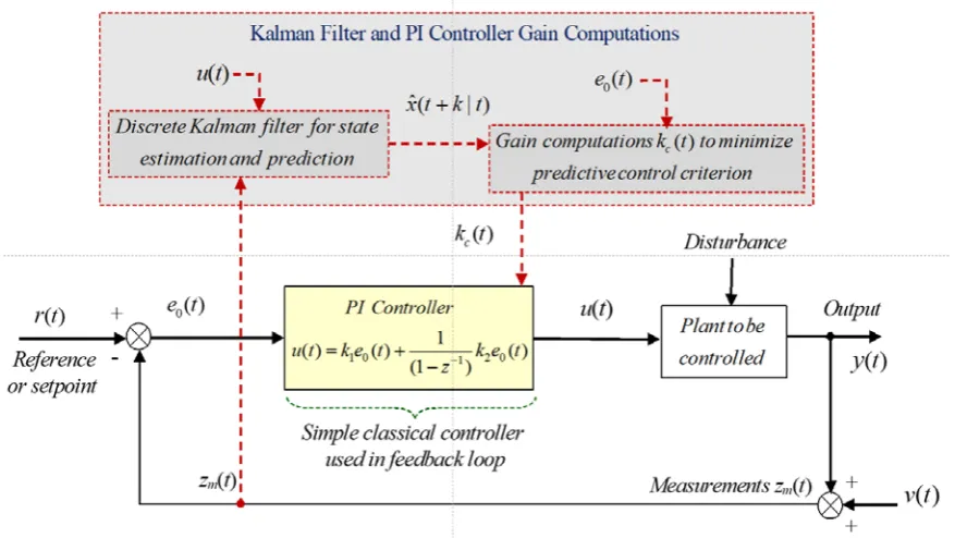
Figure 1. General Strategy of Restricted Structure Predictive Controller

The general philosophy is illustrated in Fig. 1. A low-order controller is chosen like the PI controller shown. A Kalman filter takes measurements and computed controls to determine the state estimates, which are used in an optimization algorithm to find the optimal PI controller gains stored in vector kc(t). The computation of the gains depends upon a receding horizon philosophy. This is different to the usual MPC algorithm since the controller within the loop has a conventional structure and RS-controller gains, rather than future controls, are computed.

2. System Description

The feedback system is shown in Fig. 2. The outputs to be controlled and measured outputs are denoted by y(t) andy t_m( ), respectively. The observations includes measurement noisez_m( )t =y_m( )t +v_m( )t . The stochastic disturbance signals on measured and controlled outputs are represented by linear time-invariant models driven by zero-mean white noise. The deterministic output disturbance terms and reference are denoted

( )

m

The white noise v tm( )is assumed to have a constant covariance matrix = ≥0 T

f f

R R , and

the zero-mean white noise disturbance ξ( )t has an identity covariance matrix. The input sub-system ₁ is assumed stable and has a general operator form, as follows:

(

)( )

(

)( )

−

= k

u t z u t

  (1)

where z I−k denotes a matrix of the common delay elements in the output with k > 0. Let

( ) (

)( )

0 = 1k

u t  _u t and denote the output linear subsystem as _W0=z−k_{W0k, which can} contain any unstable modes. In the initial analysis, the strategy is to first consider the simpler linear problem (where _1k=I) and to then introduce the nonlinear input-subsystem in the last section. The reference r_w(t) is filtered so that r(t) = 1

( )

w

W z− r_w(t),

where 1

( )

w

W z− is an ideal response model, and the error signal e(t) = r(t) – y(t). The

weighted error to be minimized in the cost-function is denoted:

1

c

( ) ( ) ( )

p

e t =P z− e t (2)

where 1

c( )

P z− is a stable proper dynamic cost-weighting. The input to the RS-controller is defined as follows:

e₀( )t =r_w( ) –t z_m( )t (3)

+

Reference

+

C0

r_w

Controller

Input operator subsystem

State-space subsystem

+

Figure 2. RS-GPC System for Unstructured and State-Space Plant Subsystems

2.1 Augmented Linear State-Space Plant Output Subsystem

The first subsystems to be defined is associated with the linear disturbance model and any linear state-space sub-system (denoted W₀) in the plant model. The state-space output subsystem is assumed stabilizable and detectable and is shown in Fig. 3. It includes any disturbance model and cost-function weighting termP z_c( −1). The states, measured outputs, observations and weighted error of the augmented LTI system are given by the augmented system equations as follows:

x t( + =1) Ax t( )+Bu t₀( − +k) D tξ( )+d t_d( ) (4)

0

( ) ( ) ( ) ( )

m m m m

y t =d t +C x t +E u t−k (5)

0

( ) ( ) ( ) ( ) ( )

m m m m m

z t =v t +d t +C x t +E u t−k (6)

0

( ) p( ) ( ) ( )

p p p

e t =d t +C x t +E u t−k

(7)

The signals are explained in more detail and dimensions are listed in Appendix 1.

Fig. 3: Linear Plant Input and State-Space Linear Output and Disturbance Subsystems Observations +

Weighted output

Linear state subsystem dynamics

Disturbance

Control signal

Unstructured plant

+

+ + +

+ +

+

+ +

+ +

Output +

Measurement

noise Delays

2.2 State-Space Prediction Models

The prediction of outputs is required in the later control solution. The future values of

the states and outputs, at time t, may be obtained by repeated use of the state-equation:

x t( + =1) Ax t( )+Bu t₀( − +k) D tξ( )+d t_d( )

Generalising this result, obtain the state at the future timest+i_{, where} i > 0_{, as:}

(

)

1

( ) ( )

(

)

i

i i j

dd j

x t i A x t A− Bu t j k D tξ j d t i

=

+ = +

∑

where the future known disturbance term is given as:

1

( 1) ( 1)

i i j

dd d

j

d t i − d t j

=

+ − =

∑

The future states depend upon the inputs and the state-vector at time t. The expression for the future states may be obtained by changing the time in (8) by the k-steps

of the explicit delay giving:

(

)

1

( ) ( )

(

)

i

i i j

dd j

x t i k A x t k A− Bu t j D tξ j k d t i k

=

+ + = + +

∑

where

1

( 1) ( 1)

i i j

dd d

j

d t i k − d t j k

=

+ + − =

∑

regulated at future times can include any stable dynamic cost-function weighting. Noting (7) it has the following form (fori 1≥ ):

0

( ) _p( ) ( ) ( )

p p p

e t i k+ + =d t i k+ + +C x t i k+ + +E u t i+

( ) ( 1) ( )

p

i

p dd p

d t i k C d t i k C A x t k

(

)

( 1) ( 1) ( )

i

i j

p p

j

C A− Bu t j Dξ t j k E u t i

=

+

∑

Collecting the deterministic disturbance signal terms together:

( ) ( ) ( 1)

pd p p dd

d t+ +i k =d t+ + +i k C d t+ + −i k (12)

Weighted outputs or errors: Noting (11) the weighted outpute t_p( ) becomes:

( ) pd( ) ( )

i

p p

e t+ +i k =d t+ +i k +C A x t+k

(

)

1

( 1) ( 1) ( )

i

i j

p p

j

C A− Bu t j Dξ t j k E u t i

=

+

∑

State Prediction: The i-steps prediction may be written in terms of the future inputs and the estimated state-vector at time t (using (8)) follows as:

0 1

ˆ( | ) ˆ( | )

(

)

i

i i j

dd j

x t i t A x t t A− Bu t j k d t i

=

+ = +

∑

Vector Matrix Notation: Introducing an obvious notation for the error and output signals they may be collected in the N+1 vector form, where N > 0 (Ordys and Clarke 1993) as:

2

( ) ( )

( 1 ) ( 1 )

( 2 ) ( 2 ) ( )

( ) ( ) pd pd pd pd p p p p p p N p p C I

e t k d t k

C A

e t k d t k

e t k d t k C A x t k

e t N k d t N k _{C A}

  + +        _{+ +}   _{+ +}           + +  = + + +_{ } +              _{+ +}  _{ + +} _   _ _    0 0 1 2 0

0 0 0 ( )

0 0 _{( 1)}

0

( 1)

p

p p

N N

p p p

u t

C B _{u t}

C AB C B

u t N C A −B C A − B C B

0

0

0

1 2

0

0 0 0

( ) ( )

0 0

( 1) ( 1 )

( 2)

0

( ) ( 1 )

p p p p p p N N

p p p p

E u t t k

C D

E u t t k

C AD C D

E u t

E u t N C A D C A D C D t N k

ξ ξ ξ − −      +     ₊   _{+ +}           +    + +                +  _ + − + _         _       (15)

This equation (15) may be written as follows:

0

, , ( ) ( ) , ,

P t k N P t k N PN N PN N PN t N PN N t k N

E ₊ =D ₊ +C A x t+ +k C B +E U +C D W₊ (16)

where the matrices are defined by comparison of (15) and (16). These are defined in

Appendix 2. A matrix VPN, for N > 0, may also be defined as follows:

2

1 2

0 0 0

0

0

p

p p

p

PN PN N PN

N

p p

N N

p p p p

E

C B E

C B

V C B E

C A B E

C A B C A B C B E

− − −         = + =                  (17)

For a single-stage criterion the horizon N = 0 and V_PN =E_p. The k steps-ahead tracking

errorEP t k N+ , , includes any dynamic error weighting, and may be written, using (16), as:

0

, , ( ) , ,

P t k N P t k N PN N PN t N PN N t k N

E ₊ =D ₊ +C A x t+ +k V U +C D W₊ (18)

2.3 Linear Prediction Equations

The i-steps ahead prediction of the output may be computed noting (11) and assuming the future values of the control action are known. Let e tˆ (p + +i k t| ) =E e t{ (ˆp + +i k t) | },

then the predicted weighted signal to be minimized, using (13), becomes:

_{0 0}

1

ˆ ( | ) _pd( ) ˆ( | ) ( 1) ( )

i

i i j

p p p p

j

e t i k t d t i k C A x t k t C A− Bu t j E u t i

=

The x tˆ( +k t| ) denotes a least squares state estimate from a Kalman filter, driven by measured outputs (6). Collecting results for the case N≥ 0 the vector of predicted outputs

,

ˆ

P t k N

E ₊ may be obtained in the block matrix form:

,

2

ˆ ( | ) ( )

ˆ ( 1 | ) ( 1 )

ˆ ( 2 | ) ( 2 ) ˆ( | )

ˆ ( | ) ( )

pd

pd

pd

pd

P t k N

p p p p p p N p _p PN N C A D C I

e t k t d t k

C A

e t k t d t k

e t k t d t k C A x t k t

e t N k t d t N k _{C A}

+   + +        _{+ +}   _{+ +}           + +  = + + +_{ } +              _{+ +}  _{ + +} _   _ _      0 0 2 1 2 0 0 ,

0 0 0 _{( )}

0 _{( 1)}

0 ( ) p p p p N p p N N

p p p p

t N

PN PN N PN U

V C B E

E _{u t}

C B E _{u t}

C B

C A B E

u t N

C A B C A B C B E

− − − = +  _{  }  _{  } +  _{  }  _{  } + _     _{  }  _{  + }             _      (20)

This prediction N+1 vector in (20) can clearly be written in the form:

0

, , ,

ˆ _{ˆ( | )}

P t k N P t k N PN N PN t N

E ₊ =D ₊ +C A x t+k t +V U (21)

Output prediction error:

, , ˆ ,

P t k N P t k N P t k N

E ₊ =E ₊ −E ₊

=CPNA x tN ( +k)+V UPN t N0, +CPND WN t k N+ , −(CPNA x tNˆ( +k t| )+V UPN t N0, )

Thence, the inferred output estimation error has the form:

, ( ) ,

P t k N PN N PN N t k N

E ₊ =C A x t +k t +C D W₊ (22)

where the k-steps-ahead state estimation error x t( +k t)=x t( + −k) x tˆ( +k t| ) is

and the expectation of the product of the future values of the control action (assumed known in deriving the prediction equation), and the zero mean white noise driving signals, is null. It follows that EˆP t k N+ , in (21) and the prediction error EP t k N+ , are orthogonal.

2.4 Kalman Estimator

The state estimate x t k tˆ( + | ) may be obtained, k-steps-ahead, in a computationally efficient form from a Kalman filter (Grimble and Johnson, 1988). The number of states in the filter is not increased by the number of the explicit delays k. The estimation equations may be listed as follows:

0

ˆ( 1| ) ˆ( | ) ( ) _d( )

x t+ t =Ax t t +B u t− +k d t (23)

(

)

ˆ( 1| 1) ˆ( 1| ) _{f m}( 1) ˆ_m( 1| )

x t+ t+ =x t+ t +K z t+ −z t+ t (24)

where zˆ (_m t+1| )t =d_m(t+ +1) C x t_mˆ( +1| )t +E u t_{m 0}( + −1 k) (25)

3. Restricted Structure-Generalized Predictive Control

To parameterize the controller a total of Ne linear dynamic functions can be chosen with

different frequency responses. It may be useful to introduce pre and post-compensation matrices, 1

( )

u

L z− and 1

( )

e

L z− , so that the control signal may be expressed as follows:

1 1 1 1 1

0

1 1

( ) ( ) ( , ( )) ( ) ( ) ( )

(

)

N N

u j j e u j j L

j j

e e

u t L z− f z− k t L z− e t L z− f z− k t e t

= =

=

∑

∑

where the weighted input to the RS-controller:

1 1 0

( ) ( ) ( ) ( )( ( ) ( ))

L e e w

e t =L z− e t =L z− r t −z t (27)

The 1

( ) u

weightings are not essential but they may be useful for multivariable systems when diagonal functions are used to simplify (26). The details of the controller parameterization in (26), and the matrices involved, are described in Appendix 3. It is shown that the gains of the controller in the restricted structure controller can be collected in a vector denotedk t_c( ). The RS-controller may then be written in the following form:

1

( ) u( ) e( ) c

u t =L z− F t k (28) The gains might for example, represent the vector of gains in a 3-term PID controller.

3.1 Restricted Structure Controller

There are two methods of implementing the restricted structure controller. The gain can be written in terms of a fixed gain and a deviation. That is, for the optimization procedure the gains can be separated into a constant component kc and a time-varying deviation

( ) c

k t , where the total gain:

k t_c( )=k_c+k t_c( ) (29)

This gives rise to two cases:

1. Letting kc= 0 is what will be termed the absolute control gain case, where the

total controller gains k t_c( )=k t_c( )are to be computed to minimize the criterion.

2. If k_c ≠0 the so-called gain, deviation k tc( ) is to be computed to minimize the

criterion.

If a PID controller structure is chosen, then the first case above is where the total controller gains are to be minimized. The second case can be used when an existing PID

two parallel PID controllers, with one having fixed gains, and one having gain deviations. The RS controller may be written, using (26) and (29) as follows:

1

{

}

{

}

1 1

( ) ( ) ( ) ( ) ( ) ( ) ( )

e e

L L

N N

u j j u j j

j j

u t L z− f z− k e t L z− f z− k e t

= =

=

∑

∑

In terms of the parametrization and the matrix F t_e( )introduced in Appendix 3, the

RS-control follows as:

u t( )=L z_u( −1) ( )F t k_{e c}=L z_u( −1) ( )F t k_{e c}+L z_u( −1) ( ) ( )F t k t_e _c (30)

3.2 Vector of Future Controls

The computation of the controller gains in the next section, based on a predictive control philosophy, provides the gains in a simple manner. This is not the usual approach to predictive control, since it will be assumed that the controller structure is defined in a desired form a priori. A modified receding-horizon philosophy will be invoked. Recall an optimal control signal at time t is based on the receding horizon principle (Kwon and Pearson, 1977), where the optimal control is taken as the first element in vector Ut N0, .

The optimal control is computed for the full horizon but only the value at time t is used.

The equivalent assumption for RS-GPC control is that k t_c( )can be assumed constant in the interval [0, N] and the computed k tc( ) _{can be used to compute the optimal control}

for time t_{. In the spirit of receding control at the next sample time the process can be}

repeated and a new gain can be computed and used to compute the optimal control. With

this assumption the vector of future controls Ut N, may be written, using (83), as follows:

1 1 ,

1

( ) ( ) ( )

( 1) ( ) ( 1)

( )

( ) ( ) ( )

u e

u e

t N c

u e

u t L z F t

u t L z F t

U k t

u t N L z F t N

− −

−

 

 

 

 ₊  ₊

 

 

= =_{ }

 

 

 ₊  ₊

 

   

At each future time the gain in (31) is assumed the same over the prediction horizon. This is different to conventional MPC, where the vector of future controls is computed. The matrix (31) may be denoted U_feand defined as follows:

1 1 1

( ) ( ( ) ( ))T ( ( ) ( 1))T ( ( ) ( ))T T

fe u e u e u e

U t =_ L z− F t L z− F t+  L z− F t+N _ (32)

The vector of future controls for the RS-GPC controller, from (31) and (32):

Ut N, =Uf e( ) ( )t k tc (33)

4. Optimizing the Restricted-Structure Controller

The minimization of a cost-function for a controller of restricted structure, is well established, but the RS problem considered below is unusual. First, there is no approximation in the optimization procedure that occurs in (Grimble, 2004a, 2004b). Secondly, the controller structure is defined in a form where functions are pre-specified and are multiplied by gains that are to be optimized. For the initial results, the unstructured subsystem block is removed by letting_1k =I . It is reintroduced in Section §6. The GPC performance index that motivates the RS-GPC criterion described below, may be expressed as follows (see Clarke et. al. 1987, 1989):

2

0 0

0

{ e ( ) e ( ) ( ) ( )) }

N

T T

p p j

j

J E t j k t j k λ u t j u t j t

=

=

∑

where E{.| } t denotes the conditional expectation, conditioned on measurements up to

time t andλ_jdenotes a scalar control signal weighting. The optimal control signal is to

be calculated for the intervalτ∈[ ,t t+N]. The state-space model generating the tracking error e_p may include any dynamic cost-function weighting ₍ 1₎

c

filter to penalise the low-frequency disturbances. The GPC criterion may be written using the previous definitions of future signals as follows:

{

}

, , , ,

{ _t } _{P t k N}T _{P t k N t N}T _{N t N} |

J =E J t =E E ₊ E ₊ +U Λ U t (35)

The RS-GPC cost-function required here has a term to limit the deviation in gains of the controller that may be added into (35), so that large gain deviations are penalized. In addition to be able to be able to influence the rate of gain variations the difference of the gain deviations may also be costed. The RS-GPC cost-function is defined as follows:

{ }

{

}

T T T T

t P t k N P t k N t N N t N c K c c D c

J =E J t =E E ₊ E ₊ +U Λ U +k t Λ k t + ∆k t Λ ∆k t t (36)

where the gain change deviation:

( ) ( ) ( 1) ( ) ( 1)

c c c c c

k t k t k t k t k t

∆ =  −  − = − − ₍₃₇₎

The terms in the criterion may be summarized as follows:

• The cost-weightings on the future inputs u₀ are defined as:

2 2 2 2

0 1

{ , ,..., }

N diag λ λ λN

Λ = .

• The cost-weightings on the deviations in controller gains are defined as:

2 2 2 2

0 1

{ , ,..., } e

K diag ρ ρ ρN

Λ = .

• The cost-weighting on the deviations in the difference of the gains is denoted:

2 2 2 2

0 1

{ , ,..., } e

D diag γ γ γN

Λ = .

Implementing the controller gains in the parallel form in (29) can be interpreted as the first term being a fixed controller and the second term (having optimal deviation gains) as providing adaption to reference or disturbance signal changes. The cost-function (36)

includes a penalty on the gain deviations k t_c( ) and their rate of change∆k t_c( ). The two methods of implementing the controller gains will not therefore lead to the same results. For example, assuming the fixed component of the controller is stabilizing and increasing

the penalty on k t_c( )will result in the fixed controller performance being approached.

4.1 Cost-Function Minimization

The vector of future errors can be replaced by orthogonal predicted errors and estimation error terms. From equation (36) obtain the criterion as follows:

0 2 0

, , , , , ,

ˆ ˆ

( ) ( )

{

P t k N P t k N P t k N P t k N t N N t N

J =E E ₊ +E ₊ E ₊ +E ₊ +U Λ U

2 2

( ) ( ) ( ) ( ) |

}

T T

c K c c D c

k t k t k t k t t

+ Λ  + ∆ Λ ∆ ₍₃₈₎

The terms in the cost-index can be simplified by using the orthogonality of the optimal estimate Eˆ_{P t k N+ ,} and the estimation errorE_{P t k N+ ,} . Simplifying the expression,

0 2 0 2 2

, , , , 0

ˆT ˆ T T_{( ) ( )} T_{( ) ( ) ( )}

P t k N P t k N t N N t N c K c c D c

J =E ₊ E ₊ +U Λ U +k t Λ k t + ∆k t Λ ∆k t +J t (39)

where E_{P t k N+ ,} =C_PNA x t_N( +k t)+C D W_{PN N t k N+ ,} andthe cost-term J t₀( )=E E{T_{P t k N+ ,} E_{P t k N+ ,} | }t

is independent of the control. Noting (21) the vector of state-estimates may be written as follows:

0 0

, , , , ,

ˆ _{ˆ( | )}

P t k N P t k N PN N PN t N P t k N PN t N

E ₊ =D ₊ +C A x t+k t +V U =D ₊ +V U (40)

, , ˆ( | )

P t k N P t k N PN N

D ₊ =D ₊ +C A x t+k t (41)

The state-estimate x tˆ( +k t| ) only depends upon past values of the control signal. The multi-step cost-function (39) may therefore be expanded as follows:

0 0 0 2 0

, , , , , ,

( _{P t k N PN t N}) (T _{P t k N PN t N}) _{t N}T _{N t N}

J = D ₊ +V U D ₊ +V U +U Λ U

2 2

0

( ) ( ) ( ) ( ) ( )

T T

c K c c D c

k t k t k t k t J t

+ Λ  + ∆ Λ ∆ +

(

)

0 0 0 2 0

, , , , , , , ,

T T T T T T

P t k N P t k N t N PN P t k N P t k N PN t N t N PN PN N t N

D ₊ D ₊ U V D ₊ D ₊ V U U V V U

=   +  +  + + Λ

2 2

0

( ) ( ) ( ) ( ) ( )

T T

c K c c D c

k t k t k t k t J t

+ Λ  + ∆ Λ ∆ + ₍₄₂₎

Before performing the optimization, the controller structure will be defined to have the

desired restricted structure form. From (29) k t_c( )= +k_c k t_c( ) and from (37) the change

in gain∆k tc( )=k tc( )−k tc( −1). Recall in this section is1k =I , so that

0

, ,

t N t N

U =U , where

, ( ) ( )

t N f e c

U =U t k t . Substituting the cost-function (42) may now be expanded as below:

(

)

, , ( ) , , ( ) ( ) ( ) ( )

T T T T T T T T

Pt k N Pt k N c f e PN Pt k N Pt k N PN fe c c f e PN PN N fe c

J=D ₊ D ₊ +k t U V D ₊ +D ₊ V U k t +k t U V V + Λ U k t

2 2 2 2

( ) ( ) ( 1) ( ) ( ) ( 1)

T T T T

c K c c K c c D c c D c

k k t k t k k t k t k t k t

− Λ − Λ − − Λ − Λ −

2 2 2 2

0

( )( ) ( ) ( 1) ( 1)

T T T

c K D c c K c c D c

k t k t k k k t k t J

+ Λ + Λ + Λ + − Λ − +

The equations can be simplified by defining:

2 2 2

( )

T T

N f e PN PN N f e K D

X =U V V + Λ U + Λ + Λ (43)

CN

T T f e PN

CN

T T

PN N fe PN PN N

C_φ =P C A =U V C A (45)

Substituting for these system matrices, the following expression is obtained:

, , ( ) CN , , CN ( )

T T T T

P t k N P t k N c P t k N P t k N c

J =D ₊ D ₊ +k t P D ₊ +D ₊ P k t

2 _{( ) ( )} 2 _{( 1)} 2 _{( ) ( )} 2 _{( 1)}

T T T T

c K c c K c c D c c D c

k k t k t k k t k t k t k t

− Λ − Λ − − Λ − Λ −

(

)

0

( ) ( ) ( ) ( 1) ( 1)

T T T T T

c f e PN PN N fe K D c c K c c D c

k t U V V U k t k k k t k t J

+ + Λ + Λ + Λ + Λ + − Λ − +

, , ( ) CN , , CN ( )

T T T T

P t k N P t k N c P t k N P t k N c

D ₊ D ₊ k t P D ₊ D ₊ P k t

=   +  + 

(

)

(

)

0

( 1) ( ) ( ) ( 1) ( ) ( )

T T T T

c K c D c c K c D c c N c

k k t k t k t k k t k t X k t J

− Λ + − Λ − Λ + Λ − + +

Let the signal ψ(t) be defined to simplify this equation:

ψ( )t = −Λ_K2 k_c− Λ2_{D c}k t( −1) (46)

The cost-function expression becomes:

, , ( ) CN , , CN ( )

T T T T

P t k N P t k N c P t k N P t k N c

J =D ₊ D ₊ +k t P D ₊ +D ₊ P k t

+ψ( )t Tk t_c( )+k_cT( )tψ( )t +k_cT( )t X k t_{N c}( )+J₀ (47)

where J₀ =k_cTΛ2_Kk_c+k_cT(t− Λ1) 2_{D c}k t( − +1) J₀ (48)

future optimal controls (Grimble and Johnson, 1988). Noting the J₀ term is independent

of the control action, the vector of optimal gains becomes:

(

) (

)

, ( )

( ) ( ) CN

T T

c f e PN PN N f e K D P t k N

k t = − U V V + Λ U + Λ + Λ − P D ₊ +ψ t (49)

Also recall from (41) and (45),

(

)

0

, CN , CN , ˆ( | )

P t k N P t k N P t k N PN N

D ₊ =P D ₊ =P D ₊ +C A x t+k t (50)

Thus, the optimal gains in (49) can be simplified further as follows:

1

(

)

( ) ( )

c N P t k N

k t = −X− D ₊ +ψ t (51)

where

0

, CN , ˆ( | )

P t k N P t k N

D ₊ =P D ₊ +C x t_φ +k t (52)

Asymptotic behaviour

Observe from (49) that if 2

D I

Λ → ∞ × the limiting gain k t_c( )=k t_c( −1)and the gains

become constant. Similarly, if 2

K I

Λ → ∞ × the limiting gain k t_c( )=k_c and the gains

become equal to the constant initial PID gain settings. Minimum-cost

Substituting in (47) for 0 , ,

T T

Pt k N f e PN Pt k N

D ₊ =U V D ₊ , using (52) and substituting for the gain

( )

c

k t in (51), the minimum-cost becomes:

(

) (

)

, , , ( ) , ( ) 0

T T

min P t k N P t k N P t k N N P t k N

T

J =D ₊ D ₊ − D ₊ +ψ t X− D ₊ +ψ t +J (53)

where 2 2

0 ( 1) ( 1) 0

T T

c K c c D c

Theorem 1: Restricted Structure-Generalized Predictive Controller

Consider the linear system and assumptions introduced in §2, where the sub-system

=

1k I

 . The restricted structure generalized predictive controller is required to

minimize the following cost-index:

J =E J{ }_t =E E

{

}

The RS-GPC _{controller can be implemented as follows:}

1 1 1

1

( ) ( )

(

)

N

u j j L u c

j e

e

u t L z− f z− k t e t L z− F t k t

=

=

∑

where the functions f_j

(

)

structure, and where 1

0

( ) ( ) ( )

L e

e t =L z− e t . The block-diagonal matrix F t_e( )has the form:

{

}

( ) _f ( ) _f ( ) _fm( )

e

F t =diag e t e t  e t (56)

where for each i ={1, 2 ,…,m} the row vector e_{f i}( )t = f_ei1 f_ei2  f_ei r_, and these

functions are pre-specified by the designer. The optimal feedback controller gains are chosen to minimize (54). By invoking a form of the receding horizon philosophy, the

RS-GPC optimal time-varying gains satisfy:

(

)

1 0 2 2

,

( ) ( 1)

c N P t k N K c D c

k t = −X− D + − Λ k − Λ k t−

(

)

1

, ˆ( | ) ( )

CN

N P t k N

X− P D ₊ C x t_φ k t ψ t

= − + + + (57)

where the matrices ψ( )t = −Λ2_Kk_c− Λ2_{D c}k t( −1), X_N =U_{f e}T(V V_PNT _PN + Λ_N2)U_{f e}+ Λ + Λ_K2 2_D, and

CN

T T f e PN

1 2

11 12 21 22 1 2

1 2

T T T

T

T T T T T r T T r m T m T m r

c c c c m c c c c c c c c c

channel 1 gains channel 2 gains channel m gains

k k k k k k k k k k k k k

      =_{  }=            (58)

The vector of future controls may be obtained as:

, ( ) ( )

t N f e c

U =U t k t (59)

where 1 1 1

( ) ( ( ) ( )) ( ( ) ( 1)) ( ( ) ( )) T

T T T T

f e u e u e u e

U t =_ L z− F t L z− F t+  L z− F t+N _ ● Solution: The RS-GPC proof follows by collecting the results above. ●

Controller Background Gain Computations

Disturbance

Reference

Plant

Output

( )t

y

( )t

ξ

RS-GPC: Functional controller subsystem

u(t)

ˆ( | ) x t t

Kalman filter and PID gain computation Function error terms

+ + Observations z(t)

1

0( )

W z−

v

1 1 0 1 2 0 1 3 0

1 (1 )

( ) ( ) ( ) ( ) (1 ) (1 ) Extended PID Restricted StructureController

z u t k e t k e t k e t

z αz

− − − − = + + − − e L ( ) c k t ( ) e F t

(

)

1 2 2

, ˆ

( ) _CN ( | ) ( ( 1))

c N P t k N K c D c

k t = −X− P D + +C x tφ +k t − Λ k + Λ k t−

{

}

s s sr

fs e e e

e f f f m

e

e t L z e t

e t f f f

F t diag e t e t e t − =   =   =  

0( )

e t

pd

d z(t)

+

- ( )t

r

( ) ( )c

e

F t k t

( )

L

e t Gain computations

d d d u L Figure 4. RS-GPC State-Space Controller Structure

Comments on the Form of the solution

solutions. The theory applies for any RS controller, which can be represented by a summation of transfer-function terms multiplied by gains.

Numerical robustness

The solution for the RS-GPC optimal control (57) depends upon the inverse of X_N. This time-varying matrix is full-rank because of the cost-weighting definitions. The expression for the gain-vector is similar to the vector of future controls in the usual GPC

solution. However, the denominator matrix in (57) will often be of lower dimension. The weightings 2

K

Λ and 2

D

Λ depend on the number of the RS-controller gains and they ensure

thatX_Ndoes not become singular. The gains are not penalized in the cost-functions of traditional model predictive controls. However, it is valuable to be able to cost and tune these gains, and avoid numerical problems with near singularX_N.

4.2 Square of Sum Optimization Problem

The problem considered here is a special cost-minimization control problem, which is needed to motivate a nonlinear predictive controlproblem introduced later. The solution is obtained by completing the squares in Appendix 4.

Theorem 2: Equivalent Cost-Minimization Problem

Consider the system and assumptions introduced in §2, where the input subsystem

=

1k I

 and the minimization of the RS-GPC cost-index (36), where the vector of

optimal RS-GPC controls is given by (51). Let a multi-step cost-index be defined as follows:

, ,

( ) { T_{P t kN P t kN} | }

J t = ΦE ₊ Φ ₊ t (60)

,

0 0 1 2

, CN , CN N CN ( ) CN ( )

Pt k+ N P EPt k N+ F Ut F k tc F k tc

Let the weightings CN

T T f e PN

P =U V , CN0 2

T f e N

F =U Λ ,F_CN1 = Λ2_K, F_CN2 = Λ_D2 and V_PN =C_PNB_N +E_PN,

and define X_N =UT_{f e}(V V_PNT _PN + Λ2_N)U_{f e}+ Λ + Λ_K2 2_D. Then the vector of optimal gains

becomes:

k tc( ) XN1

(

)

−

+

= − + + − Λ − Λ − (62)

whereC_φ =U V CT_{fe PN}T _PNA_N and ψ( )t = −Λ_K2 k_c− Λ_{D c}2k t( −1). This expression for the gain vector is identical to the RS-GPC controller in (51) or Theorem 1. The optimal control can be realized as in shown in Fig. 5. The vector of future controls is given as follows:

, ( ) ( )

t N f e c

U =U t k t

or

(

)

1 0

, ,

( )

t N f e N P t k N

U = −U X− D ₊

+

t

Solution: The proof follows by collecting results in Appendix 4. ■

Figure 5. RS-GPC State-Space Controller Structure Disturbance Reference Parameterized controller gains×signals Output

( )t

y

ξ

Feedback controller subsystem

u(t)

ˆ( | ) x t t

Kalman Filter Stage and Controller Gain Calculation

Function error terms

+ + Observations z(t)

0

W

v × F t k te( ) ( )c

( )

e

F t 0( )

e t

, _d, _pd d d d z(t)

+

- ( )t

r Linear plant ( ) c k t

{

}

s s sr

f s e e e

e f f fm

e

e t L z e t

e t f f f

F t diag e t e t e t

− =   =   =   1 ( ) u

L z−

(

)

1 0 ,

( ) ( )

c N P t k N

4.3 Cost-Function Tuning Variables

Retuning the controller should be simple. For a scalar problem, the weighting on the control signal provides a simple way to vary the speed of response of the system. The weighting on the error can be chosen to be unity. In this case, or if integral action is included, then the integrator weighting gain can be scaled to unity. The remaining weightings 1 2

CN K

F = Λ and 2 2

CN D

F = Λ are on the magnitude of the gains and rate of gain changes. The cost of control is a term introduced by Isaac Horowitz to drew attention to the cost of feedback. High gains have disadvantages and the ability to reduce these gains whilst not sacrificing performance is valuable, providing the control action is satisfactory.

4.4 Stability

The fact that the solution provides an optimal control does not of course guarantee stability. If the system has no disturbance or reference changes, then from (62), the RS-controller gains become constant and the stability conditions are those for a linear time-invariant system, and the characteristic polynomial can be inspected. Under more general changing conditions, the system is time-varying. Nevertheless, if the rate of change of gains is controlled and the gains vary sufficiently slowly, it should be possible to establish stability conditions using similar analysis to that for adaptive systems. However, if hard constraints on controller gains are applied the region of operation is well defined. The

approach of Dıaz-Rodrıguez and Bhattacharyya (2016) defines a stabilizing set of PI (or

PID) controllers for such systems. The definition of the cost-function weightings is important since they determine performance and stability (illustrated in the example).

5. SI Automotive Engine Design

Figure 6. Engine Model: Inputs, Outputs and Parameters

The original control problem involved engine idle speed control by manipulating the throttle input, subject to a varying load torque. The control objective here is to keep the engine speed at the set-point irrespective of the load torque disturbance. For comparison purposes, a PI-controller with an anti-windup mechanism is included. A speed set-point signal (in rpm) is to be tracked, in the presence of load torque. The controller computes the necessary throttle angle based on the desired rpm and the measured engine speed, which is the output of the vehicle dynamics subsystem.

Model Equations

The equations for various engine model subsystems follow. The signals under consideration are as follows:

• controlled output: engine speed N (rpm)

• measurements: engine speed and intake manifold pressure P_im (bar)

• control input: throttle angle  (deg.)

• unknown varying disturbance input: load torque T_load (Nm)

• known input: spark advance SA (deg.).

Throttle flow: m_asgn_f f( )  (p_r) where

1, 0, 1,

a m

f a m

a m

P P

sgn P P

P P

 

 

_ 

 



(flow direction)

Engine

Model Throttle

Load torque

Spark

Speed

Engine torque

MAF

Charge

2 3

( ) 2.821 0.05231 0.10299 0.00063

f         (discharge coefficient)

( ), ( )

r m a a m

p min P P P P (pressure ratio)

2 (1 ), 0.5

( )

(sonic flow)

1.0 0.5

r r r

r

r

p p p

p

p

  

   _



 and atmospheric pressure is set to Pa = 1 bar.

Intake manifold pressure: _m





m

RT

P m f P N

V

 

 _{ where RT/Vm=0.41328 and}

2 2

( , ) 0.366 0.08979 0.0337 0.0001

pump m m m m

f P N      P N  N P   P N (pumping)

Air charge: 2

0.0001 0.1812 _m 0.0725 _m 0.0005 _m 0.0362

CAC   N P  P  P  N

Power stroke delay: This parameter defines the variable time delay affecting the air charge delivered for combustion, tdel  N .

Engine torque: T_eng  f_TQ(CAC CFC SA N, , , ) where,

2

2 2 2

( , , , ) 181.3 379.36 21.91 0.85 0.26

0.0028 0.027 0.000107 0.00048 2.55 0.05

TQ

f CAC AFR SA N CAC AFR AFR SA

SA N N N SA SA CAC SA CAC

          

              

The stoichiometric air-fuel ratio (AFR) is assumed AFR = 14.6.

Vehicle dynamics: N (1 J T)





5.1 Design Aspects

The control problem is to manipulate the throttle angle to track the engine speed set-point subject to unknown drag/load torque variations. The test scenarios involve speed set-point step changes from 2000 to 2500 rpm, and load torque varying between 20 to 25 Nm. Let the prediction-horizon N = 20 and delay k = 1. The cost weightings:

2

N

Λ =400.I, Λ2_D = 1e10×diag{1 0.1 1}, Λ2_K= 1e9×diag{12 1 0.1},

1 1

(1 - 0.98z / )

0.25 ) (1

c

P = × − −z− and 1

c

1_{) 100 30 ) / (1 0.1} 1₎

( (

k z z z

− _{= −} − ₋ −

The frequency response of the weighting on control is shown in Fig. 7 and the error weighting multiplied by the plant transfer function (between throttle angle (degrees) and speed (rpm)). The plots cross at about 2 radians per second and the rule of thumb is that the bandwidth should be in the region of 0.5 seconds.

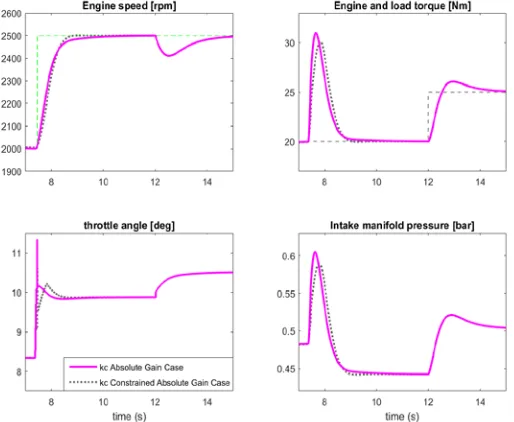
The step-responses shown in Fig. 8 are for the two RS cases of using absolute gains or gain deviations, and final response is for the use of MPC. In this latter case a

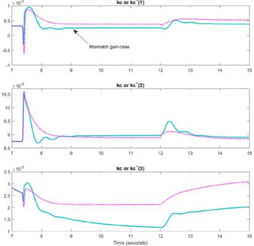
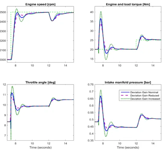
Generalized Predictive Control algorithm was used as in Ordys and Clarke (1993). None of the methods is clearly preferable, since it is likely similar results can be obtained by different weightings. This does not apply to the constrained gain cases where the particular problem may dictate the best choice. The gains in Fig. 9 indicate the gains only change when disturbances or reference changes occur.

Figure 7. Weighting Frequency Responses Plant × Pc and Fc

Comparison with Fixed PID

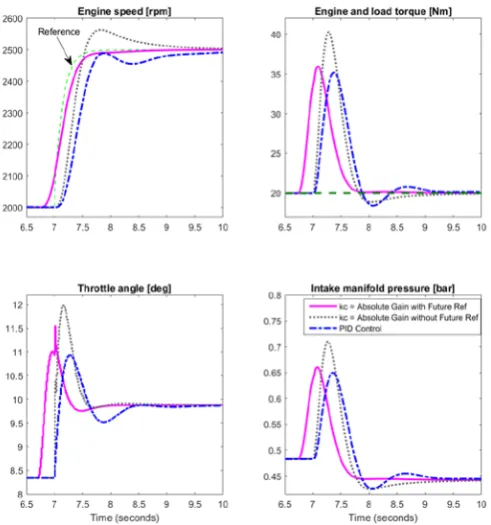
The results shown in Fig. 10 compare the absolute gain case against a traditional PID

Figure 8. Comparison of Time Responses for RS-Absolute and Gain Deviation Cases, and MPC Design (No Reference Knowledge, Gain Constraint, Rate of Change Weight)

Figure 9. Comparison of Responses of Gains for Absolute and Gain Deviation Cases

8 10 12 14 2000

2100 2200 2300 2400 2500 2600

Engine speed [rpm]

8 10 12 14 20

25 30 35

Engine and load torque [Nm]

8 10 12 14 Time (seconds)

8.5 9 9.5

10 10.5

11 11.5

Throttle angle [deg]

Response Absolute Gain Response Incremental Gain Response MPC Case

8 10 12 14 Time (seconds)

0.4 0.45 0.5 0.55 0.6 0.65 0.7

Intake manifold pressure [bar]

Speed reference

Using incremental gains

Using absolute gains Using MPC

Load change

7 8 9 10 11 12 13 14 15

2 4 6 8 10

10-4 Gains for Absolute or Deviation Cases kc (1)

7 8 9 10 11 12 13 14 15

-5 0 5 10 15

10-5 Gains for Absolute or Deviation Cases kc (2)

7 8 9 10 11 12 13 14 15

Time (seconds) 1.5

2 2.5

3 3.5

10-3 Gains for Absolute or Deviation Cases kc (3)

Figure 10. Comparison with PID Including of RS-GPC with Absolute Gains Effect of gain constraints

For the case of constrained gain magnitudes let the constraints be set as: kmax = [4 2e-3 5e-2e-3]T, kmin= [0 0.5e-5 1e-5]T, ∆kmax = [1 1 1]T, ∆kmin = [-1 -1 -1]T. A comparison of the time-responses for the unconstrained and constrained cases using absolute gains are shown in Fig. 11. The gains in Fig. 12, show the constraints are active.