Spectral-spatial Classification of Hyperspectral Data
Using Spectral-domain Local Binary Patterns
WANG Cailing1,*, Jinchang Ren2, WANG Hong-wei3, Yinyong Zhang2, WEN Jia4
1. Xi’an Shiyou University, School of computer science, Xi’an 710065, China 2. Department of electronic and electrical Engineering, University of Strathclyde, UK
3. Engineering University of CAPF,Xi’an,710086, China;
4. School of electronics Engineering, Tianjin Polytechnic University, Tianjin,300387,China;
Abstract- It is of great interest in spectral-spatial features classification for hyperspectral
images (HSI) with high spatial resolution. This paper presents a novel Spectral-spatial
classification method for improving hyperspectral image classification accuracy.
Specifically, a new texture feature extraction algorithm exploits spatial texture feature
from spectrum is proposed. It employs local binary patterns (LBPs) in order to extract
the image texture feature with respect to spectrum information diversity (SID) to
measure the differences of spectrum information. The classifier adopted in this work is
support vector machine (SVM) because of its outstanding classification performances.
In this paper, two real hyperspectral image datasets are used for testing the performance
of the proposed method. Our experimental results from real hyperspectral images
indicate that the proposed framework can enhance the classification accuracy compare
to traditional alternatives.
Key Words-Hyperspectral image classification; spectral-spatial analysis; local binary
patterns; spectrum information diversity; support vector machine.1
I Introduction
Hyperspectral image (HSI) captures reflectance values from Visible to Infrared spectrum
Received: Accepted:
Foundation: National Natural Science foundations of China ( Grant Nos. 41301382, 61401439, 41604113, 41711530128 ) and foundation of Key lab of spectral imaging, Xi’an Institute of Optics and Precision Mechanics of CAS.
which covers a wide spectral range with hundreds of bands for each pixel in the image. This rich
spectral information provides possibility to distinguish different materials spectrally. HSI
classification plays an important role in hyperspectral image application, such as crop analysis,
plant and mineral identification, among others.
In traditional HSI classification systems, classifiers are only able to consider spectral
signatures without considering the correlations between the pixel of interest and its neighboring
pixels1 , 2 , 3 . Numerous classification techniques for HSI have been developed such as
K-nearest-neighbor (K-NN) classifier4 , maximum-likelihood estimation (MLE)5, artificial neural
networks6, kernel-based techniques7. In particular, support vector machines 8(SVMs) have
demonstrated excellent performance for HSI classification. However, it is a very challenging task
due to the tiny distinction among spectral signatures of various types in same families, such as
tillage in the corn fields. Meanwhile the spatial resolution is increasing during last decades, it is of
great interest in exploiting spectral-spatial proposing to improve the accuracy of HSI
classification9, 10.
There are some spectral-spatial classifiers developed for Features-level fusion. For example,
Generalized Composite Kernel (GCK) for combination of both spectral and spatial information
were employed by multinomial logistic regression and support vector machine are introduced
in[10] and[11]. In addition to the composite classifier framework, many researches focus on
spatial feature extraction. For instance, morphological profiles [MPs]12 and attribute profiles [APs]
13have been successfully employed to model structural information in hyperspectral image
processing. Local binary pattern operator, which extract texture feature in spatial domain, is also
pre-processing are present in literature.
As we all know, the texture feature is one of the key feature to display image characteristics.
A batch of algorithms including gray-level co-occurrence matrix (GLCM), Gabor texture features,
gradient orientation features and local binary pattern operator (LBP) are proposed to extract image
texture feature such as edges, corners, and knots. Hashing methods1819,20,21, which encode
high-dimensional image descriptors as compact binary strings, can be considered as new feature to
be used for HSI classification. The conventional LBP is a simple yet efficient advanced operator to
describe local spatial pattern by binary threshold with the center pixel value. In recent years, LBP
has been widely used in image classification22 and detection23. It has been proposed to be used in
hyperspectral image classification recently. In [15], the LBP and Global Gabor filter(GGF) are
employed to extract spatial texture information in a set of selected bands firstly, then the
feature-level fusion and decision-level fusion are investigated on the extracted multiple features.
Feature-level fusion combines different feature vectors together into a single feature vector.
Decision-level fusion performs on probability outputs of each individual classification pipeline
and combines the distinct decisions into a final one with the LOGP. Unfortunately, the LBP texture
feature is extracted by calculating the histogram of local region, therefore, the time-consumption
will increases rapidly with bands number increases. In order to overcome classification problem
above in HSI, a new texture feature extraction algorithm which exploits spatial texture feature
from spectrum domain is proposed in this paper. The proposed classification method can extract
the texture feature using the algorithm proposed in this paper, then, the extracted spatial features
of central pixel can be stacked with its spectral features to develop a discriminative classifier.
extraction-based classification and the algorithm proposed in this paper, the proposed texture
feature extraction leads to a substantial improvement in classification performance and
time-consuming.
The structure of this paper is organized as follows. In section 2, we briefly introduces the
previous related researches. In section 3, the proposed mathematical texture feature extraction is
discussed. Section 4 provides a detailed description of the proposed classification method and also
shows classification results using the real HSI. Finally, Section 5 concludes this paper with some
remarks.
2. Related Work
In this section, we briefly review the conventional LBP method and SVM classifier.
A. A Review of LBP
Local binary pattern (LBP)24 measures a local neighborhood around each central pixel
whether the central pixel has a larger intensity value or not firstly, then generate a binary code for
summarizing local gray-level structure. The basic LBP method considers a small circularly a small
circularly symmetric neighborhood as
P
, along with selected neighbors{ }
P01 i it
and centralpixel
t
c.The LBP is computed by:
1
, ( ) 0
(
)2
1,
0
( )
0,
0
c
P
i
P R t i c
i
LBP
s t
t
x
s x
x
(1)
After forming an LBP code image for each band of hyperspectral image, the texture feature
formed as the LBP histogram is generated for each local patch centered at a pixel of interest. The
time-consumption will go up rapidly with the bands number increase. To solve this problem, band
selection algorithm are adopted firstly and the texture feature based on LBP is extracted from the
selected bands. The PCA is most popular algorithm for dimension reduction and first one to three PC
images are employed to the spatial feature extraction. Although the PCA method seems reasonable
because the selected bands images are optimal for data representation, it should be noted that some
important information is still contained in some other image bands.
B. SVM classifier
There are many principles to distribute the data points to a model. One of the most popular
classification methods is support vector machine (SVM)25, which is often employed for HSI image
classification. The key idea behind a kernel version of SVM is to map the data from its original
input space into a high-dimensional kernel-induced feature space where classes may become more
separable. SVM model is constructed on determining an optimal hyper-plane in the kernel-induced
space by solving
2
, , 1
1
min
2
in i
p i
(2)Subject to the constraints:
,
1
i i i
y
x
p
(3)For
i
0
andi
1,...,
n
, where
is normal to the optimal decision hyper-plane (i.e.
,
X
p
0
),n
denotes the number of samples,p
is the bias term,
is the regularization parameter which controls the generalization capacity of SVM, and
iis theThe problem above can be solved by introducing Lagrange multipliers with slack variables
and regularization form
1 , 1
1
max
,
2
n n
i i j i j i j
i i j
a
a a y y K x x
(4)Where
a a
1, ,...,
2a
n are nonzero Lagrange multipliers constrained to0
a
1
, and1
0
n i i ia y
There are some commonly implemented kernel functions like the polynomial kernel and the
RBF kernel. In this paper, RBF is considered and it is represented as
,
exp
2
2 2i j
i j
x
x
K x x
(5)Finally, the decision function is represented as
1
sgn
n i i i,
i
f x
y a K x x
p
(6)3 Texture feature for Hyperspectral image
A. Extended LBP with Respect to SID
To calculate spectrum-based LBP, we need to calculate the similarity firstly. In this paper, the
Spectral information divergence (SID)26 is employed to quantify differences between reflectance
spectrums in both magnitude and direction dimensions. Some other similarity methods for two
spectrums are also used in this step such as Spectral angle Cosine, etc.
Assume that hyperspectral pixel
X
( , , , )
x x
1 2
x
L , each componentx
l is the pixel of bandB
l acquired at a particular wavelength
l .{ }
L1l l
is a set ofL
wavelengths. Supposex
as a random variable by defining an appropriate probability space( , , )
P
associated with1 2
( ,
, ,
L)
P
p p
p
forx
by1
({ })
ll l L
l l
x
P
p
x
(7)Denoted another hyperspectral pixel
Y
( , , ,
y y
1 2
y
L)
with probabilityQ
( , , , )
q q
1 2
q
L , vector SID is calculated by Eq. (3).( , )
(
)
(
)
SID X Y
D X Y
D Y X
(8)Where
1
(
)
Llog( )
l ll l
p
D X Y
p
q
Supposed that central hyperspectral pixel is
X
c and the neighborhood hyperspectral pixelsis
{ , , , }
Y Y
1 2
Y
N , WhichN
is the number of neighborhood pixels. The threshold for binary ischosen by calculating the Mean of SID, shown in Eq. (4).
1
1
(
, )
N
c c n
n
SID X Y
N
(9)Then the SID_LBP is shown in Eq. (5)
1
1 , ( )
0
(
( , )
)2
1,
0
( )
0,
0
c N nN R X n c
n
LBP
s SID X Y
x
s x
x
(10)B. Texture Feature extraction by SID-LBP
Traditional texture feature extraction on LBP is generated for the center pixels by calculating
the histograms in its corresponding local LBP image patch. The texture feature extraction on
SID_LBP is also done by histograms in its corresponding local LBP image patch.
Note that patch size is a user-defined parameter, and the various patch sizes will affect the
final classification accuracy.
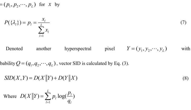
[image:7.595.104.507.78.311.2]feature extraction. Fig.1 (a) gives the implementation of LBP feature extraction applied to each
selected band image. Fig.1 (b) gives the SID-LBP features extraction.
HighSpectral Image Datecube (145X145X200)
Selected Bands Images LBP images of Selected Bands images LBP Image Patch LBP Histogram
LBP Histogram LBP Image Patch
LBP images of Datacube HighSpectral Image
Datecube (145X145X200)
Band Selection
Method
LBP Operator
[image:8.595.100.486.134.357.2]SID_LBP Operator
Figure 1 Comparison on implementation of traditional LBP and SID-LBP feature extraction. (a) Implementation of traditional LBP feature extraction. (b) Implementation of SID-LBP feature extraction
Compared to the conventional LBP-based classification framework, there are three main
advantages on SID_LBP process. Firstly, the proposed SID_LBP texture feature extraction is done
on original data cube which the total bands information are considered without any band selection
methods, therefore, there is less time-consuming and less information loss. Secondly, the
histogram operator obtained from each LBP image patch of every selected band image in
traditional LBP feature method which the computation time will increased rapidly with the bands
image number and LBP image patch size, however, the histogram calculation is only done on one
image in SID_LBP operator, therefore, SID_LBP method has higher accuracy than one band
selection for traditional LBP feature method and less time-consuming than multi-bands selection
of traditional LBP feature. Thirdly, as all LBP histograms are stacked as texture feature for
classification, the spatial feature dimensions will increase rapidly with the number of selected
LBP histogram is produced.
In this paper, a novel classification method is proposed, which consists of spatial texture
feature by SID_LBP and classification step. The procedure is as follows.
Algorithm: SID_LBP_SVM classification
Input: Training set with N samples for each class and texture patch size sets W
Output: Classification maps and accuracy
1Calculate the texture feature histograms at window W by SID_LBP
2 Calculate spectral channel features
3 Normalize, stack and reduce spatial-spectral features
4 Train a classification model
5Classify the test set and assess accuracy
6 Return the classification maps and accuracy
4. Experimental Results
A. Data Sets
In this section, we evaluate the proposed approach using two real HSI data sets. These data
sets include different contexts, different spatial resolutions and different bands in order to assess
the performance of proposed approach.
The first data was collected by Airborne Visible/Infrared Image Spectrometer (AVIRIS) over
Northwest Indiana, Indiana, USA, in June 1992. The image presents a classification scenario with
the spatial coverage of
145 145
pixels covering 16 classes of different crops at 20-m spatialresolution and 220 bands in 0.4 to 2.45
m
region of visible and infrared spectrum. AfterThe second data set was collected by the Reflective Optics System Imaging Spectrometer
sensor covering the city of Pavia, Italy. The data set consists of 115 spectral bands with
610 340
pixels covering 9 classes with a spectral range from 0.43 to 0.86
m
and spatialresolution of 1.3m. After removing 12 noisy channels, the remaining 103 bands were used for the
test.
All the datasets present the challenging classification scenarios. The class information of
three images is detailed in Table 1, Table2, and Fig.1 and Fig.2.
Table 1
The class information of Indian Pines Data set
Order Class name Number of
samples
1 Alfalfa 54
2 Corn-notill 1034
3 Corn-mintill 834
4 Corn 234
5 Grass-pasture 497
6 Grass-trees 747
7 Grass-pasture-mowed 26
8 Hay-windrowed 489
9 Oats 20
10 Soybean-notill 968
11 Soybean-mintill 2468
12 Soybean-clean 614
13 Wheat 212
14 Woods 1294
15 Building-grass-trees-drives 380
16 Stone-steel-towers 95
Total 10366
Table 2
The class information of Pavia Data set
Order Class name Number of
samples
1 Asphalt 6631
2 Meadows 18649
3 Gravel 2099
4 Trees 3064
5 Metalsheets 1345
6 Bare soil 5029
7 Bitumen 1330
8 Bricks 3682
9 shadow 947
(a) (b) (c) (d) Figure 2.The 10th band of Indian Pine image; (b) Indian Pine ground survey; (c)10% training pixels;(d) 90% test pixels
训练样本集 测试样本集
(a) (b) (c) (d)
Figure 3.(a)The 10th band of the University of Pavia;(b) the University of Pavia ground survey(c)10% training pixels;(d) 90%
test pixels
B. Experimental Setup
In order to show the effectiveness of the proposed approach, the traditional LBP method is
employed. There are some parameters should be considered in both traditional LBP method and
SID_LBP method which is proposed in this paper. For example, the number of selected bands of
images, the patch size of LBP operator and Kernel of SVM. In this paper, overall accuracy (OA),
Kappa statistic (Kappa) and time consuming are estimated from confusion matrix for classification
assessment. Concerning the SVM classifier, Tenfold cross-validation is employed to optimize the
related parameters. The comparison is conducted on Windows 7 PC (Intel(R) Core(TM)
i5-1.7GHZ 2.40GHZ with4.0GB RAM).
[image:11.595.99.514.231.417.2]conditions and scenarios, there are two methods for training samples selection; one is selecting
training samples as ratio of training samples and total samples. The ratio is range from 1% to 30
with step 1%. The other method is same number training samples in different classes with number
starts from 5 to 75.
The PCA is employed for HSI dimension reduction and bands selection for traditional LBP.
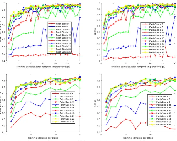
The impact of patch size from traditional LBP and SID_LBP is also needed to investigate. Take
Indian Pine dataset as an example, when we selected the first PCs as the source, the impact of
patch size on classification is shown in Fig.4.
As shown in Fig.4, it can be seen that the accuracy tends to be the maximum with
17 17
or larger. Therefore, we investigate the impact of the PCs’ number with the
17 17
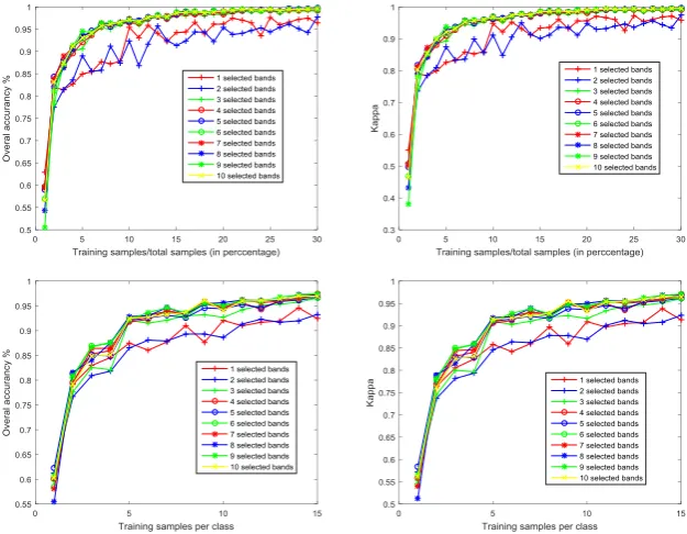
patch size.To investigate the effects of number of PCs for traditional LBP, the classification accuracy
[image:12.595.153.462.482.729.2]and time-consuming on patch size is
17 17
with different PCs number are shown in Fig.5,Table3.
Figure 4. Classification performance versus different patch sizes and different training samples
different patch sizes and different training samples selected same number training samples in different classes;
Figure 5. Classification performance versus different selected bands number and different training samples with the 17 17 patch size (a): Overal accuracy versus d different selected bands number and different training samples selected as ratio of training samples and total samples with the 17 17 patch size;(b) Kappa accuracy versus different selected bands number and different training samples selected as ratio
of training samples and total samples with the 17 17 patch size; (c) Overal accuracy versus different selected bands number and different training samples selected same number training samples in different classes with the 17 17 patch size;(d) Kappa accuracy versus different selected bands number and different training samples selected same number training samples in different classes with the 17 17 patch size;
Table 3 Time-consuming versus different selected bands number and different training samples
1 2 3 4 5 6 7 8 9 10
samples selected as ratio of training
samples and total samples 0.6167 0.9934 1.4711 1.8363 2.2492 2.7788 3.1375 3.5714 4.0166 4.4571
samples selected same number
training samples in different classes 0.9048 0.9983 1.3909 1.8908 2.2741 2.8497 3.0978 3.5740 4.0126 4.5305
From the Figures and Tables, we can see that the accuracy difference is not obvious above the
3 PCs. Note that the LBP features dimension and time-cost are dramatically increased with
selected bands number. Therefore, we employed the 3 PCs and
17 17
patch size for traditionalLBP.
C. Numerical Results
1) Classification of Indian Pines Image
In this set of experiments, we first evaluated the classification accuracy of the proposed
approach using the AVIRIS Indian Pines data set in Fig.2. Table 4 shows the OAs (in percent) in
traditional LBP and SID_LBP. In order to show the performance of our proposed approach under
Bands number Samples selection
[image:13.595.82.516.412.471.2]different training conditions and scenarios, in the second experiments, we choose same training
samples per class for classification assessment. Although the training samples are chosen
randomly, we chosen the same training samples for comparison between two methods.
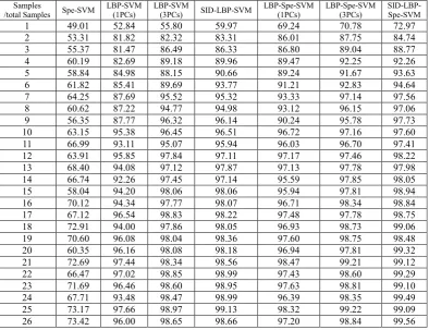
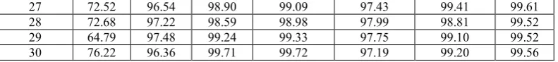
There are several conclusions can obtained from the Tables below. First of all, SID_LBP
method has much better performance than original spectral signatures only. For example, in Table
v, LBP-SVM (1PCs) offers 3.83% higher accuracy than the original spectrum classification in 1%
training samples and 16.18% in 5 samples chosen per class. With the training samples number
increase, LBP-SVM only use 1PCs offers over 20% higher accuracy than original spectrum
classification; LBP-SVM (3PCs) , SID_LBP-SVM, LBP-Spe-SVM (1PCs) , LBP-Spe-SVM
(3PCs) and SID-LBP-Spe-SVM offers 6.8%, 10.96%,20.23%, 21.77% and 23.96% higher
accuracy individually in 1% training samples.
Secondly, spectral-spatial feature classification exhibits the potential to improve the
classification results compared with using spectrum information and spatial information. For
example, LBP-Spe-SVM (1PCs), LBP-Spe-SVM (3PCs) and SID_LBP-Spe-SVM which joined
the spectrum and spatial information offers higher accuracy than Spe-SVM which is only using
spectrum information and LBP-SVM (1PCs), LBP -SVM (3PCs) and SID_LBP-SVM which are
only using spatial information.
Thirdly, the SID_LBP proposed exhibits the potential to improve the classification results
than using the traditional LBP. For example, SID_LBP–SVM offers over 7.07% higher accuracy
than LBP-SVM (1PCs) and 4.17% higher than LBP-SVM (3PCs) , and SID-LBP-Spe-SVM is
3.67% higher than LBP-Spe-SVM (1PCs) and 2.19% higher than LBP-Spe-SVM (3PCs) in 1%
0.24% higher than LBP-SVM (3PCs) , and SID-LBP-Spe-SVM is 2.98% higher than
LBP-Spe-SVM (1PCs) and 0.79% higher than LBP-Spe-SVM (3PCs) in 5 training samples per
class.
Furthermore, it is noticeable that SID_LBP is more effective than traditional LBP (1PCs) and
also can save more time than traditional LBP (3PCs). According to what we analyzed before, the
LBP (3PCs) will extract the texture feature three times than SID_LBP method while the texture
feature is done by calculating the histograms which is time-consuming.
Finally, it is observed that the obtained results which involved the spatial information are
much better than the spectral information alone. This demonstrates that LBP is a highly
discriminative spatial operator.
We also can get information that the SID_LBP method gets less and less effeteness with the
[image:15.595.102.497.467.770.2]samples number increases.
Table 4 Overal classifications accuracy (in percent) obtained for different classification methods when applied to the AVIRIS Indian Pines Hyperspectral data set using different percent training samples
Samples
/total Samples Spe-SVM LBP-SVM (1PCs) LBP-SVM (3PCs) SID-LBP-SVM LBP-Spe-SVM (1PCs) LBP-Spe-SVM (3PCs) SID-LBP- Spe-SVM
1 49.01 52.84 55.80 59.97 69.24 70.78 72.97
2 53.31 81.82 82.32 83.31 86.01 87.75 84.74
3 55.37 81.47 86.49 86.33 86.80 89.04 88.77
4 60.19 82.69 89.18 89.96 89.47 92.25 92.26
5 58.84 84.98 88.15 90.66 89.24 91.67 93.63
6 61.82 85.41 89.69 93.77 91.21 92.83 94.64
7 64.25 87.69 95.52 95.32 93.33 97.14 97.56
8 60.62 87.22 94.77 94.98 93.12 96.15 97.06
9 56.35 87.77 96.32 96.14 90.24 95.78 97.73
10 63.15 95.38 96.45 96.51 96.72 97.16 97.60
11 66.99 93.11 95.07 95.94 96.03 96.70 97.41
12 63.91 95.85 97.84 97.11 97.17 97.46 98.22
13 68.40 94.08 97.12 97.87 97.13 97.78 97.98
14 66.74 92.26 97.45 97.14 95.59 97.85 98.05
15 58.04 94.20 98.06 98.06 95.94 97.81 98.94
16 70.12 94.34 97.77 98.07 96.71 98.34 98.84
17 67.12 96.54 98.83 98.22 97.48 97.78 98.75
18 72.91 94.00 97.86 98.05 96.93 98.73 99.06
19 70.60 96.08 98.04 98.36 97.60 98.75 98.48
20 60.35 96.16 98.08 98.18 96.94 97.81 99.32
21 72.69 97.44 98.34 98.56 98.47 99.21 99.12
22 66.47 97.02 98.85 98.99 97.43 98.60 99.29
23 71.69 96.46 98.60 98.95 97.63 98.81 99.10
24 67.71 93.48 98.47 98.99 96.39 98.35 99.49
25 73.17 97.66 98.97 99.13 98.32 99.22 99.09
27 72.52 96.54 98.90 99.09 97.43 99.41 99.61
28 72.68 97.22 98.59 98.98 97.99 98.81 99.52
29 64.79 97.48 99.24 99.33 97.75 99.10 99.52
30 76.22 96.36 99.71 99.72 97.19 99.20 99.56
Table 5 Overal classifications accuracy (in percent) obtained for different classification methods when applied to the AVIRIS Indian Pines Hyperspectral data set using different percent training samples
Samples
Per class Spe-SVM LBP-SVM (1PCs) LBP-SVM (3PCs) SID-LBP-SVM LBP-Spe-SVM (1PCs) LBP-SVM (3PCs) SID-LBP- Spe-SVM
5 43.73 59.70 59.90 60.14 68.95 71.14 71.93
10 46.97 79.17 79.66 79.92 83.59 85.47 84.71
15 52.08 82.96 82.56 82.61 86.90 88.39 87.41
20 53.73 84.59 82.11 84.81 89.56 88.86 90.84
25 57.71 87.48 92.07 87.32 92.89 95.85 92.45
30 59.03 86.06 91.51 85.47 88.50 95.26 88.55
35 55.39 87.71 92.12 89.18 90.14 94.91 91.71
40 62.37 90.98 92.97 91.76 94.13 95.37 94.57
45 58.54 87.64 93.24 93.99 92.52 95.43 96.00
50 61.60 92.07 92.68 92.69 95.15 95.68 94.89
55 61.73 90.98 94.19 94.31 93.94 96.68 96.34
60 63.56 91.69 95.12 93.05 94.27 96.85 95.40
65 61.85 91.94 95.32 93.26 94.23 96.76 95.37
70 61.38 94.61 95.76 95.88 96.37 97.64 97.52
75 64.19 92.43 96.57 96.32 95.16 97.99 97.91
2) Classification of University of Pavia Image
In this set of experiments, we first evaluated the classification accuracy of the proposed
approach using the ROSIS university of Pavia data set in Fig.3. Table 6 shows the OAs (in percent)
in traditional LBP and SID_LBP. In order to show the performance of our proposed approach
under different training conditions and scenarios, in the second experiments, we choose same
training samples per class for classification assessment.
There are several conclusions can be obtained from the Tables below. First of all, With the
LBP features, the performances are much better than with the original spectral signatures only; for
example, in Table 6, LBP-SVM (1PCs) offers 3.94% high accuracy than the original spectrum
classification in 1% training samples and 13.81% in 5 samples chosen per class. With the training
samples number increase, LBP-SVM which only use 1PCs offers over 20% high accuracy than
original spectrum classification; LBP-SVM (3PCs) , SID_LBP-SVM, LBP-Spe-SVM (1PCs) ,
LBP-Spe-SVM (3PCs) and SID-LBP-Spe-SVM offers 4.99%, 9.94%,16.95%, 18.70% and
23.80% high accuracy individually than the original spectrum classification in 1% training
[image:16.595.102.498.73.117.2]Secondly, spectral-spatial feature classification exhibits the potential to improve the
classification results than only using spectrum information and spatial information. For example,
LBP-Spe-SVM (1PCs), LBP-Spe-SVM (3PCs) and SID_LBP-Spe-SVM that join the spectrum
and spatial information offers higher accuracy than Spe-SVM only using spectrum information
and LBP-SVM (1PCs), LBP -SVM (3PCs) and SID_LBP-SVM only using spatial information.
Thirdly, the SID_LBP proposed exhibits the potential to improve the classification results
than using the traditional LBP. For example, SID_LBP–SVM offers over 5% higher accuracy than
LBP-SVM (1PCs) and 4.95% higher than LBP-SVM (3PCs) , and SID-LBP-Spe-SVM is 6.85%
higher than LBP-Spe-SVM (1PCs) and 6.10% higher than LBP-Spe-SVM (3PCs) in 1% training
samples; SID_LBP–SVM offers over 1.73% higher accuracy than LBP-SVM (1PCs) and 0.49%
higher than LBP-SVM (3PCs) , and SID-LBP-Spe-SVM is 3.26% higher than LBP-Spe-SVM
(1PCs) and 0.48% higher than LBP-Spe-SVM (3PCs) in 5 training samples per class.
Furthermore, it is noticeable that SID_LBP is more effective than traditional LBP (1PCs) and
time-saving than traditional LBP (3PCs). Accordance to what we analyzed before, the LBP (3PCs)
will extract the texture feature three times than SID_LBP method while the texture feature is done
by calculating the histograms which is time-consuming.
Finally, it is observed that the obtained results involving the spatial information are much
better than the spectral information alone. This demonstrates that LBP is highly discriminative
spatial operator.
We also can get information that the SID_LBP method gets less and less effeteness with the
samples number increases.
Table 6 Overal classifications accuracy (in percent) obtained for different classification methods when applied to the AVIRIS Indian Pines Hyperspectral data set using different percent training samples
Samples
1 51.29 55.23 56.28 61.23 68.24 69.99 75.09
2 56.44 71.82 79.72 84.12 88.01 87.75 88.09
3 58.72 79.57 83.66 87.22 85.12 89.04 89.97
4 61.65 82.78 83.12 91.02 89.44 92.12 92.96
5 62.64 83.67 89.65 89.11 87.22 91.37 93.12
6 63.55 85.52 88.22 92.66 89.17 92.35 94.57
7 65.27 86.99 93.12 93.12 93.01 97.42 97.99
8 62.11 87.75 94.99 95.12 93.19 96.67 97.62
9 60.96 88.93 95.17 96.56 95.24 95.12 97.07
10 62.25 91.28 96.37 95.49 93.72 97.56 97.99
11 66.99 93.58 95.33 95.37 93.03 96.99 97.91
12 63.91 92.66 95.84 97.29 96.11 97.02 98.56
13 65.92 95.18 96.12 97.22 97.09 97.29 98.98
14 67.29 93.45 97.41 98.23 94.29 97.69 98.92
15 66.09 94.02 97.02 98.01 95.74 97.99 98.99
16 70.25 94.12 96.01 98.59 95.71 98.96 99.02
17 70.09 95.99 97.12 98.23 96.48 97.02 98.99
18 71.11 94.09 96.11 98.33 95.12 98.58 99.36
19 72.99 96.22 98.31 98.45 97.69 98.65 98.96
20 70.01 96.34 98.39 98.61 96.48 97.41 98.93
21 73.67 97.42 98.54 98.72 98.11 98.12 99.36
22 70.28 97.83 98.55 98.67 96.21 98.23 99.69
23 78.99 96.16 98.12 98.23 97.09 98.71 99.90
24 76.38 93.38 98.22 98.99 95.29 98.61 99.59
25 75.29 97.35 98.23 99.45 97.32 99.01 99.49
26 76.29 96.28 98.23 98.79 97.98 98.45 99.66
27 77.79 96.17 98.88 99.66 97.64 99.66 99.69
28 77.89 97.96 98.56 98.23 97.27 98.21 99.52
29 78.25 97.21 99.12 99.33 97.59 99.39 99.59
30 78.99 96.09 99.11 99.79 97.74 99.45 99.69
Table 7 Overal classifications accuracy (in percent) obtained for different classification methods when applied to the AVIRIS Indian Pines Hyperspectral data set using different percent training samples
Samples
Per class Spe-SVM LBP-SVM (1PCs) LBP-SVM (3PCs) SID-LBP-SVM LBP-Spe-SVM (1PCs) LBP-SVM (3PCs) SID-LBP- Spe-SVM
5 49.01 62.84 64.08 64.57 69.51 72.69 73.17
10 53.31 81.82 79.32 87.81 70.12 87.28 89.11
15 55.37 81.47 86.49 90.29 71.41 88.96 89.58
20 60.19 82.69 89.18 94.07 70.44 88.75 90.96
25 58.84 84.98 88.15 93.34 71.92 93.21 93.49
30 61.82 85.41 89.69 95.26 71.01 95.16 95.55
35 64.25 87.69 94.52 96.09 72.82 93.91 94.12
40 60.62 87.22 93.77 b96.87 71.21 95.12 95.21
45 56.35 87.77 94.32 96.89 71.91 95.99 96.65
50 63.15 95.38 96.45 97.22 72.47 95.46 95.47
55 66.99 93.11 95.07 98.18 72.93 96.92 96.99
60 63.91 95.85 95.84 97.68 74.08 95.72 95.72
65 68.40 94.08 95.12 95.18 73.28 95.48 95.37
70 66.74 92.26 95.45 97.98 73.84 97.69 97.99
75 68.04 94.20 97.06 97.16 74.21 97.76 98.01
5. Conclusion and Future research Lines
In this paper, we have developed a new texture feature extraction algorithm exploits spatial
texture feature from spectrum. The method is proposed by employing local binary patterns (LBPs)
to extract the image texture with respect to spectrum information diversity (SID) to measure the
differences of spectrum information. Compared with the traditional LBP with the same classifier,
foremost, The performances with SID_LBP are much better than with the original spectral
signatures only, which demonstrates that the LBP is a highly discriminative spatial operator;
Second, spectral-spatial joint feature is doing well than spectrum only and spatial feature only,
which means spatial information is also important for spectral image classification; Third,
SID_LBP is more effective than traditional LBP (1PCs) and time-saving than traditional LBP
(3PCs) while the performance between them is almost the same; Finally, SID_LBP method gets
less and less effeteness with the samples number increases, because that the more samples
provides more spatial information than spectrum aspect.
Although the results obtained are very encouraging, further experiments with additional
scenes and comparison methods should be conducted. We also need to choose some other
classifiers for experiments.
Acknowledgments
This work was supported in part by National Natural Science foundations of China (Grant
Nos. 41301382, 61401439, 41604113, 41711530128) and foundation of Key lab of spectral
imaging, Xi’an Institute of Optics and Precision Mechanics of CAS.
References
1 Richards, John A. Remote Sensing Digital Image Analysis. Remote sensing digital image
analysis :. Springer-Verlag, 1986:47-54.
2 Bandos, Tatyana V., L. Bruzzone, and G. Camps-Valls. "Classification of Hyperspectral Images
With Regularized Linear Discriminant Analysis." IEEE Transactions on Geoscience & Remote
Sensing 47.3(2009):862-873.
3 Li, Wei, et al. "Locality-Preserving Dimensionality Reduction and Classification for
50.4(2012):1185-1198.
4 Ma, Li, M. M. Crawford, and J. Tian. "Local Manifold Learning-Based, -Nearest-Neighbor for
Hyperspectral Image Classification." Geoscience & Remote Sensing IEEE Transactions on
48.11(2010):4099-4109.
5 Zenzo, Silvano Di, et al. "Gaussian Maximum Likelihood and Contextual Classification
Algorithms for Multicrop Classification." IEEE Transactions on Geoscience & Remote Sensing
GE-25.6(1987):815-824.
6 Stathakis, D., and A. Vasilakos. "Comparison of computational intelligence based classification
techniques for remotely sensed optical image classification." Geoscience & Remote Sensing IEEE
Transactions on 44.8(2006):2305-2318.
7 Tuia, Devis, et al. "Learning Relevant Image Features With Multiple-Kernel Classification."
IEEE Transactions on Geoscience & Remote Sensing 48.10(2010):3780-3791.
8 Bandos, Tatyana V., L. Bruzzone, and G. Camps-Valls. "Classification of Hyperspectral Images
With Regularized Linear Discriminant Analysis."IEEE Transactions on Geoscience & Remote
Sensing 47.3(2009):862-873.
9 Gu, Yanfeng, et al. "Representative Multiple Kernel Learning for Classification in
Hyperspectral Imagery." IEEE Transactions on Geoscience & Remote Sensing
50.7(2012):2852-2865.
10 Li, Jun, et al. "Generalized Composite Kernel Framework for Hyperspectral Image
Classification." IEEE Transactions on Geoscience & Remote Sensing 51.9(2013):4816-4829.
11 Camps-Valls, G., et al. "Composite kernels for hyperspectral image classification." IEEE
Geoscience & Remote Sensing Letters3.1(2006):93-97.
12 Benediktsson, J. A., J. A. Palmason, and J. R. Sveinsson. "Classification of hyperspectral data
from urban areas based on extended morphological profiles." IEEE Transactions on Geoscience &
Remote Sensing 43.3(2005):480-491.
13 Mura, Mauro Dalla, et al. "Extended profiles with morphological attribute filters for the
analysis of hyperspectral data." International Journal of Remote Sensing 31.22(2010):5975-5991.
samples using CLBP." Proceedings(1945):1011-1014.
15 Li, Wei, et al. "Local Binary Patterns and Extreme Learning Machine for Hyperspectral
Imagery Classification." IEEE Transactions on Geoscience & Remote Sensing 53.7(2015):1-13.
16 Huang, Xin, and L. Zhang. "An SVM Ensemble Approach Combining Spectral, Structural, and
Semantic Features for the Classification of High-Resolution Remotely Sensed Imagery." IEEE
Transactions on Geoscience & Remote Sensing 51.1(2013):257-272.
17 Chen, Chen, et al. "Spectral–Spatial Preprocessing Using Multihypothesis Prediction for
Noise-Robust Hyperspectral Image Classification." IEEE Journal of Selected Topics in Applied
Earth Observations & Remote Sensing 7.4(2014):1047-1059.
18 Gong, Yunchao, and S. Lazebnik. "Iterative quantization: A procrustean approach to learning
binary codes." IEEE Conference on Computer Vision and Pattern Recognition. IEEE Computer
Society, 2011:817-824.
19 Guo, Yuchen, et al. "Learning to Hash with Optimized Anchor Embedding for Scalable
Retrieval." IEEE Transactions on Image Processing.PP. 99(2017):1-1.
20 Lin Z, et al. "Cross-View Retrieval via Probability-Based Semantics-Preserving Hashing."
IEEE Transactions on Cybernetics.PP.99(2016):1-14.
21 Guo, Yuchen, et al. "Zero-Shot Learning With Transferred Samples." IEEE Transactions on
Image Processing 26.7(2017):3277-3290.
22 Doshi, N. P., G. Schaefer, and S. Y. Zhu. "An Evaluation of LBP Texture Descriptors for the
Classification of HEp-2 Cells." IEEE International Conference on Systems, Man, and Cybernetics
IEEE, 2015.
23Kumar, V. Vijaya, K. S. Reddy, and V. V. Krishna. "Face recognition using prominent LBP
model." International Journal of Applied Engineering Research 10.2(2015):4373-4384.
24Ojala, Timo, M. Pietikäinen, and T. Mäenpää. "Multiresolution Gray-Scale and Rotation
Invariant Texture Classification with Local Binary Patterns." IEEE Transactions on Pattern
Analysis & Machine Intelligence 24.7(2002):971-987.
support vector machines." IEEE Transactions on Geoscience & Remote Sensing
42.8(2004):1778-1790.
26 Chang, Chein I. "An information-theoretic approach to spectral variability, similarity, and
discrimination for hyperspectral image analysis." IEEE Transactions on Information Theory