Grassmann Learning for Recognition and Classification

(1)

Rochester Institute of Technology

RIT Scholar Works

Theses Thesis/Dissertation Collections

1-1-2014

Grassmann Learning for Recognition and

Classification

Sherif Azary

Follow this and additional works at:http://scholarworks.rit.edu/theses

This Dissertation is brought to you for free and open access by the Thesis/Dissertation Collections at RIT Scholar Works. It has been accepted for inclusion in Theses by an authorized administrator of RIT Scholar Works. For more information, please [email protected]. Recommended Citation

(2)

Grassmann Learning for Recognition and

Classification

Ph.D. Dissertation by Sherif Azary

B. THOMAS GOLISANO COLLEGE OF COMPUTING AND INFORMATION SCIENCES

DEPARTMENT OF COMPUTING AND INFORMATION SCIENCES-PHD

ROCHESTER INSTITUTE OF TECHNOLOGY

ROCHESTER, NEW YORK

Date:

Monday, April 28, 2014

Dissertation Advisor:

Dr. Andreas Savakis, Professor, Department of Computer Engineering, RIT

Dissertation Committee:

Dr. Nathan D. Cahill, Associate Professor, School of Mathematical Sciences, RIT

Dr. Shanchieh J. Yang, Associate Professor & Department Head, Department of Computer Engineering, RIT Dr. Richard Zanibbi, Associate Professor, Department of Computer Science, RIT

Defense Chair:

(3)

i

B. THOMAS GOLISANO COLLEGE OF

COMPUTING AND INFORMATION SCIENCES

ROCHESTER INSTITUTE OF TECHNOLOGY

ROCHESTER, NEW YORK

CERTIFICATE OF APPROVAL

The Ph.D. Degree Dissertation of Sherif Azary has been examined and approved by the

dissertation committee as complete and satisfactory for the dissertation requirement for Ph.D.

degree in Computing and Information Sciences

____________________________________

Dr. Andreas Savakis, Advisor (date)

____________________________________

Dr. Nathan D. Cahill, Member (date)

____________________________________

Dr. Shanchieh J. Yang, Member (date)

____________________________________

Dr. Richard Zanibbi, Member (date)

____________________________________

Dr. Dhireesha Kudithipudi, Defense Chair (date)

_________________________________________________

Dr. Pengcheng Shi, Ph.D. Program Director (date)

(4)

ii

Abstract

Computational performance associated with high-dimensional data is a common challenge

for real-world classification and recognition systems. Subspace learning has received

considerable attention as a means of finding an efficient low-dimensional representation that

leads to better classification and efficient processing. A Grassmann manifold is a space that

promotes smooth surfaces, where points represent subspaces and the relationship between points

is defined by a mapping of an orthogonal matrix. Grassmann learning involves embedding high

dimensional subspaces and kernelizing the embedding onto a projection space where distance

computations can be effectively performed.

In this dissertation, Grassmann learning and its benefits towards action classification and

face recognition in terms of accuracy and performance are investigated and evaluated.

Grassmannian Sparse Representation (GSR) and Grassmannian Spectral Regression (GRASP)

are proposed as Grassmann inspired subspace learning algorithms. GSR is a novel subspace

learning algorithm that combines the benefits of Grassmann manifolds with sparse

representations using least squares loss ℓ1_{-norm minimization for improved classification.}

GRASP is a novel subspace learning algorithm that leverages the benefits of Grassmann

manifolds and Spectral Regression in a framework that supports high discrimination between

classes and achieves computational benefits by using manifold modeling and avoiding

eigen-decomposition. The effectiveness of GSR and GRASP is demonstrated for computationally

intensive classification problems: (a) multi-view action classification using the IXMAS

Multi-View dataset, the i3DPost Multi-Multi-View dataset, and the WVU Multi-Multi-View dataset, (b) 3D action

(5)

iii

recognition using the ATT Face Database, Labeled Faces in the Wild (LFW), and the Extended

Yale Face Database B (YALE).

Additional contributions include the definition of Motion History Surfaces (MHS) and

Motion Depth Surfaces (MDS) as descriptors suitable for activity representations in video

sequences and 3D depth sequences. An in-depth analysis of Grassmann metrics is applied on

high dimensional data with different levels of noise and data distributions which reveals that

standardized Grassmann kernels are favorable over geodesic metrics on a Grassmann manifold.

Finally, an extensive performance analysis is made that supports Grassmann subspace learning

(6)

iv

Acknowledgements

I would like to express my deepest gratitude to my advisor, Dr. Andreas Savakis, for his

guidance, support, patience, mentorship, and encouragement in making this research possible.

Dr. Andreas Savakis has always been accommodating to my schedule and encouraged me to

complete my research while I worked full-time and moved away from Rochester, NY to further

my career. Without this encouragement I would not be where I am today and I am grateful. Dr.

Andreas Savakis and Dr. Shanchieh J. Yang have also provided financial support for my PhD

research and I thank them for believing in me.

I would also like to thank my committee and defense chair, Dr. Nathan D. Cahill, Dr.

Shanchieh J. Yang, Dr. Richard Zanibbi, and Dr. Dhireesha Kudithipudi for their support and

advice in making this dissertation possible. They have always been accommodating to my

schedule and extremely supportive to make this research productive and stimulating. It has been

an honor. I would like to thank Dr. Pengcheng Shi for accepting me into the Computing and

Information Science Ph.D. program and believing in me to complete my research as a part-time

student with a full-time job.

I would like to thank my colleagues, Dr. Grigorios Tsagkatakis and Dr. Raymond Ptucha,

for their friendship, academic advice, and words of encouragement. I also cannot express

enough appreciation to Joyce Hart, Kathryn Stefanik, and Lorrie Jo Turner for their academic

support.

I would like to thank my brother and his wife, Hani and Mary Azary, for their continuous

words of encouragement and being great friends. I would like to thank my brother in law,

Johnny Girgis, and my good friend, Pete Henen, for their friendship and humor. I would like to

thank my parents, Wahid and Samia Azary, for their patience, love, and raising me with a

passion for problem solving and math. I owe the success of my education and my career to

them. Finally, I would like to thank my wife, May, for always being there for me, and for her

(7)

v

1 Introduction

The automatic recognition of human actions a fundamental but challenging task in computer

vision research for a wide variety of applications including autonomous surveillance, law

enforcement, health care monitoring systems, and human computer interfacing. Automatic face

recognition is another important task for many applications. The main challenge of such systems

is their ability to classify in unconstrained environments. Images of human actors can vary by

their sizes, shapes, poses, occlusions, viewpoint variations, noise, and lighting. Additionally,

action classification systems would need to account for action execution speed requiring

spatio-temporal representations that are invariant to such factors.

The most common approaches to classification involve extracting meaningful features from

images or video and applying statistical or machine learning tools to make classification

decisions. Optimal action representations are those that can capture both the spatial structure of

an activity and its temporal structure over time. While many features can represent spatial and

temporal domains independently, there are spatio-temporal features that are capable of

representing both domains, such as space-time interest points and 3D Harris corner detectors.

Such features are well-suited for challenging applications such as multi-view and 3D action

classification systems. Within these domains are a wide variety of representations involving

normalization, invariance, and exhaustive search. Similarly, face image representations are

expected to be robust enough to distinguish between a wide range of human subjects and under

unconstrained conditions such as variations in illumination and facial expressions. Local binary

patterns and local ternary patterns are among the most popular face image representations.

Methodologies that can account for the statistical and geometric properties of high

(11)

2 | P a g e information. Principal component analysis (PCA) is a common dimensionality reduction method

based on the eigenvectors of the covariance matrix. Although fast, PCA does not maintain

geometry and local structuring of high dimensional data. Manifold learning techniques have

been developed to handle non-linear dimensionality reduction. Manifold learning involves

reducing high dimensional data to a lower dimensional space while optimally preserving the

local geometries from the high dimensional information. An ideal mapping should be fast,

preserve clustering, and account for occlusions and outliers. There are many dimensionality

reduction algorithms that are powerful enablers of robust classification and in this dissertation

the benefits and drawbacks of many of these methods are discussed. As an alternative, sparse

representations are methods of finding sparse solutions that are useful in a variety of applications

including classification.

Grassmann learning is a dimensionality reduction algorithm where subspaces are mapped as

points onto a smooth and curved surface where distances between subspaces are geodesic. The

main advantage of Grassmann learning over traditional manifold learning methods is that high

dimensional feature representations may not typically lie on a Euclidean space. Grassmann

learning maps subspaces onto points based on orthogonal constraints, promoting high

between-class discrimination by their geometrical structuring, and accounting for missing data through

subspace spanning. Grassmann kernelization embeds subspaces onto a projection space where

distance computations can be effectively performed.

In this dissertation, representations for action classification and face recognition systems are

explored in Chapter 2. Spatio-temporal surface descriptors for multi-view and 3D action

classification systems are presented using radial distance measures and 3D joint descriptors for

(12)

3 | P a g e representing actions while being invariant to time, scale, and localization. These spatio-temporal

surface representations motivated the development of more robust motion surface

representations. Motion surfaces, proposed in this dissertation, have proven to be very effective

representations for describing where motion exists in a scene and how motion evolves over time.

Motion history surface (MHS) and motion depth surface (MDS) descriptors are suitable for

activity representations for multi-view and 3D depth action sequences.

In Chapter 3 dimensionality reduction algorithms including principal component analysis,

multidimensional scaling, local linear embedding, and linear extensions of graph embedding are

discussed and evaluated. The benefits and drawbacks of these methods are identified including

time complexities. Grassmann learning and its benefits towards action classification and face

recognition in terms of accuracy and performance are investigated in Chapter 4. Grassmann

learning in a kernelized principal component analysis framework is defined and evaluated. In

Chapter 5, Grassmannian Sparse Representation (GSR) is proposed as a Grassmann inspired

subspace learning algorithm. GSR is a novel subspace learning algorithm that combines the

benefits of Grassmann manifolds with sparse representations using least squares loss ℓ1-norm

minimization for improved classification. Sparse representations are introduced as a method for

finding sparse solutions for underdetermined systems. Images and video sequences can be

encoded using sparse representations to be more easily interpretable and classification using least

squares loss ℓ1_{-norm minimization shows to be suitable for classification at the cost of poor}

computational performance. This framework is extended into a Grassmann learning framework

through GSR. The high cost of poor performance through GSR encouraged the pursuit of a

faster learning framework. Grassmannian Spectral Regression (GRASP) is introduced in

(13)

4 | P a g e Grassmann manifolds and Spectral Regression in a framework that supports high discrimination

between classes and achieves computational benefits by using manifold modeling and avoiding

eigen-decomposition.

In Chapter 7, the classification accuracies and performance of all previously discussed

learning methods including GSR and GRASP are presented for computationally intensive action

and face datasets. An in-depth analysis of Grassmann metrics is applied on high dimensional

data with different levels of noise and data distributions revealing that standardized Grassmann

kernels are favorable over Grassmann geodesic metrics in a Grassmann space. GSR and GRASP

are compared against existing sparse representations, manifold learning, and Grassmann learning

methodologies. An extensive performance analysis is made that support Grassmann subspace

learning through GSR and GRASP as effective approaches for classification and recognition

over state-of-the-art approaches. The dissertation concludes in Chapter Error! Reference

source not found..

1.1 Contributions

In this section the contributions made in this dissertation are explicitly defined. The first is the

definition of radial distances and radial distance surfaces as action representations. Such

surfaces have shown to be suitable representations for multi-view action classification. This

work was extended to handle 3D action sequences using 3D joint surface descriptors. This led to

the evolution of motion surfaces where motion history surfaces (MHS) and motion depth

surfaces (MDS) are proposed as descriptors that can accurately represent motion in multi-view

(14)

5 | P a g e The main contributions of this dissertation are the definition of Grassmannian Sparse

Representations and Grassmannian Spectral Regression for high classification accuracy and

computational performance. With this, an extensive evaluation is made on Grassmann metrics

which is not found at this level of depth in the existing literature. Through experiments and

evaluation, this dissertation exposes the benefit of using Grassmann kernels with robust

classifiers over geodesic metrics using kernel standardization. Additionally, a thorough time

(15)

6 | P a g e

2 Representations for Action Classification and Face Recognition

2.1 Action Representations

Weinland et al. [1] discuss a broad range of spatial, temporal, and spatio-temporal approaches for

addressing action classification problems. Spatial action representations attempt to describe the

spatial structure of actions. Body models [2], body pose estimations [3], kinematic joint models

[4], and stick figures [5] tend to be intuitive and descriptive, but may require significant training

and computational resources. Spatial parametric image features include contour/silhouette

representations [6], optical flow [7], and motion history images/motion energy images [8]. Such

features do not require body part labeling or tracking, but are computationally intensive because

of high dimensional data representations and difficulties with occlusions. Spatial statistical

approaches are based on the statistics of local features, such as features detected using the Harris

corner detector [9]. Local feature descriptors can be classified using Bag of Features [10],

Support Vector Machines (SVM’s) [11], local Principal Component Analysis (local PCA) [12],

and Manifold Learning - e.g. supervised locality preserving projections (sLPP) [13]. The main

benefits of spatial statistical representations are that they are not relying on body part labeling,

silhouette extraction, and localization. However, such representations are usually unordered and

of varying sizes making it difficult to use with classifiers.

Temporal representations of human actions identify the temporal structure of an action and

are categorized into action grammars [14], action templates [15], and temporal statistics [16].

Action grammars identify an action by a set of action primitives. Given a set of all action

primitives, an action grammar acts as a function to learn the transitions between those primitives.

A popular method for identifying action primitive transitions is the use of Hidden Markov

(16)

7 | P a g e including Kruger and Grest [17] and Chakraborty et al. [18]. Action grammars are highly

modular but require manual structuring making action grammars impractical for systems

intended to classify a large set of action classes. Action templates are a combination of action

primitives into one larger representation. Pattern matching is usually applied to compare actions

to a collection of action templates in a database. Junejo et al. [19] propose a view independent

approach to action recognition on 2D video sequences using Self Similarity Matrices (SSM).

Their approach captures temporal histograms of gradient orientations in the spatial domain and

concatenates the features descriptors into one large local SSM feature vector descriptor. This

feature vector descriptor is an action template. Yao et al. [20] collect action pose templates as a

combination of Histogram of Gradient (HoG) features and Histogram of Optical Flow (HoF)

features. These templates are classified using Support Vector Machines (SVM’s). Action

templates are known to be effective and discriminative, but do not have a built-in mechanism to

account for temporal segmentation. Temporal statistics find statistical patterns of actions in the

temporal domain such as identifying frequent features over time.

Spatio-temporal representations are those that can describe an action structure in both the

spatial and temporal domains. One of the earliest spatio-temporal feature descriptors was

introduced by Laptev and Lindeberg [21] by extending on the Harris Corner Detector algorithm

to detect space-time interest points that can be used to represent motion-based activities. Other

spatio-temporal interest points include cuboids using temporal Gabor filters [22], Harris 3D

detectors as a 3D extension of the Harris corner detector for detecting significant local variations

on both space and time [23], and Hessian detectors that are scale and affine invariant across the

space and time domains [24]. Vili et al. [25] introduce dynamic texture descriptors to describe

(17)

8 | P a g e Patterns are used to extract histogram features in the XT and YT spaces. An interesting action

representation that inspired the action descriptor used in this dissertation is the spatio-temporal

action surfaces covered by Souvenir and Parrigan [26]. The 2D Radon transform was applied on

each frame of an action and converted to a 1D signal called the R-Transform. A surface was

created as a sequence of these signals called the RXS surface. These surfaces are then scaled

down to a standard time interval while preserving action information supporting the concept of

spatio-temporal invariance.

2.1.1 Action Representations for Multi-View and 3D Applications

Autonomous action classification systems can be restricted by visual sensor constraints or benefit

from their physical positions in a scene. Multiple view recognition systems tend to use standard

RGB cameras, while 3D cameras used in the gaming industry can provide both color and depth

information. An overview of multi-view and 3D action classification systems are discussed in

this section.

Weinland et al. [1] explain that viewpoint independence is commonly addressed by

normalization, invariance, or exhaustive search. View normalization is based on correcting the

current view through a transformation to a canonical view. This approach is taken in the work of

Gkalelis et al. [27] who use multi-view posture vectors of synchronized frames along with a

combination of circular shifting Discrete Fourier Transforms to determine the posture of an

individual relative to the current view. Ding et al. [28] present a pose-normalization algorithm

using random forest embedded active shape models to map 2D features into a 3D corresponding

space. Similarly, Iosifidis et al. [29] applied morphological operations on binary body masks of

(18)

9 | P a g e along with centroid movements the relative posture of the body with respect to the current view.

Drawbacks of this approach are the scale and body shape dependency of the torsos as well as

expected physical translation across a scene to calculate the posture position. Iosifidis et al.’s

[30] later work approached the issues of torso and translation dependencies by creating multiple

view binary masks. Bodor et al. [31] used image based rendering to reconstruct views that

would be suitable for classifiers. Silhouettes from multiple cameras were captured and projected

into a 3D space so that the 3D motion path could be determined. These motion paths were then

used to determine the orthogonal views needed for classifiers. However, this system assumes

linear motion paths, so activities such as turning around and punching are not expected to be

easily classified.

A view-invariant matching approach depends on finding common features across multiple

views. Popular view-invariant feature representations are Self-Similarity Matrices (SSM) [19],

which represent distances between action representations, and Cross Ratios (CR) [32] which

determine common interest points across multiple action frames. View normalization methods

are based on a single transformation for body orientation and view invariance. In comparison,

SSM and CR methods, which ignore transformation dependent features, also perform an

exhaustive search over all possible transformations to identify matching pairs. These methods

are categorized as view-invariant and exhaustive. Holte et al. [33] propose view-invariant 3D

feature descriptors based on motion information which are the 3D Motion Context (3D-MC) and

the Harmonic Motion Context (HMC). Motion vectors computed from 2D action sequences are

extended to 3D flow using pixel to vertex correspondences which are combined to create 3D

motion vector fields. A combination of 3D-MC, which is a 3D extension of general shape

(19)

10 | P a g e are used to provide a view-invariant representation of an action. Normalized correlation

coefficients between the test and training action sequences are used to classify actions.

The recent availability of cost-effective depth cameras, such as the Microsoft Kinect sensor,

provides a significant advantage, as depth images can facilitate body posture estimation and

action classification. Benefits over traditional image sensors include automatic background

segmentation, limb identification and invariance to illumination, color, and texture. Shotton et

al. [34] used depth data to calculate kinematic joint positions using spatial mode distributions

along with randomized decision forests. Their approach is invariant to pose, body shape, and

clothing. Similarly Schwarz et al. [35] used depth cameras to identify points on a human with a

maximal geodesic distance from the body center of mass, along with optical flow to make

predictions on joint tracking while considering occlusions. Beyond kinematic joint tracking,

recent research has extended to understanding gestures and actions from depth maps using action

graphs [36], statistical analysis on actionlets [37], and Hidden Markov Models [38] [39].

2.2 Face Representations

Face image representations are encodings that describe facial images and, ideally, should be

robust enough to distinguish between human subjects. Eigenfaces [40] is an approach based on

finding principal components of face images that linearly project the image space to a low

dimensional feature space. Although effective under ideal lighting conditions, frontal pose and

neutral facial expressions, eigenfaces are not robust and outliers from varying lighting

conditions, view angles, and expressions can result in undesired classification errors. Fisherfaces

(20)

11 | P a g e being less sensitive to lighting and expressions. Laplacianfaces [42] preserve the local structure

of the image space and detects the face manifold structure.

A challenge for Eigenfaces, Fisherfaces, and Laplacianfaces is robustness to lighting

conditions and facial expressions. Tann and Triggs [43] identify three categories for dealing

with these factors which are appearance-based, normalization-based, and feature-based methods.

Appearance-based methods require building a large training set that covers varying illumination

conditions and expressions. Normalization-based methods involve the normalization techniques

such as histograms. This included gamma correction, Difference of Gaussian (DoG) Filtering,

and contrast equalization. Figure 2-3 shows eight different subjects under varying illumination

conditions and their corresponding normalization in the second row. The illumination invariant

approach illustrated was proposed by Tann and Triggs [43] using gamma corrections, DoG

filtering, masking, and contrast equalization.

Feature-based methods identify illumination and expression invariant features. One such

example is Local Binary Patterns (LBP) which has proven to be effective for texture

representations while being highly discriminative and invariant to global gray-level

transformations for lighting invariance. LBP is based on thresholding image pixel

neighborhoods and encoding a binary pattern. The original LBP method applies an operator on

each pixel of an image which thresholds the neighboring pixels at the value of the central pixel.

The result of this operator is an image patch with an 8-bit code. An example of a basic LBP

operator and its resulting 8-bit code is shown in Figure 2-1. The central pixel with value 77 is

analyzed with a 3x3 window. Any neighboring pixel values greater than 77 are assigned a

binary value of 1. Any that are less than 77 are assigned a binary value of 0. After applying the

(21)

12 | P a g e around the central pixel. The encoding is considered uniform if there is at most one transition

from 0 to 1 or 1 to 0 (i.e.: 1110001). The resulting encoding in the example provided is not

uniform because there are two transitions for 0 to 1 and 1 to 0. The uniform properties of image

patches are useful for histograms that identify uniform and non-uniform patterns.

Figure 2-1: The LBP operation and the resulting 8-bit encoding of the central pixel [43].

LBP is popular for face image representations [44] [45] and there are many extensions.

Ojala et al. [46] propose a scale and rotation invariant extension of LBP. The work in [47]

proposes patch-based descriptors using three-patch and four-patch binary patterns. The main

disadvantage of LPB’s is the lack of sensitivity to noise. Local Ternary Patterns [43] is an

extension of LBP that accounts for robustness to noise and weak illumination gradients by using

a three valued code instead of a binary code. Values within a certain tolerance are assigned a

value of 0, values above the tolerance are assigned a value of 1, and values below the tolerance

are assigned a value of -1. LTP encodings are demonstrated in the Figure 2-2. Figure 2-3

illustrates sample face images from the YALE database which have been illumination

normalized. The third and fourth rows show the result LBP and LTP images for those

(22)

[image:22.612.77.535.220.469.2]

13 | P a g e Figure 2-2: The LTP operation and the resulting 8-bit encoding of the central pixel [43].

Figure 2-3: Normalization based processing of face images from the YALE face database under different lighting conditions. The top row shows the original images and the second row shows the resulting illumination normalized face images. The third row shows the LBP image representations. The fourth row shows the LTP image representations.

2.3 Radial Distance Representations for Action Recognition

The first contribution in this dissertation is the definition of radial distance surfaces [13] as

efficient feature representations. Locality Preserving Projection (LPP), a manifold learning

technique, was used for learning low dimensional representations of action primitives to

(23)

14 | P a g e depth maps, 3D joint descriptors [48] are also proposed. Radial distances, radial distance

surfaces, 3D joint surfaces, and the manifold learning framework are presented in this section.

2.3.1 Radial Distance Measures

Radial distances are features based on distances from a centroid to the outer contour of a

silhouette. A manifold learning framework was used for obtaining low dimensional

representations of action primitives that can be used to recognize activities across multiple views.

For each frame of an entire activity video, silhouettes were represented by binary images after

background subtraction. To efficiently describe a silhouette in some detail while maintaining

robustness to noise, radial distances were defined from the silhouette centroid to the farthest

contour at various angle increments, so that they capture the entire signature over 360 degrees.

Radial distances of a silhouette are illustrated in Figure 2-4.

Figure 2-4: An example of (left) a silhouette of a subject performing a waving action and (right) the corresponding radial distances from the origin to the contour boundaries over 360 degrees.

Connected components are identified along with their corresponding areas, bounding box

(24)

15 | P a g e processed, since it was assumed that there was only one individual conducting an activity at a

time and the largest connected component in a frame was that individual. During the testing

phase, the system did not make such assumptions and could process multiple individuals in a

single scene. By cropping the detected connected region, the region 𝐼(𝑥, 𝑦) could be processed while preserving the characteristic of scale and localization invariance since the size and location

of the silhouette could be ignored.

Once a bounding box was established along with the centroid of the silhouette, the binary

silhouette image was converted to a contour plot. The Euclidean distance from the (𝑥, 𝑦) centroid to the (𝑥, 𝑦) bounds of the contour over 360 degrees in increments of 5 degrees using Equation (1) could then be determined, where 𝐼(𝑥, 𝑦) is the silhouette image, 𝜃 is the angle of the radial distance vector between the centroid and the contour, and 𝑟 is the radial distance.

𝐼(𝑥, 𝑦) → 𝑟(𝜃)

𝑟(𝜃) = √(𝑥_{𝑐𝑒𝑛𝑡𝑟𝑜𝑖𝑑−}𝑥(𝜃)_{𝑐𝑜𝑛𝑡𝑜𝑢𝑟})2_{− (𝑦}

𝑐𝑒𝑛𝑡𝑟𝑜𝑖𝑑−𝑦(𝜃)𝑐𝑜𝑛𝑡𝑜𝑢𝑟)2

(1)

This resulted in 72 radial measures that could be used to form a 2D signal describing the

radial distance measures of a silhouettes’ contour between 0 and 360 degrees as shown in Figure

2-5b. To further preserve scale invariance the radial magnitude is normalized using Equation (2)

and is illustrated in Figure 2-5c.

𝑟′(𝜃) = 𝑟(𝜃)

(25)

16 | P a g e Figure 2-5: An example of (a) a bounding box around a silhouette, (b) the corresponding radial measure plot over 72 evenly distributed angles, and (c) the normalized signal. The two peaks between 50 and 150 degrees represent the outline of the legs of the individuals and the peak at 265 degrees represents the detection of the individuals head.

2.3.2 Radial Distance Surfaces

To formulate a radial distance based spatio-temporal action descriptor, time was added as an

additional parameter. The radial distance approach was applied on a single instance of time and

combined into a surface. An instance of a cropped region defined by 𝐼(𝑥, 𝑦) could be defined as

a function with a temporal parameter 𝐼(𝑥, 𝑦, 𝑡). In [26], the R-Transform of each frame of an action was combined to form the RXS surface that described the entire activity over time. In our

(26)

17 | P a g e describe an activity over time. Equations (1) and (2) were enhanced to include time as a

parameter resulting in Equations (3) and (4).

𝐼(𝑥, 𝑦, 𝑡) → 𝑟_𝑡(𝜃)

𝑟_𝑡(𝜃) = √(𝑥_{𝑡,𝑐𝑒𝑛𝑡𝑟𝑜𝑖𝑑−}𝑥(𝜃)_{𝑡,𝑐𝑜𝑛𝑡𝑜𝑢𝑟})2− (𝑦_{𝑡,𝑐𝑒𝑛𝑡𝑟𝑜𝑖𝑑−}𝑦(𝜃)_{𝑡,𝑐𝑜𝑛𝑡𝑜𝑢𝑟})2

(3)

𝑟′𝑡(𝜃) =

𝑟𝑡(𝜃)

max𝜃,𝑡⁡(𝑟𝑡(𝜃)) (4)

By incorporating time, the 2D signals defining an instance in time became a 3D surface

defined by radial magnitude, angle, and time as shown in Figure 2-6. As previously mentioned

an action is not executed in a fixed amount of time. The same individual bending down in one

scene might take six seconds in one trial and take ten seconds in another trial. The system must

support time invariance and this can be done by normalizing the time axis of the surface.

(27)

18 | P a g e Locality Preserving Projections (LPP) is a linear dimensionality reduction algorithm that

computes a lower dimensional representation of data from a high dimensional space. It is a linear

approximation of the nonlinear Laplacian Eigenmap and is discussed in Section 3.4. In our work

[13], LPP was used to evaluate radial distance surfaces on the IXMAS multi-view dataset

(Section 7.2.2). In the experimental evaluation, one manifold was used to represent all actions of

all views. This only required one transformation to reduce our large input data set using LPP.

As a result this form of multi-view training is equivalent to viewpoint independence based on

exhaustive searching as discussed by Weinland et al. [1]. The approach requires a training

dictionary with enough action representations to represent multiple views to make accurate

classification decisions.

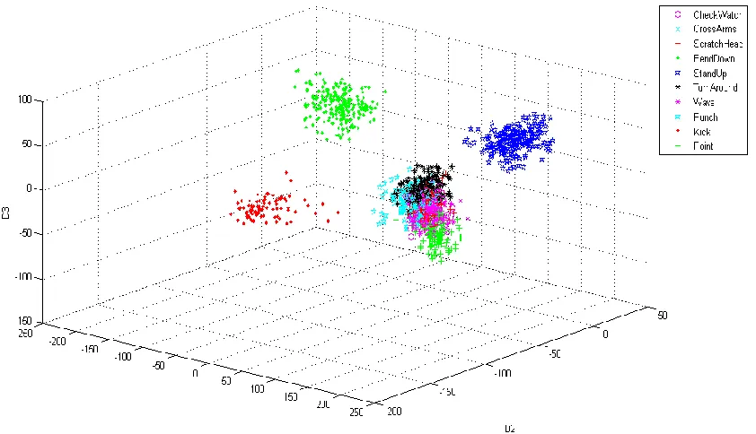
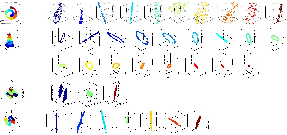
Figure 2-7 shows the 3D embedding of high dimensional radial distance surface actions.

Ten actions were trained using manifold learning reducing 5,000 dimensions down to only three

dimensions for visual illustration. As shown in Figure 2-7, there are clear separations between

activities independently of the view in a 3D space. Point, kick, Bend down, and stand-up were

the most discriminative but the remaining actions, although clustered, do overlap with each other

(28)

19 | P a g e Figure 2-7: The 3D embedding for trained activities from the IXMAS dataset. The actions

are Check Watch, Cross Arms, Scratch Head, Bend Down, Stand Up, Turn Around, Wave,

Punch, Kick, and Point.

CHECK

WATCH

CROSS

ARMS

SCRATCH

HEAD

BEND

DOWN

STAND

UP TURN WAVE PUNCH KICK POINT

CHECK WATCH 0.80 0.20

CROSS ARMS 0.91 0.09

SCRATCH HEAD 0.92 0.08

BEND DOWN 1.00

STAND UP 1.00

TURN AROUND 0.13 0.04 0.04 0.79

WAVE 1.0

PUNCH 0.08 0.92

KICK 1.0

POINT 0.10 0.90

Table 1: Confusion matrix for 1-NN with a 92.48% average accuracy using LPP and radial distance surfaces on the IXMAS dataset.

Table 1 shows the confusion matrix results after testing new data against the trained data

[image:28.612.94.515.73.315.2]

(29)

20 | P a g e accuracy was 92.48% with turn around being the most difficult action to classify. The accuracy

with 3 nearest neighbor and 5 nearest neighbor is 93.23% and 93.98% respectively.

Overall the results look promising with the highest recognition rates using the 5-nearest

neighbor classifier. The biggest challenge is finding a clear separation between similar activities.

For example, scratch head and wave can be confused because both actions require the act of

raising an arm towards the head and, since the viewpoint the action is being captured from is not

fixed, there is potential for confusion. The classification of the turning around action has a high

error rate because the radial distance measure is not effective in capturing useful information of

this action over time. With actions such as punching and kicking, the radial distance surface plot

indicates a significant change while the turning around surface plot is not as descriptive.

2.3.3 3D Joint Descriptor Surfaces

Radial distance features collect descriptive information for 2D images, but do not take advantage

of the information provided by the depth dimension in the 3D depth maps. For example, actions

such as a forward punch (punch towards the camera) are poorly described by the silhouette, but

are described much better with depth data. The 3D joint coordinates, that are available through

the Microsoft Kinect interface software, were selected to capture the depth dimension. The 3D

joint coordinates were calculated using the approach proposed by Shotton et al. [34], where 3D

positions of body joints are predicted from a single depth camera using randomized decision

forest classifiers for body part labeling. Specifically, mean-shift is used to classify each pixel in

an image using spatial mode distribution along with the randomized decision forests to propose

(30)

21 | P a g e The Microsoft Research 3D Dataset (MSRAction3D) (Section 7.2.4) includes the 3D joint

data comprised of 20 coordinates of joint positions in a frame along with their corresponding

depth value and confidence level. The joint positions include the locations of hands, wrists,

elbows, shoulders, the head, the shoulder center, the spine, the hip center, the hips, the knees, the

ankles, and feet. These kinematic coordinates are captured into a feature vector after the joint

coordinates are subtracted from the center torso of the human to define relative data and account

for localization invariance. The difference between the coordinates and the torso coordinates are

then normalized to define features which are scale invariant.

Figure 2-8 shows examples of joint positions on sample frames of a subject performing a

tennis swing action. The 2D coordinates of the joints are normalized individually from the depth

values and the coordinates and the depth data are vectorized into a 1D feature vector of 60

features (20 x-values, 20 y-values, and 20 depth values).

Figure 2-8: Video depth sequences from the MSRAction3D dataset with 3D joint tracking on a subject executing a tennis swing action.

The 3D joint descriptors only represent spatial structures of an instance of time of human

pose. Temporal structuring is necessary to capture the description of an entire action, but it is

known that actions can vary in execution time. To account for time variations we created surface

plots from the feature descriptors which capture the entire action and normalize the surface

(31)

22 | P a g e execution time. Our approach is presented in [48] and is inspired from our earlier work in [13].

Figure 2-9 presents an example of a 3D joint tracking surface representing a tennis swing action.

Figure 2-9: The normalized 3D joint tracking surface for a tennis swing action from the MSRActrion3D dataset.

2.3.4 Radial Distance Surfaces and 3D Joint Surface Descriptor Evaluation

In [48], an evaluation was made using radial distance surfaces, 3D joint surfaces, and a combined

larger representation of both descriptors as one representation. LPP was used as the manifold

learning method with a nearest neighbor classifier on the MSRAction3D dataset consisting of

depth map sequences. There are ten subjects of varying shapes and sizes performing twenty

actions two to three times at various speeds. The dataset actions are listed in Table 2 which is

organized in the same experimental setup as [36]. The 20 actions were divided into three subsets

consisting of 8 actions each. Additionally, we also tested against the entire set of activities

(subset 4). The subsets 1 and 2 were designed to group activities with similar movements while

the third subset was designed to group actions that are more likely to be error prone due to their

similarities. In our experiments, we considered cross validation through random selection and

training and testing with half of the data samples as well as leave one subject out training.

0 20

40 60

0 20

400 0.5 1

# of Features Time

M

a

g

n

itu

d

(32)

23 | P a g e

Subset 1 Subset 2 Subset 3 Subset 4

Hor. Arm Wave Hammer Forward Punch High Throw Hand Clap Bend Tennis Serve Pickup & Throw

High Arm Wave Hand Catch

Draw X Draw Tick Draw Circle Two Hand Wave

Forward Kick Side Boxing High Throw Forward Kick Side Kick Jogging Tennis Swing Tennis Serve Golf Swing Pickup & Throw All Actions

Table 2: The MSRAction3D action subsets used for action classification experiments.

Radial Distance

3D Joint Tracking

Radial Distance & 3D Joint Tracking

Cross Validation

Subset 1 78.31% 84.34% 87.95% Subset 2 74.47% 77.66% 78.72% Subset 3 91.58% 98.95% 98.95% Subset 4 65.09% 73.71% 73.28%

Leave One Subject Out

Subset 1 89.01% 77.65% 92.34% Subset 2 73.73% 74.45% 80.01% Subset 3 85.05% 91.70% 92.98% Subset 4 67.00% 76.14% 76.49%

Table 3: Action classification accuracy on the MSRAction3D dataset. Cross validation and leave one subject out testing were used with radial distance measures, 3D joint tracking, and a combined descriptor.

As presented in Table 3, the combination of radial distance surfaces with 3D joint tracking

meets or exceeds the classification accuracy of either radial distances or 3D joint tracking

independently. In subset 1 where actions were grouped because of their similarities, we achieve

92.34% accuracy using leave one subject out which indicates that the approach is strongly

invariant to individual size, shape, location in a scene, and action execution time which is what

(33)

24 | P a g e subset 3 which was intended to evaluate similar activities. This demonstrates that manifold

learning on descriptor surfaces are strong in classifying similar activities and are therefore highly

discriminative.

Through cross validation the most problematic action to classify for 3D joint tracking was

draw X which frequently got confused with horizontal arm wave. For radial distances forward

punch was frequently confused with horizontal arm wave which is understandable since the

radial distances are similar between these depth related actions. The combined descriptor faces

challenges distinguishing between hammer and tennis serve as well as between draw X and

horizontal arm wave. When our training set became larger using the leave one subject out

approach the most challenging action to classify was draw tick which frequently got confused

with hammer and forward punch.

2.4 Motion Images as Action Descriptors

The next contribution is the formulation of spatio-temporal motion surfaces that can be adapted

for multi-view and 3D action classification applications. To avoid the complexity involved with

body part labeling and tracking, motion images are utilized as temporal templates. The

advantages of motion images include simple representations that provide good performance,

ability to represent the direction of motion in a scene, and ability to identify where motion exists

in a scene. Motion images are extended to represent 3D motion for 3D action classification.

These feature representations can be defined into a spatio-temporal descriptor through surfaces

similar to radial distance surfaces. This section presents motion images, motion history surfaces,

(34)

25 | P a g e

2.4.1 Motion Energy Images and Motion History Images

Motion history images are the primary spatial parametric features used in this dissertation for

action classification systems. Proposed by Davis and Bobick [49], Motion History Images

(MHI’s) are temporal templates that are capable of describing where motion exists in a scene and

how the motion is evolving over time. The MHI features are based on Motion Energy Images

(MEI’s) which offer a binary representation of where motion occurs in a scene. It is an indicator

of motion over time. Given a video frame 𝐼(𝑥, 𝑦, 𝑡), calculate a binary image 𝐷(𝑥, 𝑦, 𝑡) as the difference image between 𝐼(𝑥, 𝑦, 𝑡) and 𝐼(𝑥, 𝑦, 𝑡 ± ∆) where ∆ is a time offset. The binary MEI

𝐸_𝜏(𝑥, 𝑦, 𝑡) is defined as:

𝐸_𝜏(𝑥, 𝑦, 𝑡) = ⋃ 𝐷 𝜏−1

𝑖=0

(𝑥, 𝑦, 𝑡 − 𝑖) (5)

where τ is the temporal extent of the action. This equation captures motion across τ. An example

of MEI’s is shown in the second row of Figure 2-10.

MHI’s capture how motion changes over time in addition to where motion changes over

time. The MHI descriptor 𝐻𝜏(𝑥, 𝑦, 𝑡)⁡is defined as:

𝐻_𝜏(𝑥, 𝑦, 𝑡) = {_{max(0, 𝐻}𝜏⁡⁡𝑖𝑓⁡𝜓(𝑥, 𝑦, 𝑡) = 1

𝜏(𝑥, 𝑦, 𝑡 − 1) − 𝛼)⁡𝑜. 𝑤. (6)

where 𝜏 describes the initial motion response, the decay operator is regulated by 𝛼, and 𝜓(𝑥, 𝑦, 𝑡)

is an update function. There are many variants of update functions [8] including background

subtraction, image differencing, and optical flow. Sample motion history images in Figure 2-10

are shown using a background subtraction update function. The MHI shows more recent motion

appearing brighter than older motion. A main advantage of MHI is that the results represent the

(35)

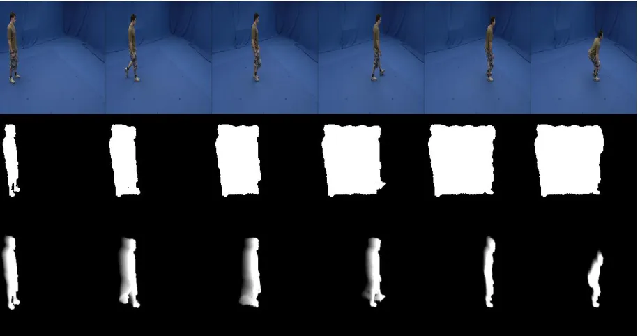
26 | P a g e Figure 2-10: A subject from the i3DPost Multi-View dataset walking across a scene and then sitting. The second row shows the corresponding Motion Energy Images and the third row shows the corresponding Motion History Images with 𝝉 = 𝟕.

2.4.2 Motion History Surfaces

The MHI descriptor is useful in identifying spatial and temporal structuring of actions, however,

the MHI representations in their current form do not easily allow for comparisons between

various actions. Actions vary in terms of the time of execution making it difficult to formulate

an action classification method. Furthermore, human subjects executing such actions can vary in

size and their style in performing actions. It is desired to formulate an action template as one

large representation of an action of a fixed size that can be invariant to scale, position in a scene,

and action execution time.

To do so, spatio-temporal action surfaces are composed from MHI primitives that can

account for these factors. Regions of interest (ROI) of a scene are identified where the motion

[image:35.612.77.536.73.314.2]

(36)

27 | P a g e resized using bicubic interpolation. Figure 2-11 demonstrates an example frame of a subject

walking and the resulting fixed size representation of that frame.

Figure 2-11: An instance of time of an i3DPost multi-view scene of an individual walking in MHI form. The top row shows the original frame. The second row shows the bounding boxes around the region of interest. The bottom row shows a fixed size representation of that same subject.

These fixed size action primitives offer spatial representations but do not identify any

temporal structuring beyond the MHI representation of each action primitive at one instance of

time. To formulate spatio-temporal action templates, we collect entire action sequences and

concatenate the MHI descriptors to form motion history surfaces. In this formulation, the motion

history surfaces become spatio-temporal action templates. These surfaces are normalized using

Equation (7) to encourage minimum scale variations while preserving relative frame information.

Action surfaces can vary due to the execution time of an action by an individual. To account for

time invariance, these surfaces are resized using bicubic interpolation. Azary and Savakis

propose motion history surfaces in [50] for multi-view action classification systems. Radial

(37)

28 | P a g e systems in [48]. Spatio-temporal action surfaces for an individual walking across multiple views

are shown in Figure 2-12.

𝐻_𝜏′ = 𝐻𝜏

𝑚𝑎𝑥_{𝑥,𝑦,𝑡}(𝐻_𝜏) (7)

(38)

29 | P a g e

2.4.3 Motion Depth Surfaces

For 3D video sequences, we use Motion Depth Surfaces (MDS’s) by incorporating the additional

dimension of depth. Assuming 𝐼(𝑥, 𝑦, 𝑡) represents a depth value at pixel (𝑥, 𝑦) for time 𝑡, we

define a motion depth image (MDI) as follows:

𝑀𝐷𝐼_𝜏(𝑥, 𝑦, 𝑡) = {_{max(0, 𝑀𝐷𝐼}𝐼(𝑥, 𝑦)⁡⁡𝑖𝑓⁡𝐷(𝑥, 𝑦, 𝑡) = 1

𝜏(𝑥, 𝑦, 𝑡 − 1) − 𝛼) (8)

This formulation permits us to capture motion activity in the depth direction as well as

within a frame. We concatenate each MDI to create a motion depth surface (MDS) that

represents spatio-temporal motion with built-in depth motion. As was done with MHS, these

surfaces were scaled to a fixed size to account for variations in the timing of actions and to

ensure that the number of dimensions of each action descriptor remains consistent and its size is

manageable.

Examples of subjects executing a horizontal arm wave and a forward punch from the

MSRAction3D dataset shows how the direction of depth is incorporated into the MDS descriptor

as shown in Figure 2-13. Similarly, Figure 2-14 shows a comparison of an MHS and an MDS

description of the ASL gesture for Green from the MSRGesture3D dataset.

(39)

30 | P a g e

Forward Punch

Figure 2-13: A comparison of MHI (top rows) with MDI (bottom rows) for subjects performing a horizontal arm wave action and a forward punch from the MSRAction3D dataset.

a)

b)

(40)

31 | P a g e

3 Dimensionality Reduction Methodologies

The high dimensional data that represent an action or a face can become overwhelming when

dealing with a large number of data samples. A common challenge for real-world classification

and recognition systems is the computational performance associated with processing

high-dimensional data. Subspace learning high-dimensionality reduction addresses the issue of high

dimensional data by finding an efficient low-dimensional representation. The following sections

focus on dimensionality reduction methods including principal component analysis (PCA),

metric multidimensional scaling (MDS), local linear embedding (LLE), and linear extensions of

graph embedding (LGE).

3.1 Principal Component Analysis

Principle Component Analysis (PCA) is a widely used methodology for reducing the dimensions

of complex and/or noisy data sets to extract relevant information that can be beneficial in

describing the data. It is a linear technique that projects data along the directions of maximal

variance. PCA has been employed for action classification systems in several works including

[51] and [52]. In this section, PCA is overviewed, including its benefits and limitations, as

outlined in [53] and [54]. For data sets with large number of samples n the information can be

computationally expensive to process. PCA aims to reduce noise and redundancy while

preserving the global structure of the high dimensional data [55] by preserving the maximal

variance. Given 𝑛-samples of data 𝑿, eachof 𝑚-dimensions, PCA provides a way to calculate

a lower dimensional representation 𝒀 of the higher dimensional data through a transformation 𝒀′ = 𝑷′𝑿. To solve for this transformation, PCA calculates a square covariance matrix. PCA

(41)

32 | P a g e covariance matrix to identify principal components of maximal variance. An alternative

approach to finding the eigenvectors involves Singular Value Decomposition (SVD).

PCA is a linear method for extracting linear features based on maximal variance. When the

data set is a representation of non-linear features, the principal components may not be effective

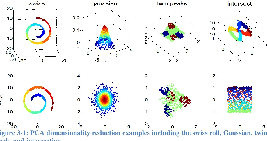
in simplifying the data set successfully. For an illustrative example, four 3D shapes are

presented in Figure 3-1. The first row shows the original 3D representations: swiss roll,

Gaussian, twin peaks, and intersect. The colors identify classes associated with each sample.

The 2D representations after applying principal component analysis are shown in the second

row. PCA performs well in representing the swiss roll and Gaussian surfaces, but the other more

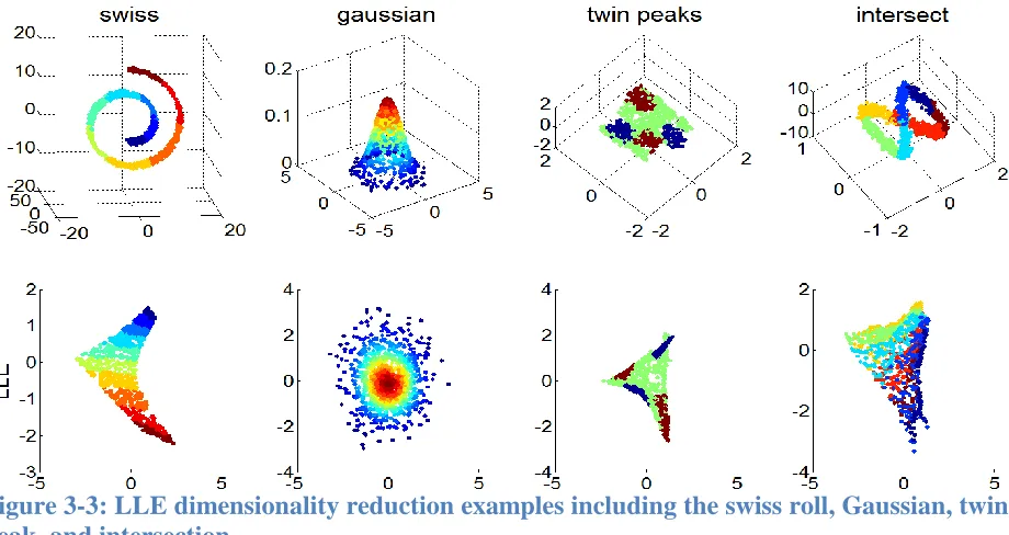
[image:41.612.80.539.375.618.2]

complex shapes do not show a consistent pattern of within class clustering.

(42)

33 | P a g e Given 𝑛 as the number of data samples and 𝑝 as the number of classes, the covariance matrix

computation of PCA has a time complexity of 𝑂(𝑝2𝑛). The eigenvalue decomposition has a time complexity of 𝑂(𝑝3_{). Therefore, PCA has a time complexity of 𝑂(𝑝}2_{𝑛 + 𝑝}3_{) [56].}

3.2 Metric Multidimensional Scaling

Metric Multidimensional Scaling (MDS) is a linear technique for dimensionality reduction based

on proximity data analysis. MDS attempts to define a distance measure between data in the high

dimensional space that would be preserved in a lower dimensional space and is a good identifier

of clustering patterns. MDS has been used for a wide variety of applications including stock

market analysis [57], wireless sensor network localizations [58], and protein binding predictions

[59].

Given a data set 𝑿 = {𝑿_𝟏, 𝑿_𝟐, … , 𝑿_𝒏}for which each element in the data set resides in a high

dimensional space 𝐵 such that 𝑿𝑖 ∈ ℝ𝐵, MDS will solve for a lower dimensional representation

set 𝒀 = {𝒀1, 𝒀2, … , 𝒀𝑛} in space 𝑏 such that 𝒀𝑖 ∈ ℝ𝑏 and 𝑏 ≪ 𝐵. This mapping is approximated

by the distances between samples following ‖𝑿_𝑖− 𝑿_𝑗‖ [60]. A square dissimilarity matrix is

created which measures the distance between each pair of elements in the high dimensional

space as demonstrated in Equation (9) with 𝐷_𝑖𝑖 = 0 and 𝐷_𝑖𝑗 > 0.

𝑫 = [

𝐷11 ⋯ 𝐷1𝑗

⋮ ⋱ ⋮

𝐷_𝑖1 ⋯ 𝐷_𝑖𝑗] (9)

The Minkowski distance metric [61] shown in Equation (10) is a general distance measure

between elements where n is the number of data samples. This equation is transformed to the

(43)

34 | P a g e Such distance measures can be used as proximity measures in the high dimensional space

depending on the application.

𝐷𝑖𝑗 = [∑|𝑿𝑖𝑘 − 𝑿𝑗𝑘|𝑟 𝑛 𝑘=1 ] 1 𝑟 (10)

Given the dissimilarity matrix 𝑫, the MDS problem becomes a minimization problem for which we desire a transformation that will minimize the error of the distances in a lower

dimensional space. To do this we use the following stress function as a least squares criterion.

The stress function 𝑆𝐷(𝑿1, 𝑿2, … , 𝑿𝑛) in Equation (11) measures the deviation between the distance 𝐷_𝑖𝑗 and the target distance ‖𝑿_𝑖 − 𝑿_𝑗‖.

𝑆_𝐷(𝑿1, 𝑿2, … , 𝑿𝑛) = √∑ ∑(𝐷𝑖𝑗 − ‖𝑿𝑖 − 𝑿𝑗‖) 2 𝑛 𝑗=1 𝑛 𝑖=1 (11)

Equation (12) shows the minimization function that minimizes the stress over all points

while finding the transformation that will reduce the number of dimension from 𝐵 to 𝑏 such that

𝑏 ≪ 𝐵[63].

min

𝑌 ∑ ∑ (‖𝑿𝑖 − 𝑿𝑗‖ 2

− ‖𝒀_𝑖 − 𝒀_𝑗‖2)2 𝑛

𝑗=1 𝑛

𝑖=1

min

𝑌 ∑ ∑(𝐷𝑖𝑗 𝑋_{− 𝐷}

𝑖𝑗𝑌) 2 𝑛 𝑗=1 𝑛 𝑖=1 (12)

The method of minimization with metric multidimensional scaling is an eigenvalue problem.

The distance matrix 𝑫𝑋_{is converted to a matrix of inner products}_{𝑿′𝑿 which reduces Equation}

(12) to Equation (13).

min

𝑌 ∑ ∑(𝑿𝑖 ′_𝑿

𝑗 − 𝒀𝑖′𝒀𝑗)2 𝑛

𝑗=1 𝑛

𝑖=1

(44)

35 | P a g e The eigenvectors 𝑽 of 𝑿′𝑿 are used to solve for the top 𝑚 eigenvalues, 𝝀. The coordinates

are transformed from high dimensional space 𝐵 with 𝑿_𝑖 ∈ ℝ𝐵_{to lower dimensional space 𝑏 with}

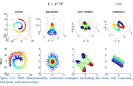
𝒀𝑖 ∈ ℝ𝑏 following Equation (14). Figure 3-2 shows the 2D representations of 3D shapes that were reduced through MDS using a Euclidean distance metric (𝑟 = 2).

𝒀 = 𝝀1/2_𝑽′ ₍₁₄₎

Figure 3-2: MDS dimensionality reduction examples including the swiss roll, Gaussian, twin peak, and intersection.

The lower dimensional representation of the training data only represents the original high

dimensional training data and it is unclear how to map new testing data samples. For this reason,

MDS is ideal for proximity and cluster analysis, but is not ideal for systems requiring the

classification of new data samples. The computational complexity of MDS is 𝑂(𝑛3_{) [64].}

3.3 Locally Linear Embedding

Locally Linear Embedding (LLE) is an unsupervised eigenvector method for dimensionality

reduction that preserves the embedding of high dimensional data through maximal

[image:44.612.77.542.179.479.2]

(45)

36 | P a g e structure of the manifold. LLE has been used for a wide variety of applications including the

mapping of DNA gene expressions [65] and super resolution [66].

Given a data set 𝑿 = {𝑿₁, 𝑿₂, … , 𝑿_𝑛} for which each element in the data set resides in a high

dimensional space 𝐷 such that 𝑿_𝑖 ∈ ℝ𝐷, LLE maps 𝑿 to a lower dimensional representation new data set 𝒀 = {𝒀₁, 𝒀₂, … , 𝒀_𝑛} for which each element in 𝒀 resides in a lower dimensional

space 𝑑 such that 𝒀𝑖 ∈ ℝ𝑑 and 𝑑 ≪ 𝐷. LLE uses multiple stages for this mapping. First, it computes the nearest neighbors of each data point 𝑿_𝑖. Then, it constructs a weight matrix 𝑾_𝑖𝑗 between all data points 𝑿𝑖 that represent the local linear geometry. Weights are assigned a value

of zero for the pairs that are not considered nearest neighbors. Nearest neighbor weights are

computed in a manner that can best reconstruct each data point from its neighbors in the lower

dimensional space. This is accomplished by establishing measurement of reconstruction errors

based on the cost function of Equation (15). This cost function identifies how well each 𝑿_𝑖 can be linearly constructed from its nearest neighbors 𝑿_𝑁(1)… 𝑿_𝑁(𝑘) [67].

𝜀(𝑊) = ∑ |𝑿𝑖 − ∑ 𝑾𝑗(𝑖)𝑿𝑁(𝑗) 𝑘

𝑗=1

| 2 𝑛

𝑖=1

(15)

This cost function is designed to ensure invariance to rotation and scale [68]. The constraint

∑𝑘𝑗=1𝑾𝑗(𝑖)= 1 ensures the sum of the weights between 𝑿𝑖 and all selected neighbors will sum to

1 and be invariant to translation. The cost function can then be treated as a constrained least

squares problem to solve for the optimal weights. These weights represent the local linear

geometry of the patches since they were determined by assigning weights of the nearest

(46)

37 | P a g e Φ(𝑌) = ∑ |𝒀𝑖 − ∑ 𝑊𝑗(𝑖)𝒀𝑁(𝑗)

𝑘

𝑗=1

| 2 𝑛

𝑖=1

(16)

Constraining ∑ 𝒀𝑖 𝑖 = 0 and 1⁄ ∑ 𝒀_𝑁 𝑖 𝑖′𝒀𝑖 = 𝐼 results in the following cost function.

Φ(𝑌) = ∑|(𝑰 − 𝑾)𝒀_𝑖|2 _{= 𝑡𝑟(𝒀′𝑴𝒀)} 𝑛

𝑖=1

(17)

where 𝑴 ∈ 𝑅𝑁×𝑁 and 𝑴 = (𝑰 − 𝑾)′(𝑰 − 𝑾). The final step of LLE is to compute the bottom non-zero eigenvalues of matrix 𝑴.

Similar to MDS, the lower dimensional representation of the training data only represents

the original high dimensional training data and it is unclear how to map new testing data

samples. For this reason, LLE is ideal for preserving the embedding of high dimensional data

through maximal discrimination and analyzing clustering patterns, but not ideal as a method for

learning and classifying new test data. Figure 3-3 illustrates the 2D mappings of 3D shapes.

Notice how the shapes are clustered in patches. The time complexity of LLE is a sum of

searching the nearest neighbors 𝑂(𝐷𝑛3), computing the reconstruction weights 𝑂(𝐷𝑛𝑘3), and

Grassmann Learning for Recognition and Classification

RIT Scholar Works

Grassmann Learning for Recognition and

Classification

Grassmann Learning for Recognition and

Classification

Abstract

Acknowledgements

Table of Contents

1

Introduction

2

Representations for Action Classification and Face Recognition

3

Dimensionality Reduction Methodologies