Comparative analysis of two variants of the Knox test: Inferences from space-time pattern analysis

This is a repository copy of Comparative analysis of two variants of the Knox test:

Inferences from space-time pattern analysis.

White Rose Research Online URL for this paper:

http://eprints.whiterose.ac.uk/124149/

Version: Accepted Version

Proceedings Paper:

Adepeju, MO orcid.org/0000-0002-9006-4934 and Evans, A

orcid.org/0000-0002-3524-1571 (2017) Comparative analysis of two variants of the Knox

test: Inferences from space-time pattern analysis. In: Gervasi, O, Murgante, B, Misra, S,

Borruso, G, Torre, CM, Rocha, AMAC, Taniar, D, Apduhan, BO, Stankova, E and

Cuzzocrea, A, (eds.) Lecture Notes in Computer Science. 17th International Conference

on Computer Science and Its Applications (ICCSA 2017), 03-06 Jul 2017, Trieste, Italy.

Springer Nature , pp. 770-778. ISBN 978-3-319-62407-5

https://doi.org/10.1007/978-3-319-62407-5_59

(c) 2017, Springer International Publishing AG. This is an author produced version of a

paper published in Lecture Notes in Computer Science. Uploaded in accordance with the

publisher's self-archiving policy. The final publication is available at Springer via

https://doi.org/10.1007/978-3-319-62407-5_59

[email protected] https://eprints.whiterose.ac.uk/

Reuse

Items deposited in White Rose Research Online are protected by copyright, with all rights reserved unless indicated otherwise. They may be downloaded and/or printed for private study, or other acts as permitted by national copyright laws. The publisher or other rights holders may allow further reproduction and re-use of the full text version. This is indicated by the licence information on the White Rose Research Online record for the item.

Takedown

If you consider content in White Rose Research Online to be in breach of UK law, please notify us by

ICCSA, p. 1, 2017.

© Springer-Verlag Berlin Heidelberg 2017

Comparative analysis of two variants of the Knox test:

Inferences from space-time crime pattern analysis

1_{Monsuru Adepeju (0000-0002-9006-4934) and} 2_{Andy Evans}

(0000-0002-3524-1571)

1,2 _{School of Geography, University of Leeds, LS2 9JB, United Kingdom}

1_{[email protected]}

2_{[email protected]}

Abstract. This paper compares two variants of the Knox test in relation to space-time crime pattern analysis. A case study of stolen-crime data sets of San Francisco city is presented. The comparative analysis shows that while one variant is designed to detect the sizes of the spatio-tem-poral neighbourhoods at which clustering (hotspots) is prominent within a data set, the other variant is able to reveal the spatial and temporal win-dows/bands at which crime events are frequently repeated to form clusters (hotspots) across an area.

Keywords: Knox test, space-time, crime, repeat pattern, critical distances.

1

Introduction

each dimension (Fig. 1b), relative to a reference point . As a revised version, the binned neighbourhood is intended to filter out anomalous highs which are less likely to result from interactions due to .

The Knox test has been widely used for the purpose of understanding the space-time pattern of crime data sets, particularly the repeat and near-repeat (RNR) pattern (Farrel and Pease, 1993). The RNR is the concept that if a loca-tion is the target of a particular crime type, such as burglary, the houses within a relatively short distance of it have an increased risk of being burgled over a period of a limited number of weeks (Bowers and Johnson, 2004). While both variants of the Knox test have been used to describe the RNR patterns, there is yet to be any empirical studies that compare such results, and further, to highlight their relationship with regards to the space-time patterns displayed by the data set. Therefore, the purpose of this study is to address this research gap. For a comprehensive comparison, each variant of the Knox test will be used to examine the space-time pattern in relation to two different crime types, using a list of neighbourhood values.

2

The Knox test and the space-time neighbourhood definition

The Knox test looks at the relationships between all pairs of events in a spatio-temporal dataset, generating a test statistic ( ,) that is larger when, for ample, short space-time distances appear more frequently than would be ex-pected by chance (indicating RNR behaviour). The test statistic is generated from a table where spatial and temporal distances are binned and pairings al-located to the cells. Rather than testing all possible combinations, it is usual to pass a moving window repeatedly over the data point-by-point, varying the critical spatial and temporal widths, measured from the moving reference point, r; the variation size corresponding to the bins in the table. This allows only events within a reasonable space/time distance of to be taken, improving calculation speeds. Structuring the window to remove sections allows for more complicated distance filters, as is the case in the

. A closeness matrix describes the closeness of all pairs of events, either in space or in time. Thus, one matrix is created for closeness in space and the other for closeness in time. For the first matrix, an will

have an entry 1 for the cell if event occurred within some spatial dis-tance of the event and 0 otherwise. The spatial closeness is calculated by the 2D Euclidean distance measurement. Similarly for the second matrix, a will have an entry 1 for the cell if the event occurred within some

temporal distance of the event and 0 otherwise. The temporal closeness is calculated by the difference between the times of occurrences of any pair of events. Both matrices would have a dimension , where is the total number of point events. For both matrices, if , then the entry is 0. The test statistic is then formulated by the cross-product:

(1)

if the distance between cases i and j otherwise

if the distance between cases i and j otherwise

number of simulations. Here we utilise this MC process. The MC process is ex-tremely computationally intensive, thus, a parallel computing approach, in which multiple analyses are run simultaneously, was used.

2.1 Types of space-time neighbourhoods

The parameters and described above can be referred to as the spatial and temporal neighbourhoods, respectively, within which events that fall inside are considered close . This is the original version of the Knox test, as proposed by Knox (1964). In this study, this was referred to as an enclosed

neighbourhood variant. In other words, an enclosed _{neighbourhood involves}

counting events within a region defined by critical spatial ( ) and a critical tem-poral ( ) distances, measured from a reference point (Fig. 1a). A revised neighbourhood definition was later proposed (Knox 1963), in which event counts are conducted within a region, which are created by the subtraction of the two distances measured along each dimension. In this version of the Knox test, the resulting neighbourhood is referred to as the binned _{neighbourhood}

(Fig. 1b).

Fig. 1. Two types of neighbourhood definitions for the Knox test. (a) Enclosed neighbourhood, (b) Binned neighbourhood: each dimension requires two of and to form the region (i.e. { and } and { and }, respectively). The cases count in (a) is 8, while the cases count in (b) is 6 (Diagram from: Adepeju et al., 2017).

Thus, for the binned _{neighbourhood, two critical distances { and } and {}

The above two neighbourhood definitions, that is, the enclosed

neighbour-hood and the binned _{neighbourhood, underlie the two variants of the Knox}

test and will be used in this study.

In the crime domain, a contingency table is usually created in which the Knox test is repeatedly run using different values of and , and the contingency table is populated accordingly. The values of and are usually set arbitrarily. Although most studies often justify the value they use from a theoretical and/or practical point of view. In this study, the primary focus is to compare the two variants as regards to long-term local neighbourhood crime preven-tion. Therefore, the values of and will be made to vary at 30 day interval and 200m in the temporal and spatial dimensions, respectively. In the case of the binned variant, the inner bin is set such that the neighbourhood created with the outer bin is of 30 days and 200m in the temporal and spatial dimen-sions, respectively.

3

Case study of San Francisco crime data sets

3.1 Data sets

The data for this study are the - crimes in San Fran-cisco, CA, U.S.A, for the year 2015. During this year, the city had some of the

-of-motor-vehicles at approximately 20% and 150%, respectively, higher than the national average. The burglary and -vehicles s 4,267 and 4,970 records, respectively. From January to September, the monthly count of burglary crime looks very similar, with the exception of May, which is ~15% higher than the monthly average

(Fig. 2a) O - for

Fig. 2. Monthly crime count

3.2 P repeat patterns

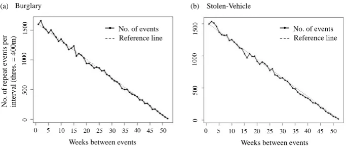
In crime pattern analysis, a common approach for visualising the repeat and near repeat (RNR) pattern in crime data sets is to draw the repeat pattern pro-file (Johnson et al., 1997). The propro-file is drawn by counting the number of crimes occurring within a space and time lapse. The profile usually provides a picture of how events are repeated within a time window in a defined neigh-bourhood size, across the entire area. This same idea underlies the Knox test, except that the Knox test incorporates the statistical significance evaluation. Examples of repeat pattern profiles are shown in Fig. 3.

Fig. 3. Repeat pattern profile. (a) and

len-

Jan Apr Jul Oct Dec Jan Apr Jul Oct Dec

Month Month Burglary Stolen-Vehicle Freq u en c y Avg. Avg. (a) (b)

Weeks between events

Burglary No . o f re p ea t ev en ts p er in ter v al (t h re s. = 4 0 0 m

) No. of events_{Reference line}

0

500

1000

1500

0 5 10 15 20 25 30 35 40 45 50

Weeks between events

0

500

1000

1500

0 5 10 15 20 25 30 35 40 45 50

Reference line No. of events

Fig. 3 shows the repeat pattern of the data set, measured within a neighbour-hood of 400m in radius of an initial event. A relatively high level of repeats is indicated by the undulations in the profiles. A reference line is created in order to make the undulations (repeats) more visible by joining the first and last event. In Fig. 3a, it can be observed that the repeat pattern is more prominent in the first five months of burglary crime, while the repeat extends up to the sixth - T can be easily be inferred that the repeat of crimes is prominent in the first five months for both crime types. However, the statistical quantification is missing in this type of analysis. This is where the Knox test plays an important role.

4

Results and Discussion

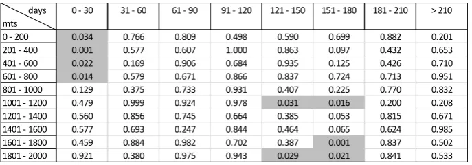
Table 1 and Table 2 shows the results of the two variants of the Knox test for the burglary and n- T results for the en-closed neighbourhood variant and binned neighbourhood variant are pre-sented in table labelled (a) and (b). Highlighted values indicate where the pseudo p-value is smaller than 0.05, meaning that the likelihood of it occurring by chance is less than one in 20.

Table 1a: The enclosed neighbourhood variant Knox test: Burglary crime

Table 1b: The enclosed _{neighbourhood variant Knox test: Stolen-vehicle}

days mts

0 - 30 0 - 60 0 - 90 0 - 120 0 - 150 0 - 180 0 - 210 0 - 240

In Tables 1a and 1b, representing the results of the enclosed neighbourhood variant of Knox test, all the cells with statistically significant values are ar-ranged close to one another. In both cases, as the statistically significant cells extend in temporal sizes from 30 to 120 days, the corresponding spatial sizes decreases. This pattern indicates that significant levels of events are much closer in space at much smaller temporal sizes than at larger temporal sizes, larger distances and times being associated with events which blend with background noise. The relative closeness of events, simultaneously in both space and time, is generally referred to as space-time clustering (Diggle and Chetwynd, 1995). Considering the construct of the enclosed neighbourhood, as shown in Fig. 1a, it is argued that this variant of the Knox test is suited to

the detection of

time. In other words, we can say that space-time clustering of events is being detected (Diggle and Chetwynd, 1995). Specifically, it detects the critical spa-tial and temporal distances at which events concentrations are statistically significant, and thus, form space-time clusters (hotspots). These critical spatial and temporal distances can then be described as the spatial and temporal scales of the most prominent clusters within the data set.

Table 2a: The Binned _{neighbourhood variant Knox test: Burglary crime}

days mts

0 - 30 0 - 60 0 - 90 0 - 120 0 - 150 0 - 180 0-210 0-240

0 - 200 0.031 0.035 0.202 0.448 0.466 0.515 0.663 0.85 0 - 400 0.002 0.001 0.003 0.026 0.615 0.762 0.65 0.744 0 - 600 0.001 0.001 0.002 0.039 0.397 0.638 0.488 0.503 0 - 800 0.001 0.001 0.003 0.059 0.394 0.621 0.55 0.631 0 - 1000 0.001 0.021 0.005 0.117 0.465 0.625 0.556 0.593 0 - 1200 0.009 0.042 0.128 0.436 0.834 0.801 0.678 0.72 0 - 1400 0.036 0.061 0.249 0.574 0.829 0.798 0.664 0.727 0 - 1600 0.054 0.054 0.371 0.558 0.845 0.803 0.635 0.684 0 - 1800 0.059 0.071 0.438 0.677 0.859 0.832 0.643 0.712 0 - 2000 0.097 0.136 0.543 0.771 0.911 0.827 0.665 0.736

days mts

0 - 30 31 - 60 61 - 90 91 - 120 121 - 150 151 - 180 181 - 210 > 210

Table 2b: The Binned K “ -vehicle crime

In Tables 2a and 2b, representing the results of the binned neighbourhood variant of the Knox test, all the cells with statistically significant values are dis-jointed and distributed within four temporal bands, namely: {0-30 days}, {31-60 days}, {121-150}, and {151-180}. The critical spatial distances of the cells against their corresponding critical temporal distances can be described as the spatial and temporal windows at which there are more interactions or repeats in the data set. Two events interact when they are at a distance from one an-other in space and time different from that which would be expected on ag-gregate on the basis of chance. In both crime types, events are clustered within the first 2 months and also within 5 to 6 months of one another, which may be translated as the short-term and long-term repeat patterns. The ability to this variant of the Knox test to clearly isolate repeat patterns in terms of their temporality constitutes its major improvement over the

profile of Fig. 3.

Comparing the general distribution of the significant cells in all the tables, it can be observed that the patterns at smaller spatial and temporal bands/neighbourhoods (i.e. between 0m and 800m) are much stronger, and thus persist across the two variants. On the other hand, the significant cells in the distant bands for the binned variant were not reflected in the enclosed variant, and are thus tagged as weak patterns.

Crime clusters (hotspots) are formed as a result of many crimes interacting within a common neighbourhood. In practice, while the results of the binned neighbourhood variant of the Knox test can be used to identify the spatial and the temporal lags at which the next set of crimes are likely to occur, the results

days mts

0 - 30 31 - 60 61 - 90 91 - 120 121 - 150 151 - 180 181 - 210 > 210

of the enclosed neighbourhood variant of the Knox test can be used to inves-tigate the sizes of the spatial and temporal windows (neighbourhoods) to tar-get during crime intervention over a coherent period after the event. This has advantages in terms of both public fear of crime and utilisation of household-ers fresh commitment to target hardening. While the Knox test is relatively simple and efficient to calculate, a more locally detailed answer as to the struc-ture of short-term spatio-temporal clustering may be obtainable by employing a local clustering test, such as space-time scan statistics (STSS) (Kulldorff et al., 2005). An STSS is able to detect and isolate the specific space-time regions that contribute to the overall clustering derived by a global test such as the Knox test.

5

Conclusions

This study presents a comparative analysis of two variants of the Knox test, distinguished by the manner in which the space-time neighbourhoods (i.e. critical distances) are defined. These two neighbourhood definitions were re-ferred to here as the enclosed _and binned _{neighbourhoods. The goal was to}

compare the results generated by these two variants in relation to the same data set, as well as to describe their relationships from both theoretical and practical perspectives. The data set used for the analysis was the burglary and

-vehicles dataset for the city of San Francisco.

The results reveal that the enclosed _{variant helped to detect the sizes of the}

spatio-temporal neighbourhoods at which clustering (hotspots) was promi-nent within the dataset. The binned _{variant, on the other hand, revealed the}

spatial and temporal windows at which crime events were repeated more broadly to form clusters (hotspots) across an area.

References

1. Adepeju, M., 2017. Modelling of Sparse Spatio-Temporal Point Process (STPP) an appli-cation in Predictive Policing. A PhD thesis submitted to the University College London (2017).

2. Agresti, A. and Finlay, B.: Statistical Methods for the Social Sciences, 3rd edn. New Jersey: Prentice Hall (1997)

3. Bowers, K.J. and Johnson, S.D.: Who commits near repeats? A test of the boost explana-tion. Western Criminology Review, 5(3), 12-24 (2004).

4. Diggle, P.J., Chetwynd, A.G., Häggkvist, R. and Morris, S.E.: Second-order analysis of space-time clustering. Statistical methods in medical research, 4(2), 124-136 (1995).

5. Farrell, G. and Pease, K.: Once bitten, twice bitten: Repeat victimisation and its implica-tions for crime prevention. (1993)

6. Johnson, S.D., Bernasco, W., Bowers, K.J., Elffers, H., Ratcliffe, J., Rengert, G., Townsley, M.: Space-time patterns of risk: a cross national assessment of residential burglary victim-ization. J Quant Criminol,23, 201 219 (2007)

7. Kleinman, K.P., Abrams, A.M., Kulldorff, M. and Platt, R.: A model-adjusted space time scan statistic with an application to syndromic surveillance. Epidemiology and Infection, 133(03), 409-419. (2005).

8. Knox, G.: Detection of Low Intensity Epidemicity Application to Cleft Lip and Palate. Brit-ish journal of preventive & social medicine, 17(3), 121-127 (1963).

9. Knox, G.: Epidemiology of Childhood Leukaemia in Northumberland and Durham. Brit. J. of Prev. and Social Med, 18, 17-24 (1964).

10. Mantel, N.: The detection of disease clustering and a generalized regression approach. Cancer Res., 27, 209 220 (1967).

11. Ohno, Y., Aoki, K. and Aoki, N.: A test of significance for geographic clusters of disease. In-ternational Journal of Epidemiology, 8(3), 273-281 (1979).