Electron localisation in static and time-dependent one-dimensional model systems

one-dimensional model systems.

White Rose Research Online URL for this paper: http://eprints.whiterose.ac.uk/127321/

Version: Accepted Version

Article:

Durrant, T. R., Hodgson, M. J.P., Ramsden, J. D. et al. (1 more author) (2018) Electron localisation in static and time-dependent one-dimensional model systems. Journal of physics : Condensed matter. 065901. ISSN 1361-648X

https://doi.org/10.1088/1361-648X/aaa4cd

[email protected] https://eprints.whiterose.ac.uk/

Reuse

Items deposited in White Rose Research Online are protected by copyright, with all rights reserved unless indicated otherwise. They may be downloaded and/or printed for private study, or other acts as permitted by national copyright laws. The publisher or other rights holders may allow further reproduction and re-use of the full text version. This is indicated by the licence information on the White Rose Research Online record for the item.

Takedown

If you consider content in White Rose Research Online to be in breach of UK law, please notify us by

one-dimensional model systems

T. R. Durrant1‡, M. J. P. Hodgson1§, J. D. Ramsden1, R. W. Godby1

1

Department of Physics, University of York, and European Theoretical Spectroscopy Facility, Heslington, York YO10 5DD, United Kingdom

Abstract. The most direct signature of electron localisation is the tendency of an electron in a many-body system to exclude other same-spin electrons from its vicinity. By applying this concept directly to the exact many-body wavefunction, we find that localisation can vary considerably between different ground-state systems, and can also be strongly disrupted, as a function of time, when a system is driven by an applied electric field. We use this measure to assess the well-known electron localisation function (ELF), both in its approximate single-particle form (often applied within density-functional theory) and its full many-particle form. The full ELF always gives an excellent description of localisation, but the approximate ELF fails in time-dependent situations, even when the exact Kohn-Sham orbitals are employed.

Submitted to: J. Phys.: Condens. Matter

‡ Present Address: Department of Physics and Astronomy and London Centre for Nanotechnology, University College London, Gower Street, London, WC1E 6BT, United Kingdom

1. Introduction

Density functional theory (DFT) [1] replaces the many-body (MB) wavefunction with the electron density as its fundamental variable, making electronic structure problems computationally tractable. However, this transformation provides new challenges, as in the non-interacting world of Kohn-Sham (KS) electrons, the many-body behaviour of electrons is concealed within the exchange-correlation (xc) potential [2].

Electron localisation, describing the tendency of an electron to exclude other same-spin electrons from its vicinity (i.e. position entanglement of like-same-spin electrons), is one such property [3, 4]. Although a commonly used concept, it is not always well defined. We choose to start from the idea that localised electrons tend to avoid one another, whereas delocalised electrons will share the same region of space. Localisation is partly driven by Pauli exclusion, which acts to localise like-spin electrons in separate regions. The Coulomb interaction further enhances the tendency to localise [5]. The electrons’ attempts to avoid each other increase the kinetic energy, which, however, is minimized by spreading electrons over as large a volume as possible. It is the balance between these factors that makes electron localisation challenging to quantify.

An understanding of electron localisation is useful chemically, placing the ubiquitous concepts of chemical bonds and localised electron pairs on a formal footing [6]. Although measures of localisation provide an understanding of bonds and electron pairs made up of electrons of opposite spin, these details are revealed by looking at the localisation oflike-spinelectrons, which provides the regions in which localised opposite-spin electron pairs can be found. Localisation also describes a fundamental aspect of electron correlation that approximate DFT functionals should take into account [7,8, 9,10, 11, 11].

We stress that localisation is a true many-body property of electrons, dependent on the positions of all electrons, and not accessible through the spatial character of any one KS orbital. Although many early efforts focused on the extent of molecular or KS orbitals, it was soon realized that these orbitals are not unique and that quite different choices could be selected [4].

2. Measures of localisation

To calculate our measure, we note that in localised systems each electron will avoid the others by tending to stay in its own region of space. We first partition the system into distinct regions, each containing charge corresponding to one electron, and examine the actual distribution of theN electrons among these regions. To simplify our definition, we consider a wavefunction with only one type of spin. The probability that each of theN

electrons is in adifferent region is calculated using a mask functionM. M(r1, . . . , rN) is defined as 1 wherer1, . . . , rN all lie in distinct regions, and 0 otherwise, and interrogates the probability of such a situation via the N-electron wavefunction Ψ. The probability is then given by

p=

Z

M(r1, . . . ,rN)|Ψ(r1, . . . ,rN)|2d3r1. . . d3rN . (1)

The inclusion of spin replaces the wavefunction with the appropriateN-body same-spin density matrix.

Equation 1 fully defines our measure once a set of one-electron regions is provided via M. In the present paper we study dimensional finite systems, where the one-electron regions inM are straightforwardly identified from the cumulative integral of the electron density: starting from one edge, the system is simply divided into N regions, each containing the charge of one electron. More generally, the set of regions which most faithfully represents how the electrons are localised in the system would be that which maximises Eq. 1k.

To form our regional electron localisation measure (RELM), we scale p with reference to the probability p0 =N!/NN _{of finding exactly one electron in each region}

for an ideal delocalised and uncorrelated state:

RELM = p−p0

1−p0. (2)

This makes our measure 0 when a system is ideally delocalised, and 1 when fully localised. As the probability of simultaneously finding only one electron in each region increases, so does our measure of localisation. As with the ELF, our measure is calculated for each spin index independently.

Of course, in most cases the MB wavefunction, on which the RELM relies, is too expensive to calculate. The traditional method of approximating the localisation in a system is the ELF of Becke and Edgecombe [3]. The following reference provides a comprehensive review of the ELF [4]. Originally developed for Hartree-Fock (HF) calculations, the method can also be applied to Kohn-Sham orbitals. The ELF is based on the quantity Dσ, defined by the Taylor series

ρσσ

Cond(r, s) =

Dσ(r)s2

d +O(s

3_{), (3)}

whereρσσ

Cond is a conditional probability, the probability given that an electron has been

found at positionr that a second electron will be found at distancesfrom this position.

dis the spatial dimensionality of the system andσ is a spin index. Dσ characterises the probability of finding a second (same-spin) electron very close to the reference electron and is a measure of localisation in its own right.

Later work by Dobson [5] provides an equivalent definition ofDσ(r) to that given in Eq.3, allowing this quantity to be calculated directly from the same-spin pair density, using the equation

Dσ(r) =

h

∇2

r′n

σ 2(r,r′)

i

r′=r

2nσ(r) , (4)

where nσ

2(r,r′) is the pair density. Using this expression, it is possible to calculate the

ELF directly from the wavefunction; we term this the “exact ELF”.

As Dσ has a strong dependence on the local density, it is not easily interpreted directly. To produce the ELF, Becke and Edgecombe scaled Dσ as

ELF (r) = 1 1 + Dσ(r)

Dσ,H(r)

2. (5)

This expression compares the local value of Dσ with that of the Hartree-Fock homogeneous electron gas of the same local density,Dσ,H(a convenient reference system against which to compare the actual value ofDσ). Hence, ELF ranges from zero to one, where 1 represents total localisation and 0.5 represents the degree of localisation in a HEG of the same density.

In most systems, the pair density is not available, so the exact definition of Eq. 4 can not be used. Becke and Edgecombe found an approximate expression to calculate

Dσ in terms of single-particle orbitals φ:

Dσ≈

Nσ

X

i

|∇φσ

i| 2

− 1

4

|∇nσ|2

nσ , (6)

where nσ is the electronic density. We use Hartree atomic units (a.u.) here and henceforth. This equation is exact in a HF treatment, and is also commonly applied to KS orbitals [13]. We term this the “approximate ELF”.

As shown, Becke and Edgecombe’s approach relies on two main assumptions: that

ELF is a local measure of localisation and in order to look at the localisation of systems as a whole we define the average ELF, weighted according to the density,

hELFi= 1

N

R

ELF (r)n(r)d3_{r, which can take values between zero and one.}

3. Calculations

3.1. Approach

All the results presented in this paper were calculated using the iDEA code [15]. The Schr¨odinger equation is solved exactly for 1D systems of spinless electrons to find the exchange-antisymmetric MB wavefunction, both for ground-state and for time propagation after an electric field is applied. This provides the charge density for all our model systems. As is appropriate in 1D, we use a softened Coulomb interaction [15]. Spinless electrons maximise the richness of exchange and correlation for a given computational effort, as each KS electron occupies a distinct KS orbital. From the MB density, the exact KS orbitals that reproduce the density are calculated [15].

When using DFT to evaluate properties, it is often unclear which errors are intrinsic to the method being applied and which are caused by failures of the xc potential in the underlying DFT calculation. The failure of common xc potentials to adequately localise electrons is well known [16, 11,17]. Access to the exact KS orbitals enables us to assess these approximations directly and understand which methodologies would fail even if the universal functional was known.

When forming the ELF it is important that the reference system be chosen to have the correct characteristics, as noted in [18]. Specifically, the Dσ,H function for the Hartree-Fock homogeneous gas of spinless electrons in one dimension is 1₆π2_n3_.

In an earlier paper a similar ELF for one-dimensional systems, constructed in an analogous manner, was applied to coupled electron-nuclear wavefunctions [19]. The “localisation regions” used to define our RELM localisation measure are (as noted above) straightforward, though it is, of course, essential to update them as a function of time in a time-dependent system.

3.2. Ground-state localisation

First we look at a family of three-electron double-well potentials and calculate the localisation of their ground states. These external potentials are defined as

V (x) =αx10−βx4. (7)

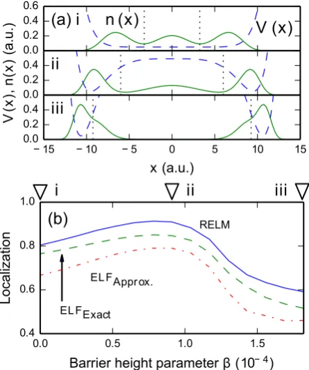
A constant value of α= 5×10−11 _{a.u. was used, while the value ofβ was varied: when} β = 0 there is no barrier in the potential, and as it is increased the height of the barrier grows. Three examples of the potentials and densities for different values ofβare shown in Fig. 1. This family of wells is interesting as the double-well potential only provides two natural sites for the three electrons to occupy.

0.0 0.2 0.4 0.6

(a) i n (x) _{V (x)}

0.0 0.2 0.4

V

(x

),

n

(x

)

(a

.u

.)

ii

−15 −10 −5 0 5 10 15

x (a.u.)

0.0 0.2 0.4 iii

0.0 0.5 1.0 1.5

Barrier height parameterβ(10−4₎

0.4 0.6 0.8 1.0

L

o

ca

liza

ti

o

n

EL FApprox.

RELM

EL FExact

i i iii

(b)

i ii iii

Figure 1. 3-electron double wells — (a) Plots of the external potentials (dashed blue) of three selected wells as the barrier height is increased. The ground-state charge densities (solid green) of these potentials are shown. The localisation regions used in the RELM calculations are also shown (dotted black); each contains exactly one electron’s worth of charge. (b) The localisation of the family of potentials, calculated using the three methods introduced – RELM, exact average ELF and approximate average ELF. All three measures agree how the barrier influences localisation. Triangles indicate the values ofβ for which the potentials are plotted in (a).

the barrier region owing to the Coulomb repulsion, as its height increases in (i) to (ii). As the presence of the barrier disperses the central electron across the system, it also drives the outer electrons toward the boundaries of the system, acting to increase the localisation of the system rather than decrease it (see Fig. 1(b)). As the strength of the barrier is increased further, it becomes energetically favourable for the central electron to move into the two side wells, as in (iii), reducing localisation.

In Fig. 1(b), the three measures agree on how the localisation of this family of potentials varies. The similarity between RELM and the exact average ELF is striking as the two methods are based on different mathematical interpretations of localisation: RELM is scaled probabilistically and ELF is scaled with respect to the HEG as reference. ApproximatingDσ does lead to a systematic lowering of the calculatedhELFi, but still yields the correct trend across the range of localisations calculated.

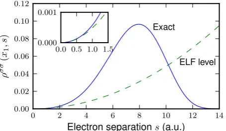
We next investigate the information contained in Dσ in more detail. Fig. 2 shows an example plot for a two electron system (specified in the caption), demonstrating the approximation made in Eq. 3 in practice. The conditional probability ρσσ

for a chosen value of r. As demanded by the Pauli exclusion principle, the probability of finding a second electron at the same position (s = 0) is zero. The function then shows a peak at the most likely separation the second electron is found at (we would normally expect as many peaks as there are remaining electrons in the system).

0 2 4 6 8 10 12 14

Electron separations(a.u.) 0.00

0.02 0.04 0.06 0.08 0.10 0.12

ρ

σ

σ

(

x1

,s

) Exact

ELF level

0.0 0.5 1.0 1.5 0.000

0.001

Figure 2. A plot of the conditional probability ρσσ

Cond(x1, s) against electron separationswherex1is fixed at the density maximum (2.64 a.u.) for the two-electron ground state of the potential of Fig.1(a)(i). The conditional probability (blue solid) is plotted with the ELF level approximation to it (green dashed). Insert: magnification of shortsbehaviour. Dσ does not contain any long range information and only correctly characterises short distances, in this example only∼0.6 a.u. Our strong ELF results suggest that this neglected long-range behaviour is not important for localisation.

Also shown on the plot is the approximated version of this conditional probability that is used in ELF calculations. As shown in Eq. 3, the ELF approximates this conditional probability as Dσ(r)s2_{/d and this is shown in the plot where Dσ has been}

calculated using Eq. 4. As shown in the inset in Fig. 2, this approximation is only effective over very short electron separations. RELM calculations use information over all s, so the agreement between our ELF and RELM calculations suggests that this longer-range s behaviour is not an important ingredient for a localisation measure to contain.

3.3. Time-dependent localisation

Next we look at a dependent system. As first derived by Dobson [20], in the time-dependent regime the approximate ELF is modified by the addition of an extra term to Eq. 6, producing the time-dependent ELF (TDELF) [21]. This equation becomes

Dσ≈

Nσ

X

i

|∇φσ

i| 2

− 1

4

|∇nσ|2

nσ −

jσ2

nσ, (8)

where jσ is the current density.

wavefunction of the well. Then at timet= 0 we apply a strong uniform d.c. electric field (potential −0.1x), driving the electrons strongly towards the right-hand well, causing them to “collide”. We also look at the non-interacting system with Pauli exclusion but no Coulomb interaction. We note that Coulomb interaction enhances localisation, and if the interaction strength is artificially enhanced the system is driven towards total localisation (RELM=1).

0.0 0.2 0.4 0.6 0.8 1.0

L o ca liza ti o n ELFExact e Sep. RELM (a)

0 10 20 30 40 50 60 70 80 Time (a.u.)

0.0 0.2 0.4 0.6 0.8 L o ca liza ti o n (b) 2 4 6 8 10 12 E le ct ro n se p a ra ti o n (a .u .) 2 4 6 8 10 E le ct ro n se p a ra ti o n (a .u .)

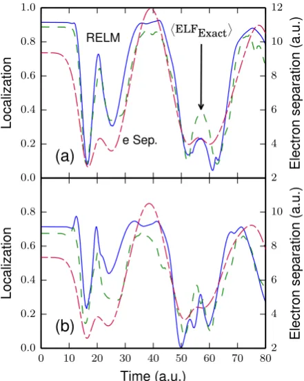
Figure 3. Localisation measures as a function of time for two electrons in the perturbedx10

well of Fig.1(a)(i). (a) The interacting system. RELM (solid blue) and exact average ELF (dashed green) continue to show good agreement. The expectation value of the electron separation (long dashed red) is also shown on the second axis and shows similar features. (b) The same plot for the non-interacting system. The behaviour of the system is similar, showing that Pauli exclusion is the main driver of localisation. RELM and ELF differ more significantly

Fig. 3 (a) shows how the localisation of the interacting electrons changes during the 80 a.u. of the simulation. Broadly, these results show strong changes in localisation over time. This is in contrast to the notion that localisation is a persistent characteristic of a system.

0.0 0.2 0.4 0.6 0.8 1.0

L o ca liza ti o n D ELFApprox.E D TDELFApprox.E RELM(KS) (a)

0 2 4 6 8 10 12 14

Time (a.u.) 0.0

0.2 0.4 0.6 0.8 L o ca liza ti o n (b) 2 4 6 8 10 12 E le ct ro n se p a ra ti o n (a .u .) 2 4 6 8 10 E le ct ro n se p a ra ti o n (a .u .)

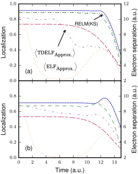
Figure 4. The curves in Fig. 3 for a shorter time interval, with the addition of approximate-ELF calculations based on the exact KS potential. For the interacting system in (a), the average approximate TDELF (dotted-dashed purple) and the GS approximate ELF (dotted orange) both delocalise the electrons too soon. If RELM is calculated from a KS Slater determinant (dotted black) its value is slightly underestimated. The TDELF, though an improvement on the original approximation, has a large spurious drop in localisation around t = 5 a.u. As shown in (b), this approximation performs better without interaction as the problematic drop is weaker. Without interaction, calculating RELM from a KS Slater determinant is exact and the two RELM curves coincide.

Fig. 3(b) shows the calculation repeated with no Coulomb interaction. The behaviour is broadly similar, but interaction seems to exaggerate some features and suppresses others. This comparison strengthens the argument that Pauli exclusion is the main driver of localisation.

Again, for both plots RELM and exact ELF show the same trends, although both measures show some unique features. The close agreement between the two measures still holds in a time-dependent context. We also note the agreement between exact ELF and RELM is reduced when the Coulomb interaction is turned off.

performs very poorly and for most of the calculation shows the system as erroneously delocalised. The extra current term in the TDELF makes a significant improvement. At around 5 a.u., however, it too shows an unphysical drop in localisation which analysis shows to occur in the left-hand well, predominantly associated with a large increase of the first term of Eq.8in the left half of the system which is not compensated for by the other terms. Instead, the real system delocalises both electrons at 12 a.u., later in the simulation. Clearly, the TDELF’s ignorance of correlation (beyond Pauli exclusion) in the wavefunction is limiting its description of localisation.

The approximate TDELF performs better when there is no electron-electron interaction [Fig. 4(b)]. It still shows a slow drop when the localisation is staying constant, but this erroneous drop is significantly weaker.

Additionally, we calculate RELM from a Slater determinant of the KS orbitals, the wavefunction of the fictitious non-interacting KS electrons. The strong correspondence again demonstrates that Pauli exclusion is the main driver of localisation. This approximation is exact when there is no electron interaction, but is slightly weaker when the electrons are interacting. This approximation is more successful than the approximate ELF calculations, which assume that the KS orbitals obey the HF equations.

One failure of the present approximation, concealed in the definition of ELF, is that it is not positive definite, leading to non-physical negative values of Dσ. If these values are set to zero, a small improvement in accuracy is achieved. Negative values should serve as a warning that the method is not performing reliably ¶.

4. Conclusions

We have studied electron localisation, which provides insight into important aspects of many-electron correlation, using a variety of measures across a range of ground-state and time-dependent systems. Our results show the strength of the ELF approach, despite its focus on short range exclusion. We further find that the usual approximate ELF provides good results for a range of ground-state systems, notwithstanding its simplicity and neglect of correlation, allowing the extraction of physical meaning from a simple measure based on one-electron wavefunctions. In contrast, time-dependent systems can often become surprisingly delocalised as electrons collide with one another, and in this case the simple approximate ELF is no longer adequate. When many-electron excited states are being strongly explored, improved approximate localisation measures are required.

5. Acknowledgements

We acknowledge funding from EPSRC, and thank David Tozer for helpful discussions.

[1] P Hohenberg and W Kohn. Inhomogeneous electron gas. Phys. Rev., 136(3B):B864, 1964. [2] W Kohn and LJ Sham. Self-consistent equations including exchange and correlation effects. Phys.

Rev., 140:A1133–A1138, Nov 1965.

[3] AD Becke and KE Edgecombe. A simple measure of electron localization in atomic and molecular systems. J. Chem. Phys., 92(9):5397–5403, 1990.

[4] A Savin, R Nesper, S Wengert, and TF F¨assler. ELF: The electron localization function. Angew.

Chem., Int. Ed., 36(17):1808–1832, 1997.

[5] JF Dobson. Interpretation of the Fermi hole curvature. J. Chem. Phys., 94(6):4328–4333, 1991. [6] B Silvi and A Savin. Classification of chemical bonds based on topological analysis of electron

localization functions. Nature, 371(6499):683–686, 1994.

[7] MJP Hodgson, JD Ramsden, TR Durrant, and RW Godby. Role of electron localization in density functionals. Phys. Rev. B, 90(24):241107, 2014.

[8] W Kohn and AE Mattsson. Edge electron gas. Phys. Rev. Lett., 81(16):3487, 1998.

[9] F Hao, R Armiento, and AE Mattsson. Using the electron localization function to correct for confinement physics in semi-local density functional theory. J. Chem. Phys., 140(18):18A536, 2014.

[10] J Sun, A Ruzsinszky, and JP Perdew. Strongly constrained and appropriately normed semilocal density functional. Phys. Rev. Lett., 115:036402, Jul 2015.

[11] P Mori-S´anchez, AJ Cohen, and W Yang. Localization and delocalization errors in density functional theory and implications for band-gap prediction. Phys. Rev. Lett., 100:146401, Apr 2008.

[12] MJP Hodgson, JD Ramsden, and RW Godby. Origin of static and dynamic steps in exact Kohn-Sham potentials. Phys. Rev. B, 93:155146, Apr 2016.

[13] A Savin, O Jepsen, J Flad, OK Andersen, H Preuss, and HG von Schnering. Electron localization in solid-state structures of the elements: the diamond structure. Angew. Chem., Int. Ed., 31(2):187–188, 1992.

[14] E Matito, B Silvi, M Duran, and M Sol`a. Electron localization function at the correlated level.

J. Chem. Phys., 125(2):024301, 2006.

[15] MJP Hodgson, JD Ramsden, JBJ Chapman, P Lillystone, and RW Godby. Exact time-dependent density-functional potentials for strongly correlated tunneling electrons. Phys. Rev. B, 88(24):241102, 2013.

[16] S K¨ummel and L Kronik. Orbital-dependent density functionals: Theory and applications. Rev.

Mod. Phys., 80(1):3, 2008.

[17] AJ Cohen, P Mori-S´anchez, and W Yang. Insights into current limitations of density functional theory. Science, 321(5890):792–794, 2008.

[18] E R¨as¨anen, A Castro, and EKU Gross. Electron localization function for two-dimensional systems.

Phys. Rev. B, 77(11):115108, 2008.

[19] M Erdmann, EKU Gross, and V Engel. Time-dependent electron localization functions for coupled nuclear-electronic motion. J. Chem. Phys., 121(19):9666–9670, 2004.

[20] JF Dobson. Alternative expressions for the Fermi hole curvature. J. Chem. Phys., 98(11):8870– 8872, 1993.

[21] T Burnus, MAL Marques, and EKU Gross. Time-dependent electron localization function. Phys.