An Enhanced Bailout Protocol for Mixed Criticality Embedded Software

White Rose Research Online URL for this paper:

http://eprints.whiterose.ac.uk/102518/

Version: Accepted Version

Article:

Bate, Iain John orcid.org/0000-0003-2415-8219, Burns, Alan

orcid.org/0000-0001-5621-8816 and Davis, Robert Ian orcid.org/0000-0002-5772-0928

(2017) An Enhanced Bailout Protocol for Mixed Criticality Embedded Software. IEEE

Transactions on Software Engineering. ISSN 0098-5589

https://doi.org/10.1109/TSE.2016.2592907

[email protected] https://eprints.whiterose.ac.uk/ Reuse

Items deposited in White Rose Research Online are protected by copyright, with all rights reserved unless indicated otherwise. They may be downloaded and/or printed for private study, or other acts as permitted by national copyright laws. The publisher or other rights holders may allow further reproduction and re-use of the full text version. This is indicated by the licence information on the White Rose Research Online record for the item.

Takedown

If you consider content in White Rose Research Online to be in breach of UK law, please notify us by

An Enhanced Bailout Protocol for Mixed

Criticality Embedded Software

Iain Bate

1

_{, Alan Burns}

1

_{and Robert I. Davis}

1,2

1

_{Department of Computer Science, University of York, York, UK}

2

_{INRIA, France}

{

iain.bate, alan.burns, rob.davis

}

@york.ac.uk

Abstract—To move mixed criticality research into industrial practice requires models whose run-time behaviour is acceptable to systems engineers. Certain aspects of current models, such as abandoning lower criticality tasks when certain situations arise, do not give the robustness required in application domains such as the automotive and aerospace industries. In this paper a new bailout protocol is developed that still guarantees high criticality software but minimises the negative impact on lower criticality software via a timely return to normal operation. We show how the bailout protocol can be integrated with existing techniques, utilising both offline slack and online gain-time to further improve performance. Static analysis is provided for schedulability guarantees, while scenario-based evaluation via simulation is used to explore the effectiveness of the protocol.

Index Terms—Real-Time Systems, Mixed Criticality, Fixed Priority Scheduling, Mode Changes.

F

Preliminary publication

This paper extends initial research into a bailout protocol for mixed criticality systems presented at ECRTS 2015 [1]. The additional material includes: An extended worked example illustrating, in figures 1 and 2, the behaviour of the bailout protocol as compared to the baseline Adaptive Mixed Criticality (AMC) scheduling policy. Extensions to reclaim gain-time, which becomes available when a task executes for less than its worst-case execution time budget. Integration of this technique with the bailout protocol is described in Section 5. An extended scenario based evaluation, in Section 6. This examines the benefits of gain-time reclamation in conjunction with the baseline Adaptive Mixed Criticality (AMC) scheduling policy and with the bailout protocol. The evaluation also covers additional metrics including the number of times that the system has to go into a HI-criticality mode, and the amount of time spent in that mode. It is also extended to show how a variety of different factors impact the performance of the bailout protocol and other scheduling policies, thus showing the broad range of circumstances in which the protocol is effective. Finally, in Section 8 we show how the bailout protocol can be adapted to systems with multiple criticality levels.

1

I

NTRODUCTION

A

Nincreasingly important trend in the design of real-time and embedded software systems is the integration of components with different levels of criticality onto a common hardware platform. Criticality is a designation of the level of assurance against failure needed for a system component, where the level of assurance needed depends on both the likelihood of failure and the consequences of that failure [2]. A mixed criticality system (MCS) is one that has two or more distinct levels (for example safety critical and mission critical). Perhaps up to five levels may be identified. Most of the complex embedded systems found in, for example, the automotive and avionics industries are evolving into

integrated rather than federated mixed criticality systems in order to meet stringent non-functional requirements relating to cost, space, weight, heat generation and power consumption; the latter being of particular relevance to mobile systems.

The fundamental research question underlying these initiatives and standards is: how, in a disciplined way, to reconcile the conflicting requirements ofpartitioningfor assurance andsharing

for efficient resource usage. This question gives rise to theoretical problems in modeling and verification, and systems problems relating to the design and implementation of the necessary hardware and software run-time controls.

Although the formal study of mixed criticality systems is a relatively new endeavour, starting with the paper by Vestal [3], a standard model has emerged (see for example [4]–[9]). For dual criticality systems (with the two levels: HI-criticality and LO-criticality) this standard model has the following properties:

• _{A mixed criticality system is defined to execute in one of two} modes: anormalmode and aHI-criticalitymode.

• _{All software is structured as concurrently executingtasksthat} are scheduled by a dependable RTOS (Real-Time Operating System) supporting fixed priority preemptive scheduling. • Each task is characterised by its criticality level (e.g. HI- or

LO-criticality), the minimum inter-arrival time of its jobs (period denoted byT), deadline (relative to the release of each job, denoted byD) and worst-case execution time (one per criticality level up to the criticality level of the task), denoted byC(HI)andC(LO). A key aspect of the standard MCS model is thatC(HI)≥C(LO)[3].

• _{The system starts in the normal mode, and remains in that} mode as long as all jobs execute within their LO-criticality execution times (C(LO)).

• _{If any HI-criticality job executes for its}C(LO)_{execution time} without completing then the system immediately degrades to the HI-criticality mode.

time without completing then that job is immediately aborted by a runtime monitoring mechanism.

• As the system moves to the HI-criticality mode all LO-criticality tasks are abandoned. No further LO-criticality jobs are executed.

• The system remains in the HI-criticality mode.

The movement from normal mode to HI-criticality mode is a form of graceful degradation. Following a timing anomaly only the HI-criticality tasks are guaranteed to meet their deadlines.

The motivation for the standard model having two values for the Worst-Case Execution Time (WCET) [3], [10] is taken from either of two situations often seen in industrial practice [11]. The first situation involves the High WaterMark (HWM), i.e. the largest execution time observed during testing, which is highly reliable as testing for functional correctness is intensive (e.g. MCDC coverage). This value would be taken asC(LO). However for the most critical software an engineered safety margin is added to give aC(HI)

value. Values for this engineered safety margin come from industrial practice and are based on engineering judgement and experience. A margin of around 20% is typical in aerospace applications1_{[12]. It} is considered sufficiently unlikely that this value will be exceeded2_. The second situation is when static or hybrid analysis is used to obtain a WCET, which can be treated asC(HI). Even though this value is considered sound [11], it is often too pessimistic, and its use may lead to difficulties in obtaining a schedulable system. Again the HWM may be used as C(LO). In both cases, it is necessary that the system is schedulable when all tasks execute for

C(LO); however it is also important to gracefully degrade when

C(LO)is exceeded, i.e. HI-criticality tasks must still meet their deadlines and as few as possible of the LO-criticality tasks miss their deadlines.

The abstract behavioural model described above has been useful in allowing key properties of mixed criticality systems to be derived, but it is open to criticism from systems engineers that it does not match their expectations [2]. In particular:

• In the HI-criticality mode LO-criticality tasks should not be abandoned. Some level of service should be maintained if at all possible, as LO-criticality tasks are still critical.

• It should be possible for the system to return to the normal mode as soon as conditions are appropriate. In this mode all functionality should be provided.

Clearly, in general, if the system is in the HI-criticality mode and all HI-criticality tasks are executing for the maximum time defined for such tasks then the LO-criticality tasks will not be able to receive enough execution time to guarantee that their deadlines are met. However, in many situations the worst-case conditions will not be experienced and in this case LO-criticality tasks should receive some level of service.

The main contribution of this paper is the introduction of the

Bailout Protocolin which HI-criticality tasks are not allowed to fail (they are too important to fail) and therefore LO-criticality tasks must sacrifice their quality of service by not starting a certain number of jobs. The actual number of sacrificed jobs depends on the size of the bailout and the time needed for recovery. However, once the bailout has been serviced the LO-criticality tasks can return to their full timely behaviour. While the bailout protocol

1. Note, we know of no theoretical support for using such a value, rather such margins come from engineering experience.

2. In some systems, further runtime monitoring may be employed to ensure that such overruns, however unlikely, do not lead to significant system failure.

allows LO-criticality jobs to be dropped, rather than abandon jobs that have been released, and so waste the consumed execution time and potentially leave them in an inconsistent state, it allows these jobs to continue. However, it disables the release of new jobs of LO-criticality tasks until the system is back in the normal mode of execution whereby it can again guarantee all tasks. (Note many forms of analysis actually reduce their complexity by assuming all released jobs will complete). The bailout protocol aims to restore the normal mode as soon as possible following an interval of HI-criticality only activity, and so minimise the number of LO-criticality jobs that miss their deadlines or are not executed. The bailout protocol thus reduces the amount of time spent in the HI-criticality mode. In addition, we show how the protocol can be complemented by techniques based on gain-time reclamation [13] and slack stealing [14], [15] to further reduce both the number of times the system enters HI-criticality mode and the amount of time that it spends in that mode.

To comply with the requirements of MCS, scheduling policies and protocols must ensure that HI-criticality tasks always meet their deadlines, and that all tasks meet their deadlines when the system is in normal mode. Schedulability analysis provides the answers to these questions. Beyond such compliance, the relative effectiveness of the different protocols is judged on the basis of criteria such as the number of times the system enters the HI-criticality mode, the amount of time spent in that mode, and the number of LO-criticality jobs that either miss their deadlines or are abandoned. Scenario-based assessment using large-scale simulations provides information about these metrics although the results obtained are only valid for the range of scenarios explored.

The remainder of the paper is organised as follows. In Section 2, we discuss related work, introduce the formal system model used in this paper, and recapitulate on the basic schedulability analysis for MCS which we build upon. Approaches to degraded service are considered in Section 3. In Section 4, we define the

bailout protocolfor MCSs, and in Section 5 show how it can be integrated with techniques that make use of spare capacity that is either available both off-line, or becomes available at runtime, to improve performance. A key aspect of this paper is the evaluation of MCS protocols via scenario-based simulation; this is addressed in Section 6. Analysis for the bailout protocol is given in Section 7. An extension of the protocol to more than two criticality levels is outlined in Section 8. Finally, Section 9 concludes with a summary and a discussion of future work.

2

B

ACKGROUND

Background material on MCS research can be obtained from the following sources [3]–[6], [8], [16]–[18]. An ongoing survey of MCS research by [10] is available from the MCC (Mixed Criticality Systems on Many-core Platforms) project website3_{. We} note that while mixed criticality behaviour has some similarities to traditional mode changes, there are also significant differences [2], [19]. These include the mode change being driven by a particular temporal rather than functional behaviour, permitting a more specific schedulability analysis.

2.1 System Model and Assumptions

In this paper, we are interested in the Fixed Priority Preemptive Scheduling (FPPS) of a mixed criticality system comprising a static

set ofnsporadic tasks which execute on a single processor. We assume without loss of generality that each taskτi has a unique

priority, given by its index. Thus taskτ1has the highest priority and taskτnthe lowest. We assume a discrete time model in which

all task parameters are given as integers. Each task,τi, is defined

by its period (or minimum arrival interval), relative deadline, worst-case execution time, and level of criticality (defined by the system engineer responsible for the entire system): (Ti,Di,Ci,Li). We

restrict our attention to constrained-deadline systems in which

Di ≤Tifor all tasks. Further, we assume that the processor is the

only resource that is shared by the tasks, and that the overheads due to the operation of the scheduler and context switch costs can be bounded by a constant, and hence included within the worst-case execution times attributed to each task.

In a mixed criticality system, further information is needed in order to undertake schedulability analysis. In general a task is defined by: (T,D,C~,L), whereC~ is a vector of values – one per criticality level, with the constraintL1> L2⇒C(L1)≥C(L2)

for any two criticality levelsL1 and L2. In this paper we are mainly concerned with dual criticality systems, with criticality levels LO and HI (where LO <HI). Thus each LO-criticality task has a single worst-case execution time estimateC(LO), while each HI-criticality task has two worst-case execution time estimates

C(LO)andC(HI)withC(HI)≥C(LO).

2.2 Current Scheduling Analysis and its Limitations

Although the standard model of mixed criticality system behaviour requires an immediate change to the HI-criticality mode and the consequential abandonment of all active LO-criticality jobs, the analysis of this model has shown [16], [20], [21] that the mixed criticality schedulability problem is strongly NP-hard even if there are only two criticality levels. Hence only sufficient rather than exact analysis is possible. One of the consequences of this constraint is that a significant proportion of the available analyses that have been produced for MCSs actually assume that any LO-criticality job that has been released by the time of the mode change will complete, rather than being aborted.

For example, the Adaptive Mixed Criticality (AMC Method 1 or AMC-rtb) approach presented at RTSS by [5] first computes the worst-case response times for all tasks in the normal mode (denoted byR(LO)). This is accomplished by solving, via fixed point iteration, the following response-time equation for each task

τi:

Ri(LO) = Ci(LO) + X

∀j∈hp(i)

_R i(LO)

Tj

Cj(LO) (1)

wherehp(i)is the set of all tasks with priority higher than that of taskτi.

During the criticality change the only concern is HI-criticality tasks, for these tasks:

Ri(HI) = Ci(HI) +

X

∀j∈hpH(i)

_R i(HI)

Tj

Cj(HI)

+ X

∀k∈hpL(i)

_R i(LO)

Tk

Ck(LO) (2)

wherehpH(i)is the set of HI-criticality tasks with priority higher than that of taskτi andhpL(i)is the set of LO-criticality tasks

with priority higher than that of task τi. Sohp(i)is the union

of hpH(i)and hpL(i). Note Ri(HI) is only defined for

HI-criticality tasks.

This equation takes into account the fact that LO-criticality tasks cannot execute for the entire busy period of a HI-criticality task in the HI-criticality mode. A change to the HI-criticality mode must occur at or beforeRi(LO)which caps the interference from

LO-criticality tasks asRi(HI)must be greater thanRi(LO).

The cap is however at the maximum possible level. The maximum number of LO-criticality jobs are assumed to interfere and each of these jobs is assumed to complete – each inducing the maximum interference of Ck(LO). Note that if, for any

HI-criticality task, Ri(HI) ≤ Di during the transition to the

HI-criticality mode then the task will remain schedulable once the HI-criticality mode is fully established and there is no interference from LO-criticality tasks.

This AMC approach assumes that once the system goes into the HI-criticality mode then it will stay in that mode. As discussed in the introduction this is not an acceptable behaviour in practice. A simple but necessary extension to AMC is therefore to allow a switch back to the normal mode when the system experiences an

idle instant4_{. This is a well-known protocol for controlling mode} changes [22]. In this paper we will refer to this extended approach as AMC+.

In the remainder of this paper, for AMC and AMC+, we assume that any job of a LO-criticality task that is released before HI-criticality mode is entered may complete its execution, since this is allowed by the analysis; however, LO-criticality jobs released during HI-criticality mode are abandoned by these schemes.

3

D

EGRADED

S

ERVICE FOR

LO-C

RITICALITY

T

ASKS

The key properties of MCS scheduling are (i) that if all tasks execute within theirC(LO)bounds then all deadlines for all task will be satisfied, and (ii) that HI-criticality tasks will always meet their deadlines.

Notwithstanding these key static properties of a system, an actual implementation must exhibit clear and effective behaviours for all of its potential run-time characteristics. In particular, for a dual criticality system, if at some point during its execution only the HI-criticality jobs can be guaranteed, then what level of service can be expected for the LO-criticality jobs? As indicated in the introduction it is not acceptable to permanently abandon these tasks just because they cannot be fully guaranteed.

The dual requirement (both to meet all deadlines and to have sensible behaviour when deadlines are missed) is not a contradiction, rather it is a necessary property of any robust system model. MCSs have, in this regard, a number of similarities to fault tolerance systems: faults should be avoided, but also faults should be tolerated and result in minimum disturbance to the system [19].

Various forms of degraded service have been proposed for LO-criticality tasks in the literature: Run all tasks, but extend their periods and/or deadlines – sometimes called the elastic task model [23]. Run all tasks but reduce the executions times of LO-criticality tasks (i.e.C(HI) ≤ C(LO)for these tasks) [24] – perhaps by switching to simpler version of the software. Drop jobs from a specific subset of tasks [25], [26] or skipsi in everymi

jobs of each task [27].

In comparison with the bailout protocol presented in this paper, the above methods prescribe specific changes to the behaviour of LO-criticality tasks either increases in their periods, decreases in their execution times (and hence the need for different versions of the software), or dropping specific jobs e.g. 1 job in every 3. The bailout protocol on the other hand does not change the primary behaviour of LO-criticality tasks, but rather focuses on re-instating them fully as quickly as possible. This has less impact on overall schedulability, since similar to AMC, there are no guarantees for LO-criticality tasks in the HI-criticality / bailout mode. In systems where transitions to HI-criticality mode are rare, and some missed jobs of LO-criticality tasks can be tolerated, then the bailout protocol may provide an effective solution. In systems where LO-criticality tasks must continue to provide some level of guaranteed service even when the system is in its degraded mode, then other methods need to be used.

We note that the approach taken by the bailout protocol is orthogonal to those of job dropping [26] and weakly-hard guarantees for LO-criticality tasks proposed in [27], hence it is possible that the different techniques could be combined; such work is however beyond the scope of this paper.

An orthogonal approach to improving the overall service for LO-criticality tasks was adopted by Santy et al. [7]. They effectively scale theC(LO)values using sensitivity analysis until the system is just schedulable. Using these values at runtime makes the system more robust, since LO-criticality tasks can execute for longer, and HI-criticality tasks are less likely to exceed their larger budgetedC(LO)values, making the system less likely to enter its HI-criticality mode. This approach was subsequently refined by Burns and Baruah [24] using Robust Priority Assignment techniques [28] that permit priorities to change during the sensitivity analysis process.

A further important aspect of providing service for LO-criticality tasks is the ability to restore the system to its normal mode following an interval of HI-criticality behaviour. As mentioned previously, this can be achieved by waiting for an idle instant. Santy et al. [7] explored this approach, and also developed a protocol for multiprocessor scheduling where there may be no idle instant across all processors [29]. Further work by Ren et al. [30] focused on partitioned multiprocessor scheduling. Here, each HI-criticality task is associated with a group of LO-criticality tasks. Thus the overrun of the HI-criticality task can only impinge on the execution of LO-criticality tasks in the same task group. Task groups are scheduled according to EDF, with servers used within each group to ensure mixed criticality guarantees.

4

T

HE

B

AILOUT

P

ROTOCOL

We now describe the Bailout Protocol assuming two levels of criticality in the system software.

4.1 Protocol, modes, and mechanisms

At run-time, dual criticality systems are typically defined to be in one of two modes:normal modeandHI-criticality mode; however, these terms can be confusing. With the bailout protocol, we defined three modes: normal mode, bailout mode and recovery mode. Normal mode is as defined above. Bailout and recovery modes correspond to the traditional HI-criticality mode.

The bailout protocol comprises the following modes and mechanisms, which operate only in the mode for which they are described.

In all modes, LO-criticality tasks are prevented from executing for more than theirC(LO)values. LO-criticality tasks dispatched in normal mode, continue to execute in both bailout and recovery modes. (Note, such jobs may miss their deadlines in these modes, but continue to execute provided they do not exceedC(LO)).

Normal mode:

(i) While all jobs of HI-criticality tasks execute for no more than theirC(LO)values, then the system remains in normal mode. (ii) If any HI-criticality job executes for its C(LO) value without signalling completion it must take out a loan ofC(HI)−

C(LO); this loan is always granted, and the system moves into the bailout mode. The bailout fund (BF) is initialised toBF =

C(HI)−C(LO).

Bailout mode:

(iii) If any HI-criticality job executes for its C(LO) value without signalling completion then it must also take out a loan ofC(HI)−C(LO), adding to the bailout fund:BF =BF+

C(HI)−C(LO).

(iv) If any HI-criticality job completes with an execution time ofe, with e ≤ C(LO)then it donates its underspend (if any), reducing the bailout fund:BF =BF−(C(LO)−e).

(v) If any LO-criticality job completes with an execution time ofe, withe≤C(LO)then it donates its underspend (if any) to the bailout fund:BF =BF −(C(LO)−e). Note, such a job would need to have been released in an earlier normal mode.

(vi) If any HI-criticality job with a loan completes with an execution time ofe, withC(LO)< e≤C(HI)then it donates its loan underspend, reducing the bailout fund: BF = BF −

(C(HI)−e).

(vii) LO-criticality jobs released in bailout mode are abandoned (not started). Further, when the scheduler would otherwise dispatched such a job, the job’s budget ofC(LO)is donated to the bailout fund:BF =BF−C(LO).

(viii) If the bailout fund becomes zero (noteBFis constrained to never become negative), then the lowest priority HI-criticality job with outstanding execution is recorded (let this job beJk) and

the recovery mode is entered5_.

(ix) If during bailout mode, an idle instant occurs, then an immediate transition is made to normal mode, andBFis reset to zero6.

Recovery mode:

(x) LO-criticality jobs released in recovery mode are abandoned (not started).

(xi) If any HI-criticality job executes for its C(LO) value without signalling completion, then the system re-enters bailout mode – as described in (ii) above.

(xii) When the jobJknoted at the point when recovery mode

was last entered completes, then the system transitions to normal mode.

The bailout protocol is designed to have a simple implementation, with each operation (i) to (xii) amounting to only a few instructions, requiring onlyO(1)time, and incorporated into existing RTOS code for context switching or execution time budget monitoring. All actions take place at the release or

5. JobJkdefines the extent of the recovery mode, which is necessary to ensure that no HI-criticality job can be subject to more interference than accounted for by the analysis of AMC, for further details see Theorem 7.4 in Section 7 and the discussion that follows it.

completion of a job, which are well defined RTOS operations in FPPS, or when a job executes for C(LO) without signalling completion. In the case of a LO-criticality task, the action required in the latter case corresponds to execution time budget enforcement, as needed in any high integrity implementation whether AMC or the bailout protocol were being employed or not. Such an overrun may be detected via a timer interrupt and the job aborted. In the case of a HI-criticality job executing forC(LO)

without signalling completion, then the action required is to change to HI-criticality mode, preventing further releases of LO-criticality jobs. Since the HI-criticality job continues to execute, such a mode change may be soundly deferred until the next scheduling point (i.e. job release or completion), and so no timer interrupt is required; rather only execution time monitoring is needed. (This is the case with both AMC and the bailout protocol). We note that the bailout protocol does not change task priorities, nor introduce any additional context switches which are not also present under basic FPPS.

4.2 Example

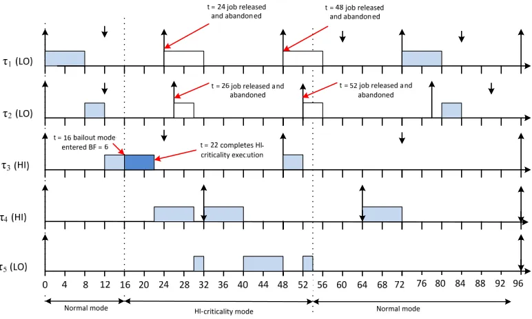
We now give an example illustrating the behaviour of the bailout protocol. This example includes five tasks:τ1,τ2, andτ5are LO-criticality tasks, whileτ3andτ4are HI-criticality. Taskτ1has the highest priority and taskτ4the lowest. The parameters of the tasks are given in table 1 below. The tasks are schedulable according to the AMC-rtb schedulability test with theR(LO)andR(HI)

upper bounds on the worst-case response times given in the table.

TABLE 1 Example task parameters

τi L Ci(LO) Ci(HI) Ti Di R(LO) R(HI)

τ1 LO 8 - 24 12 8

-τ2 LO 4 - 26 12 12

-τ3 HI 4 10 48 24 16 22

τ4 HI 8 8 32 32 24 30

τ5 LO 12 - 92 92 92

-Figure 1 illustrates the behaviour of the bailout protocol. At timet= 16, taskτ3has executed forC(LO)without signalling completion, hence bailout mode is entered. AsC(HI) = 10,BF

is initialised to 6 (sinceC(LO) = 4). Taskτ3completes its HI-criticality execution at timet= 22; however, the system cannot simply resume normal mode behaviour, since then the releases of taskτ1andτ2att= 24andt= 26respectively would result in taskτ4(HI-criticality) missing its deadline. Instead, sinceBF >0, the system remains in bailout mode. At timet= 24the second job of taskτ1is released; however, as the system is in bailout mode, and the task is of LO-criticality, then the job is abandoned at the time it would have started to execute (t= 24in this case) repaying the bailout fund, which now goes to zero. However, the system still cannot resume normal mode operation, as doing so would result in taskτ4(HI-criticality) missing its deadline due to interference from the second job of taskτ2. Instead the system enters recovery mode and records the lowest priority HI-criticality job with outstanding execution. This is the first job of taskτ4. When this job completes att= 30, the system re-enters normal mode. It is interesting to note that in this example, if taskτ4were a LO-criticality task, then recovery mode would end immediately (i.e. at the same time as bailout mode att= 24), the second job of taskτ2would not be

abandoned, and taskτ4would miss its deadline. This shows that under the bailout protocol, (in common with AMC) LO-criticality jobs with release times and deadlines that span some HI-criticality behaviour cannot be guaranteed to meet their deadlines, even if the system returns to normal behaviour before they complete.

We note that without the bailout protocol, this system would not revert to normal mode until an idle instant occurred, hence the third jobs of both tasksτ1andτ2would not be executed, and the system would not return to normal mode until timet = 54. This is illustrated in Figure 2 which shows the schedule for the same behaviour under AMC. This example serves to illustrate the advantages of the bailout protocol, fewer jobs LO-criticality jobs are dropped, and the system returns to normal mode 14 time units after the HI-criticality behaviour is detected, rather than 38 time units after.

4.3 Discussion

A more general comparison can also be made between the bailout protocol and AMC+. Recall that AMC+ relies on the simple idle-instantprotocol [22] to revert to normal mode. Since the bailout protocol also returns to normal mode on an idle instant (operation (ix) in bailout mode and potentially also operation (xii) in recovery mode), but can also make earlier transitions back to normal mode, it dominates AMC+ in terms of the time taken between entering HI-criticality / bailout mode and returning to normal mode. Stated otherwise, the bailout protocol takes no longer than AMC+ to return to normal mode, assuming the same initial pattern of task executions.

In the extreme case where all jobs take their maximum execution time (either C(LO) or C(HI)) then the interval needed to recover back to normal mode can still be no greater with the bailout protocol; it may however be shorter due to the bailout fund being reduced by the budgets of abandoned LO-criticality jobs (operation (vii) in the protocol). In the worst-case, when there are also no abandoned LO-criticality jobs to reduce the bailout fund, then the interval needed to recover back to normal mode is the same as that for AMC.

It is also interesting to consider, for a schedulable system, the longest possible time that may elapse between entering HI-criticality / bailout mode and the transition back to normal mode. This is the same for both the bailout protocol and AMC+. For a schedulable system, in the worst-case, both must wait for an idle instant. We now derive an upper bound A on the length of time that can elapse before such an idle instant occurs. We pessimistically assume the worst-case possible behaviour of both HI- and LO-criticality tasks. Each LO-criticality task may give rise to a single job which executes during the HI-criticality mode (such jobs must have been released just before the transition to the HI-criticality mode). In the case of the HI-criticality tasks, we assume (pessimistically) that at the transition each task has an outstanding job that has been delayed from executing for as long as possible and now requires itsC(HI)execution time before completing at its deadline. Subsequent jobs are then released as soon as possible also requiringC(HI). This scenario is captured by the following recurrence relation:

A= X

∀j∈aH

L+ (Dj−Cj(HI))

Tj

Cj(HI) + X

∀k∈aL

Ck(LO)

t = 16 bailout mode

entered BF = 6 t = 22 completes HI-criticality execution

Deadline met by virtue of recovery

mode

1(LO)

t = 24 job released and abandoned as system is in bailout mode Gives 8 to BF which is now zero

t = 26 job released and abandoned as system is in recovery mode

2(LO)

3(HI)

4(HI)

4 8 12 16 20 24 40 44 0 28 32 36

Normal mode Bailout mode Recovery mode

Normal mode

5(LO)

[image:7.612.89.476.53.287.2]

48 52 56 60 64 68 72 76 80 84 88 92 96

Fig. 1. Example showing the operation of the bailout protocol, including normal, bailout and recovery modes.

 

Fig. 2. Example showing the operation of AMC, including normal and HI-criticality modes.

whereaLis the set of all LO-criticality tasks, andaH is the set of all HI-criticality tasks. Iteration starts with an initial value ofA= P

∀j∈aHCj(HI) +P∀k∈aLCk(LO)and ends on convergence,

which is guaranteed since the utilization of HI-criticality tasks computed using theirC(HI)values cannot exceed 1.

Note, increasing execution time budgets, as discussed in the next section, may increase the maximum time required to return to normal mode due to the increase in LO-criticality execution which may take place after the transition to the HI-criticality mode. We note that while the system is guaranteed to return to LO-criticality mode after an interval of at most A. Such a guarantee is not particularly useful, since further HI-criticality behaviour may force an almost immediate return to the HI-criticality mode.

5

I

MPROVEMENTS

In this section we describe two methods, one offline and the other online, which are complementary to the bailout protocol. These methods help to reduce the number of times that a given system will go into bailout mode, and the amount of time that it spends in that mode, hence reducing the number of LO-criticality jobs that miss their deadlines or are abandoned.

5.1 Slack Time: Increasing Execution Time Budgets

[image:7.612.90.476.324.556.2]

to C(LO)values, can be changed without making the system unschedulable, effectively making use of the available slack in the system [33]. Intuitively, this method is compatible with the bailout protocol, since it effectively increases the execution time budgets, normally based onC(LO)values, while ensuring that the system remains provably schedulable. (Note, it is important here to distinguish between the worst-case execution time estimates e.g.

C(LO)obtained for the software, and the potentially larger values with a greater engineering margin, that can be used at runtime as execution time budgets).

The specific method we use is as follows: First, we increase the execution time budgets of all HI-criticality tasks as much as possible while ensuring that the system remains schedulable according to AMC-rtb analysis (i.e. (1) and (3)). We do this by forming a binary search for the largest value ofαsuch that the system remains schedulable when all HI-criticality task’sC(LO)

values are replaced byC(BU) =min(C(HI), αC(LO)). Note we useC(BU)rather thanC(LO)to emphasize that these are no longer the LO-criticality WCET estimates associated with those HI-criticality tasks, but ratherexecution time budgetsthat will be used to police normal mode behaviour at runtime. The initial lower value ofαused for the binary search is 1, since the system is assumed to be schedulable under AMC-rtb to begin with, and the initial upper value is given by the largestC(HI)/C(LO)for any HI-criticality task. At each step of the binary search, Audsley’s Optimal Priority Assignment algorithm [34] is used along with the single task schedulability test (i.e. (1) and (3)) to determine if the system is schedulable for that value ofα.

Second, we use a similar process to further increase, if possible, theC(BU)value for each individual task in turn, since after the first step, some but not all of the C(BU) values may still be increased without making the system unschedulable. (We do this for all HI-criticality tasks in order of increasing deadlines).

At runtime, we use FPPS along with the bailout protocol, replacing all occurrences ofC(LO)for HI-criticality tasks by the largerC(BU)values. We refer to the basic bailout protocol as BP, and the more sophisticated approach described here as BPS (Bailout Protocol with Sensitivity analysis). For systems that are schedulable under classical FPPS (i.e. assuming that all jobs may take an execution time that corresponds to their own criticality level i.e.C(HI)for HI-criticality tasks, andC(LO)for LO-criticality tasks), then BPS has the useful property, unlike AMC+ and BP, that no LO-criticality jobs miss their deadlines. This is the case, since for such systems the first step described above will result in C(BU) = C(HI) for all HI-criticality tasks. The AMC+ approach may also take advantage of increasedC(BU)values. We refer to such an approach as AMC+S.

We note that in practice, some of the statically available slack in the system could also be used to provide LO-criticality tasks with additional headroom for longer than expected execution, i.e. execution budgets larger thanC(LO).

5.2 Gain Time

Gain Time refers to the difference between the execution time actually used by a job and the execution time budget that it was allocated. We assume that jobs have an initial execution time budget given byc=C(BU), whereC(BU)is the execution budget for the task, eitherC(LO)or derived as described in section 5.1 above. At runtime, it is likely that many jobs will complete in less than their execution time budgets. A number of mechanisms exist that

can make this gain time available for use by other jobs [33], [35], [36], while ensuring that schedulability is unaffected.

The method we use comes from the Extended Priority Exchange algorithm [35] and operates in conjunction with the bailout protocol,

onlyin normal mode. In normal mode, whenever a job completes in an execution timee, which is less than its budget (i.e.e < c), then the gain timec−eis added to the execution time budget of the next lower priority active job (i.e. the next job in the run queue). This has no effect on schedulability, since the higher priority job (running first) could have legitimately executed for this gain time without any deadlines being missed. Passing gain time from one job to another in this way makes it less likely that jobs requiring more execution time than expected will actually exceed their execution time budgets, in turn making the system more robust to overruns (i.e. jobs exceedingC(LO)) and less likely to enter bailout mode. We denote this scheme as BPG and BPGS if static slack is used as well as gain time. We note that the gain time mechanism can be employed with AMC+ and AMC+S, in which case (unlike with the bailout protocol) it can operate in both normal and HI-criticality modes, but is only beneficial in the normal mode.

The gain time mechanism has a low overhead with O(1)

budget accounting at the completion of each job. This mechanism could potentially be improved by representing gain time in terms of the capacity of servers running at different priorities, with tasks, (including the idle task) first using spare capacity from the highest priority server with available capacity. Such an approach would better preserve any gain time generated. For example if the processor became idle, then spare capacity would not simply be discarded, but instead it would be gradually idled away, hence even after an idle period, tasks could still potentially benefit from previously generated gain time. Although theoretically superior, such an approach would require more complex runtime support than the standard mechanism which can be simply implemented by passing the remaining execution time budget at completion to the task at the head of the ready queue (the next task to run). In this paper, we therefore explore only the standard mechanism. We also note that in bailout mode, the gain time mechanism is not used, since the bailout protocol effectively makes use of gain time to hasten recovery.

6

S

CENARIO

-B

ASED

E

VALUATION

In this section, we present a scenario-based evaluation of the performance of the bailout protocol using an experimental framework / simulation. This is a commonly-used approach to evaluating real-time systems [37]–[39] when it is not practical to do effective ‘what-if’ analysis by other means. Scenario-based evaluation is an essential complement to schedulability analysis as the latter only tells us under what conditions timing requirements are met, whereas we are also interested in the amount of time spent outside of normal mode, and consequently how many LO-criticality tasks either do not execute or miss their deadlines. Our evaluation aims to provide an understanding of how the different scheduling schemes (AMC+, AMC+S, AMC+SG, BP, BPS, BPSG) meet the needs of mixed-criticality systems. The first step in this process is the selection of evaluation metrics.

6.1 Evaluation Metrics

into HI- and LO-criticality tasks, as well as providing insight into the operation of the bailout protocol.

1) Number of HI-criticality Deadline Misses (HDM): These deadline misses should not be experienced with the bailout or AMC schemes, but may occur with standard FPPS.

2) Jobs Not Executed (JN E): The number of LO-criticality jobs that are abandoned.

3) LO-criticality Deadline Misses (LDM): The number of LO-criticality jobs that are executed, but miss their deadlines. 4) Time in HI-criticality mode (T iH)- How much time is spent

in the HI-criticality mode (equates to bailout and recovery modes for the schemes using the bailout protocol).

5) Number of times in HI-criticality mode (N iH)- How many times the system enters the HI-criticality mode (equates to bailout and recovery modes for the schemes using the bailout protocol).

The most important metric isHDM, since any valid protocol must ensure first that there are no HI-criticality deadline misses. Given that, then the next metric to optimise is the proportion of LO-criticality jobs that fail to meet their deadlines, either by missing their deadlines (LDM) or not being executed (JN E). This is the main metric that we explore via scenario based assessment. Although the simulator computesLDM, this number is far smaller thanJN E, we therefore do not separately showLDM in the graphs presented in subsequent sections.

6.2 Experimental Framework

The experimental framework consists of four principal components: scheduling schemes, task set generation, configurations, and simulation.

6.2.1 Scheduling Schemes

The scheduling schemes were implemented using a layered approach, with FPPS used to schedule the tasks, and additional mechanisms used to control release, dispatch and execution of jobs according to the different approaches considered:

1) Default (FPPS)– Basic FPPS where execution time overruns are allowed.

2) Bailout Protocol (BP)– The basic bailout protocol (section 4).

3) Bailout Protocol - Slack (BPS) – The bailout protocol enhanced by offline increases in execution time budgets making use of static slack (section 5.1).

4) Bailout Protocol - Slack and Gain Time (BPSG)– The bailout protocol enhanced by both increasing execution budgets offline, and via runtime reclamation of gain time, as described in section 5.2.

5) Adaptive Mixed Criticality - (AMC+)– The standard AMC scheme [5] (section 2.2), enhanced so the system resumes LO-criticality execution after an idle instant.

6) Adaptive Mixed Criticality - Slack (AMC+S)– The AMC+ scheme, enhanced by offline increases in execution time budgets making use of static slack (section 5.1).

7) Adaptive Mixed Criticality - Slack and Gain Time (AMC+SG)

– The AMC+ scheme enhanced by both increasing execution budgets offline, and via runtime reclamation of gain time (section 5.2).

6.2.2 Task Set Generation

Task sets of cardinality 20 were generated according to the following parameters.

1) Periods and Deadlines- The period of each of the tasks was chosen at random in one of two ways. Harmonic periods

were chosen at random from a set of harmonics of two base frequencies (e.g. 25, 50, 100, 250, 500, 1000 and 20, 40, 80, 200, 400, 800ms) as typically found in automotive and avionics systems [40].Non-harmonic periodswere chosen at random according to a log-uniform distribution corresponding to a range 10ms to 1 second (rounded to 0.1ms). In both cases, deadlines were set equal to periods.

2) Execution Times- LO-criticality utilisationU(LO)values for each task where determined according to the Uunifast algorithm [41], thus ensuring an unbiased distribution of values that sum to the target utilisation for the system (Default 80%). LO-criticality execution times were then set to

C(LO) =U(LO).T, and HI-criticality execution times to

C(HI) = CF.C(LO) whereCF is the criticality factor (see below). Finally, best case execution times (BCET) were chosen at random between 80% and 100% of C(LO). (This small variation is representative of code from Safety Critical Systems).

3) Criticality Factor(CF) - Determines the ratio of HI-criticality to LO-criticality execution timesC(HI) =CF.C(LO). The default value used wasCF = 2.0withCF varied from1.25

to2.5in specific experiments aimed at illustrating the effect that the ratio of HI-criticality to LO-criticality execution time has on the performance of the various scheduling schemes. 4) Criticality Probability(CP) - Tasks were randomly chosen

to be either HI- or LO-criticality, with a probability ofCP of being HI-criticality. The default value used wasCP = 0.5

withCP varied from0.3to0.7in specific experiments aimed at illustrating the effect that the proportion of HI-criticality tasks has on performance.

5) Failure Probability(F P) - In the simulation, jobs of HI-criticality tasks had a probability ofF P of exceeding their

C(LO)execution time. The default value used wasF P = 10−4_{withF P varied from10}−5_{to1in specific experiments} experiments aimed at illustrating the effect that higher failure probabilities have on performance.

We note that when CF = 2.0 and CP = 0.5, the total HI-criticality utilisation was approximately equal to the total LO-criticality utilisation.

6.2.3 Configurations

An important issue for this research is understanding how the different scheduling schemes perform in different circumstances, in terms of both typical and worst-case behaviours. We therefore first examined in detail a baseline configuration using the default parameter settings described above, and then conducted a series of experiments using a variety of other configurations where each parameter was varied over a representative range with the others held constant. The baseline configuration used had 80%

In all of the configurations examined in our experiments, we required that the task sets chosen had at least one task that was unschedulable according to exact analysis of FPPS [42], but were schedulable according to AMC-rtb [5]. Thus the configurations represent cases where both LO- and HI- criticality jobs may miss their deadlines under classical FPPS, but not when the AMC or bailout schemes are employed. Further, we required that the number of HI-criticality tasks was actually in the rangeCP±10%

multiplied by the total number of tasks (recall that each individual task had a probability ofCP of being HI-criticality).

6.2.4 Simulation

Our experiments covered 100 task sets for each of the configurations considered. For each scheduling scheme, we simulated the runtime behaviour of each task set, starting with a different random seed. (The same random seeds were used for each of the scheduling schemes to ensure a precise like-for-like comparison). The duration of each simulation run was1011_time units, each time unit was 0.1ms, thus this was sufficient for105 jobs of the longest period task.

In the simulation, job releases were strictly periodic. On each release, an actual execution time was chosen for the job as follows. If the job was from a LO-criticality task, then this value was chosen at random from a uniform distribution in the range

[BCET, C(LO)]. If the job was from a HI-criticality task, then a random boolean variable with a probability ofF P (default10−4₎ of returningtruewas used to determine if the job would exhibit HI-criticality behaviour. Iftruewas returned, then its execution time was chosen at random from a uniform distribution in the range [C(LO), C(HI)], otherwise the range was

[BCET, C(LO)]. The probability F P used to determine if

HI-criticality behaviour would be exhibited was deliberately set to a relatively high value by default as we wanted to stress the system behaviour (later experiments explored other values). In practice such a high value is perhaps unlikely, but possible, for example if the High WaterMark testing used to determineC(LO)had not revealed the worst-case path7.

Note for the schemes making use of statically available slack, the C(BU) parameters were computed via offline sensitivity analysis, as described in Section 5.1, before running the simulator. These values were then used by the simulator to determine when the system should transition to HI-criticality or bailout mode, with theC(LO)values used in the selection of job execution times, as explained above. We note that the simulation did not include scheduling overheads, while these would have some impact in practice, all of the schemes compared have low overheads similar to those incurred by execution time budget accounting.

6.3 Baseline Evaluation Results

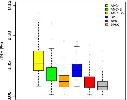
Our baseline evaluation results are shown using box and whisker plots as this helps illustrate important statistical properties. The box itself represents the range of values between quartiles (25 and 75 percentiles). The horizontal line in the middle of the box is the median. There are then vertical lines from the box to two horizontal lines, above and below it. These horizontal lines show the 5 and

7. We note that functional testing, even that requiring MCDC coverage, is not in general sufficient to determine WCETs when the hardware platform has components that cause execution times to be dependent on the execution history e.g. caches. Hence the need for an engineering margin to defineC(HI), and a non-zero probability thatC(LO)is exceeded during operation.

95 percentiles respectively. Finally there are small circles. These are the outlying values that are outside of the 5 to 95 percentile range. The box and whisker plot gives a strong indication of typical performance, the variance observed, and information about the outliers. In each figure, each scheduling scheme is coloured coded according to the legend in the top right, with the information appearing in the order AMC+, AMC+S, AMC+SG, BP, BPS, and BPSG.

Figure 3 shows the percentage of LO-criticality jobs not executed (JN E(%)) for each of the schemes, for task sets with harmonic periods. We observe that for our baseline configuration, the bailout protocol (BP) is effective in reducing the percentage of LO-criticality jobs that are not executed compared to the AMC+ scheme. Here, increasing execution time budgets (C(BU)) by making use of static slack, leads to a roughly similar reduction in

JN E(%) as BP. Since the bailout protocol and making use of static slack and gain time are complementary techniques, the BPSG scheme provides significantly better performance than AMC+SG or BP.

Figure 6 shows the results for non-harmonic task sets. Here the bailout policy is less effective at reducing the number of LO-criticality jobs not executed. This is because on average the busy periods tend to be shorter with non-harmonic task sets, with major peaks in the overall load not occurring as frequently. This means that an idle instant typically occurs shortly after entry into HI-criticality mode allowing both AMC+ and the bailout policy to recover back to LO-criticality (normal) mode in a similar time, with a similar number of LO-criticality jobs not executed.

Figures 4, 5, 7 and 8 provide further assessment of the performance of the different schemes. These results show that the percentage of time (T iH(%)) in HI-criticality mode (or bailout and recovery modes) and the number of times that the system enters HI-criticality mode as a percentage of the number of jobs of HI-criticality tasks (N iH(%)) are largest for the AMC+ scheme and smallest for BPSG. The bailout policy, which operates once HI-criticality mode is entered, does not act to reduce the number of times that the system enters HI-criticality mode, hence the

N iH(%)values are very similar for AMC+ and BP, for AMC+S and BPS, and for BPSG and AMC+SG. As expected, both statically increasing LO-criticality budgets using static slack and runtime reclamation of gain time are highly effective in reducing the number of times that the system enters HI-criticality mode (N iH(%)) and hence also the proportion of time spent in that mode (T iH(%)).

[image:11.612.332.533.64.228.2]

● ● ● ● ● ● ● ● ● ● ● ● ● ● ● ● ● ● ● ● ● ● ● ● ● ● ● ● ● ● ● ● 0.00 0.05 0.10 0.15 JNE (%) AMC+ AMC+S AMC+SG BP BPS BPSG

[image:11.612.66.269.66.227.2]

Fig. 3. Results forJ N E(%)- 80% LO-criticality Utilisation: Harmonic Periods ● ● ● ● ● ● 0.000 0.002 0.004 0.006 0.008 NiH (%) AMC+ AMC+S AMC+SG BP BPS BPSG

Fig. 4. Results forN iH(%)- 80% LO-criticality Utilisation: Harmonic Periods ● ● ● ● ● ● ● ● ● ● ● ● ● ● ● ● ● ● ● ● ● ● ● ● ● ● ● ● ● ● 0.00 0.02 0.04 0.06 0.08 0.10 TiH (%) AMC+ AMC+S AMC+SG BP BPS BPSG

[image:11.612.330.534.292.456.2]

Fig. 5. Results forT iH(%)- 80% LO-criticality Utilisation: Harmonic Periods ● ● ● ● ● ● ● ● ● ● 0.00 0.05 0.10 0.15 JNE (%) AMC+ AMC+S AMC+SG BP BPS BPSG

Fig. 6. Results forJ N E(%)- 80% LO-criticality Utilisation: Non-Harmonic Periods ● ● ● ● ● ● 0.000 0.002 0.004 0.006 0.008 NiH (%) AMC+ AMC+S AMC+SG BP BPS BPSG

Fig. 7. Results forN iH(%)- 80% LO-criticality Utilisation: Non-Harmonic Periods ● ● ● ● ● ● ● ● ● ● ● ● ● ● ● ● ● ● ● ● ● ● ● 0.00 0.02 0.04 0.06 0.08 0.10 TiH (%) AMC+ AMC+S AMC+SG BP BPS BPSG

[image:11.612.68.270.293.455.2] [image:11.612.331.533.519.681.2] [image:11.612.66.270.520.681.2]

6.4 Additional Evaluation Results: Varying Parameters

In this section, we provide additional evaluation results showing how the performance of the different scheduling schemes changes when specific parameters are varied. The parameters varied were as follows:

• LO-criticality utilisation (Default 0.8).

• _{Criticality Factor}CF _{(Ratio of HI-criticality to LO-criticality} execution time. DefaultCF = 2.0).

• Criticality ProbabilityCP (Probability that a task is of HI-criticality. DefaultCP = 0.5).

• _{Failure Probability} F P _{(Probability that a job of a} HI-criticality task exceedsC(LO). DefaultF P = 10−4_). In each of the experiments, one parameter was varied while the others were held constant at their default values. The results of these experiments show the average values of the three metrics of interest: JN E(%), N iH(%), and T iH(%). Recall that

JN E(%) is the percentage of LO-criticality jobs that are not executed,N iH(%)is the number of times HI-criticality mode is entered as a percentage of the maximum possible, i.e the total number of jobs of HI-criticality tasks. Finally,T iH(%) is the percentage of the simulation interval spent in HI-criticality mode. The experiments were repeated for both harmonic and non-harmonic task sets.

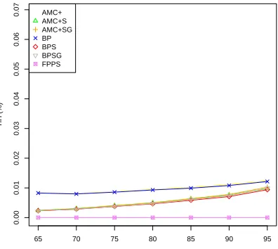
6.4.1 Varying LO-criticality utilisation

Figures 9 and 12 show how JN E(%) changes as the overall LO-criticality utilisation is varied from 0.65 to 0.95. We observe that static slack stealing for increased execution time budgets, gain time reclamation and the bailout policy are all effective in reducingJN E(%). At high utilisation levels, the basic AMC+ and BM policies result in substantially higher values ofJN E(%)

with harmonic task sets than with non-harmonic task sets. This is because with harmonic task sets conditions of peak load i.e. long processor busy periods reoccur much more frequently. Since harmonic task sets are easier to schedule8_{, using slack to increase} execution time budgets retains substantial effectiveness at high levels of utilisation (e.g. 0.95). As long processor busy periods are more frequent with harmonic task sets and become longer with increasing utilisation, in this case the bailout policy becomes more effective compared toAM C+as utilisation levels increase.

Figures 10 and 13 show howN iH(%)changes as the overall LO-criticality utilisation is varied from 0.65 to 0.95. We note that in these experiments, both static slack stealing for increased execution time budgets and gain time reclamation are effective in reducing the number of times HI-criticality mode is entered. As expected; however, the bailout policy has no noticeable effect compared to AMC+. This is because the bailout policy only comes into effect once HI-criticality mode has been entered.

Figures 11 and 14 show howT iH(%)changes as the overall LO-criticality utilisation is varied from 0.65 to 0.95. Here there are clear differences in performance between harmonic and non-harmonic task sets. With non-non-harmonic task sets, there are very few long busy periods thus when HI-criticality mode is entered it is soon exited as an idle instant is reached. This means that the percentage of the total time spent in the HI-criticality mode is much less than with harmonic tasks sets, and also explain why the bailout policy is unable to significantly reduce the time in HI-criticality mode. This is also the case with gain time reclamation,

8. The utilisation bound is 1 for pure harmonic task sets and 0.69 for non-harmonic task sets.

since the busy periods are too short for substantial gain time to accumulate and prevent the transition to HI-criticality mode. Static slack stealing for increased execution time budgets is still effective in this case, since it reduces the number of times HI-criticality mode is entered which impacts the total time in that mode.

6.4.2 Varying the Criticality Factor (CF)

Figures 15 and 18 show howJN E(%)changes as the Criticality Factor (CF) is varied from 1.25 to 2.5.

We observe that with harmonic task sets,JN E(%)decreases with increasing CF for the BM and AMC+ schemes. This is because with small values ofCF, schedulable task sets can be generated that include low priority but HI-criticality tasks with long periods and long execution times. The presence of such tasks increases the time in HI-criticality mode (see Figure 17) and thus alsoJN E(%). This effect is not apparent with non-harmonic task sets since they are much harder to schedule and so do not readily permit such tasks.

In both the harmonic and non-harmonic cases, the use of both static slack stealing to increase execution time budgets and gain time reclaiming are highly effective in reducing the number of times that the system enters HI-criticality mode (N iH(%)), thus also reducing the amount of time spent in that mode (T iH(%)) -see Figures 16 to 20. These techniques have less effect as the value ofCF increases, since they have to mitigate the increasing effect of longer HI-criticality execution times.

6.4.3 Varying the Criticality Probability (CP)

Figures 21 to 26 show howJN E(%),N iH(%), andT iH(%)

change as the Criticality Probability (CP) controlling the proportion of HI-criticality tasks varies from 0.3 to 0.7. Here the key behaviours of the schemes remain as reported for the baseline configurations discussed in detail in section 6.3. The predominant effect of increasing the proportion of HI-criticality tasks is to increase the number of times that the system enters HI-criticality mode and thus also the proportion of LO-criticality jobs not executed and the proportion of time spent in HI-criticality mode. TheN iH(%)value remains relatively constant since that measure is normalised to the number of HI-criticality jobs.

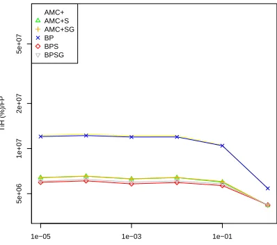
6.4.4 Varying the Failure Probability (F P)

Figures 27 to 32 show how the normalized metrics

JN E(%)/F P, N iH(%)/F P, and T iH(%)/F P change as the Failure Probability (F P) controlling the proportion of HI-criticality jobs that exceed their LO-criticality execution time budget varies from10−5_{to1. These graphs show that the metrics}

JN E(%),N iH(%), andT iH(%)have an approximately linear relationship with the Failure Probability for Failure Probabilities of

10−2_{and below, taking nearly constant values for each scheduling} scheme. The figures show that the relative performance of the various schemes is effectively independent of the likelihood of HI-criticality tasks exhibiting HI-criticality behavior. At very high Failure Probabilities e.g. 10−1 _{= 0.1 and 1, then there are} typically multiple jobs exhibiting HI-criticality behavior within each HI-criticality mode interval. Thus the metricJN E(%)/F P

65 70 75 80 85 90 95

0.00

0.02

0.04

0.06

0.08

0.10

UTIL

JNE (%)

●

● ● ●

● ●

● ●AMC+

[image:13.612.334.532.64.246.2]

AMC+S AMC+SG BP BPS BPSG FPPS

Fig. 9. J N E(%) Results varying LO-criticality Utilisation: Harmonic Periods

65 70 75 80 85 90 95

0.000

0.002

0.004

0.006

0.008

0.010

UTIL

NiH (%)

● ● ● ● ● ● ● ●AMC+

[image:13.612.68.270.65.246.2]

AMC+S AMC+SG BP BPS BPSG FPPS

Fig. 10.N iH(%)Results varying LO-criticality Utilisation: Harmonic Periods

65 70 75 80 85 90 95

0.00

0.01

0.02

0.03

0.04

0.05

0.06

0.07

UTIL

TiH (%) ●

● ● ●

● ●

● ●AMC+

AMC+S AMC+SG BP BPS BPSG FPPS

Fig. 11.T iH(%)Results for varying LO-criticality Utilisation: Harmonic Periods

65 70 75 80 85 90 95

0.00

0.02

0.04

0.06

0.08

0.10

UTIL

JNE (%) ● ● ● ●

● ●

● ●AMC+

[image:13.612.68.271.292.473.2]

AMC+S AMC+SG BP BPS BPSG FPPS

Fig. 12.J N E(%)Results varying LO-criticality Utilisation: Non-Harmonic Periods

65 70 75 80 85 90 95

0.000

0.002

0.004

0.006

0.008

0.010

UTIL

NiH (%)

● ● ● ● ● ● ● ●AMC+

AMC+S AMC+SG BP BPS BPSG FPPS

Fig. 13.N iH(%)Results varying LO-criticality Utilisation: Non-Harmonic Periods

65 70 75 80 85 90 95

0.00

0.01

0.02

0.03

0.04

0.05

0.06

0.07

UTIL

TiH (%)

● ● ● ● ● ● ● ●AMC+

AMC+S AMC+SG BP BPS BPSG FPPS

[image:13.612.334.531.292.472.2] [image:13.612.334.532.520.697.2] [image:13.612.69.269.521.699.2]

1.0 1.5 2.0 2.5

0.00

0.02

0.04

0.06

0.08

0.10

CF

JNE (%)

●

●

● ●

● ● ●AMC+

AMC+S AMC+SG BP BPS BPSG FPPS

Fig. 15.J N E(%)Results varying the Criticality Factor (CF): Harmonic Periods

1.0 1.5 2.0 2.5

0.000

0.002

0.004

0.006

0.008

0.010

CF

NiH (%)

● ● ● ● ● ● ●AMC+

[image:14.612.334.531.66.243.2]

AMC+S AMC+SG BP BPS BPSG FPPS

Fig. 16.N iH(%)Results varying the Criticality Factor (CF): Harmonic Periods

1.0 1.5 2.0 2.5

0.00

0.02

0.04

0.06

0.08

CF

TiH (%)

●

●

● ●

● ● ●AMC+

[image:14.612.68.270.67.244.2]

AMC+S AMC+SG BP BPS BPSG FPPS

Fig. 17.T iH(%)Results for varying the Criticality Factor (CF): Harmonic Periods

1.0 1.5 2.0 2.5

0.00

0.02

0.04

0.06

0.08

0.10

CF

JNE (%) ● ● ●

● ●

● ●AMC+

[image:14.612.334.531.293.468.2]

AMC+S AMC+SG BP BPS BPSG FPPS

Fig. 18. J N E(%) Results varying the Criticality Factor (CF): Non-Harmonic Periods

1.0 1.5 2.0 2.5

0.000

0.002

0.004

0.006

0.008

0.010

CF

NiH (%)

● ● ● ● ● ● ●AMC+

[image:14.612.68.272.293.469.2]

AMC+S AMC+SG BP BPS BPSG FPPS

Fig. 19. N iH(%) Results varying the Criticality Factor (CF): Non-Harmonic Periods

1.0 1.5 2.0 2.5

0.00

0.02

0.04

0.06

0.08

CF

TiH (%)

● ● ● ● ● ● ●AMC+

AMC+S AMC+SG BP BPS BPSG FPPS

[image:14.612.333.532.520.695.2]

0.3 0.4 0.5 0.6 0.7

0.00

0.02

0.04

0.06

0.08

0.10

CP

JNE (%)

●

●

●

●

● ●AMC+

[image:15.612.70.269.65.244.2]

AMC+S AMC+SG BP BPS BPSG FPPS

Fig. 21. J N E(%) Results varying the Criticality Probability (CP): Harmonic Periods

0.3 0.4 0.5 0.6 0.7

0.000

0.002

0.004

0.006

0.008

0.010

CP

NiH (%)

● ● ● ● ●

[image:15.612.335.532.66.245.2]

●AMC+ AMC+S AMC+SG BP BPS BPSG FPPS

Fig. 22. N iH(%) Results varying the Criticality Probability (CP): Harmonic Periods

0.3 0.4 0.5 0.6 0.7

0.00

0.01

0.02

0.03

0.04

0.05

0.06

CP

TiH (%)

●

●

●

●

● ●AMC+

AMC+S AMC+SG BP BPS BPSG FPPS

Fig. 23.T iH(%) Results for varying the Criticality Probability (CP): Harmonic Periods

0.3 0.4 0.5 0.6 0.7

0.00

0.02

0.04

0.06

0.08

0.10

CP

JNE (%)

●

●

●

●

● ●AMC+

[image:15.612.336.532.293.472.2]

AMC+S AMC+SG BP BPS BPSG FPPS

Fig. 24.J N E(%)Results varying the Criticality Probability (CP): Non-Harmonic Periods

0.3 0.4 0.5 0.6 0.7

0.000

0.002

0.004

0.006

0.008

0.010

CP

NiH (%)

● ● ● ● ●

●AMC+ AMC+S AMC+SG BP BPS BPSG FPPS

Fig. 25.N iH(%)Results varying the Criticality Probability (CP): Non-Harmonic Periods

0.3 0.4 0.5 0.6 0.7

0.00

0.01

0.02

0.03

0.04

0.05

0.06

CP

TiH (%)

●

●

●

●

● ●AMC+

AMC+S AMC+SG BP BPS BPSG FPPS

[image:15.612.334.531.520.698.2] [image:15.612.69.275.522.700.2]

1e−05 1e−03 1e−01

100

200

500

1000

2000

FP

JNE (%)/FP

● ● ● ● ● ● ●AMC+

[image:16.612.334.531.66.243.2]

AMC+S AMC+SG BP BPS BPSG

Fig. 27.J N E(%)Results varying the Failure Probability (F P): Harmonic Periods

1e−05 1e−03 1e−01

20

50

100

200

FP

NiH (%)/FP

● ● ● ● ● ● ●AMC+

[image:16.612.69.267.67.244.2]

AMC+S AMC+SG BP BPS BPSG

Fig. 28.N iH(%)Results varying the Failure Probability (F P): Harmonic Periods

1e−05 1e−03 1e−01

5e+06

1e+07

2e+07

5e+07

FP

TiH (%)/FP

● ● ● ● ● ● ●AMC+

AMC+S AMC+SG BP BPS BPSG

Fig. 29. T iH(%) Results for varying the Failure Probability (F P): Harmonic Periods

1e−05 1e−03 1e−01

100

200

500

1000

2000

FP

JNE (%)/FP

● ● ● ● ● ● ●AMC+

[image:16.612.67.268.292.471.2]

AMC+S AMC+SG BP BPS BPSG

Fig. 30.J N E(%)Results varying the Failure Probability (F P): Non-Harmonic Periods

1e−05 1e−03 1e−01

20

50

100

200

FP

NiH (%)/FP

● ● ● ● ● ● ●AMC+

[image:16.612.332.531.293.471.2]

AMC+S AMC+SG BP BPS BPSG

Fig. 31.N iH(%)Results varying the Failure Probability (F P): Non-Harmonic Periods

1e−05 1e−03 1e−01

5e+06

1e+07

2e+07

5e+07

FP

TiH (%)/FP

● ● ● ● ● ● ●AMC+

AMC+S AMC+SG BP BPS BPSG

[image:16.612.332.531.520.696.2] [image:16.612.69.269.521.696.2]