GreenTouch GreenMeter Core Network Energy-Efficiency Improvement Measures and Optimization

This is a repository copy of

GreenTouch GreenMeter Core Network Energy-Efficiency

Improvement Measures and Optimization

.

White Rose Research Online URL for this paper:

http://eprints.whiterose.ac.uk/126860/

Version: Accepted Version

Article:

Elmirghani, JMH, Klein, T, Hinton, K et al. (5 more authors) (2018) GreenTouch

GreenMeter Core Network Energy-Efficiency Improvement Measures and Optimization.

IEEE/OSA Journal of Optical Communications and Networking, 10 (2). A250-A269. ISSN

1943-0620

https://doi.org/10.1364/JOCN.10.00A250

© 2018 Optical Society of America/IEEE Personal use of this material is permitted.

Permission from IEEE must be obtained for all other users, including reprinting/

republishing this material for advertising or promotional purposes, creating new collective

works for resale or redistribution to servers or lists, or reuse of any copyrighted

components of this work in other works.

[email protected] https://eprints.whiterose.ac.uk/ Reuse

Unless indicated otherwise, fulltext items are protected by copyright with all rights reserved. The copyright exception in section 29 of the Copyright, Designs and Patents Act 1988 allows the making of a single copy solely for the purpose of non-commercial research or private study within the limits of fair dealing. The publisher or other rights-holder may allow further reproduction and re-use of this version - refer to the White Rose Research Online record for this item. Where records identify the publisher as the copyright holder, users can verify any specific terms of use on the publisher’s website.

Takedown

If you consider content in White Rose Research Online to be in breach of UK law, please notify us by

GreenTouch GreenMeter Core Network Energy

Efficiency Improvement Measures and

Optimization [Invited]

J.M.H. Elmirghani

_{, T. Klein}

_{, K. Hinton}

_{, L. Nonde}

_{, A. Q. Lawey}

_{, T.E.H. El-Gorashi}

_{, M.O.I. Musa}

_,

X. Dong

School of Electronic and Electrical Engineering, University of Leeds, LS2 9JT, UK

_,

Bell Labs, Nokia, Murray Hill, NJ, USA

_,

Centre for Energy-Efficient Telecommunications, University of Melbourne, Australia

_,

Qualcomm Technologies International, UK

_,

Huawei Shannon Lab, Huawei Technologies, Shenzhen, China

Abstract—

improvements in core networks obtained as a result of work carried out by the GreenTouch consortium over a 5 year period. A number of techniques that yield substantial energy savings in core networks were introduced including: (i) the use of improved network components with lower power consumption, (ii) putting idle components into sleep mode, (iii) optically bypassing intermediate routers, (iv) the use of mixed line rates (MLR), (v) placing resources for protection into a low power state when idle, (vi) optimization of the network physical topology, (vii) the optimization of distributed clouds for content distribution and network equipment virtualization. These techniques are recommended as the main energy efficiency improvement measures for 2020 core networks. A mixed integer linear programming (MILP) optimization model combining all the aforementioned techniques was built to minimize energy consumption in the core network. We consider group 1 nations traffic and place this traffic on a US continental network represented by the AT&T network topology. The projections of the 2020 equipment power consumption are based on two scenarios: a business as usual (BAU) scenario and a GreenTouch (GT) (i.e. BAU+GT) scenario. The results show that the 2020 BAU scenario improves the network energy efficiency by a factor of 4.23x compared to the 2010 network as a result of the reduction in the network equipment power consumption. Considering the 2020 BAU+GT network, the network equipment improvements alone reduce network power by a factor of 20x compared to the 2010 network. Including of all the BAU+GT energy efficiency techniques yields a total energy efficiency improvement of 315x. cWe have also implemented an experimental demonstration that illustrates the feasibility of energy efficient content distribution in IP/WDM networks.

Keywords—Cloud Networks; Virtual Network Embedding; Network Virtualization; MILP; Energy Efficient Networks; IP over WDM.

I.

INTRODUCTION

Internet traffic has been growing exponentially as a result of the continuously growing popularity of data intensive applications and the increasing number of devices connected to the Internet. It is estimated that by 2020 there will be over 50 billion devices connected to the Internet [1]. The Internet service model as we know it today is evolving to facilitate

efficient communication and service provisioning. Cloud computing is at the centre of this evolution. One of the main challenges facing cloud computing is serving the increasing traffic demand adequately while maintaining sustainability and enhancing the profit margins through lower energy usage. Today the power consumption of networks is a significant contributor to the total power demand in many developed countries. For example, in the winter of 2007, British Telecom became the largest single power consumer in the UK

accounting for 0.7% of the total UK’s power consumption [2].

Driven by the economic, environmental and societal impact, significant academic and industrial research effort has been focused recently on reducing the power consumption of communication networks.

GreenTouch was a consortium of leading Information and Communications Technology (ICT) research experts. It includes approximately 50 academic, industry and non-governmental organizations and played an essential role in technology breakthroughs in communication network energy efficiency. The consortium was formed in 2010 to pursue the ambitious goal of bridging the gap between traffic growth and network energy efficiency. This is to be achieved by delivering architecture specifications and technologies needed to increase energy efficiency by a factor of 1000 compared to 2010 levels. Achieving this goal will help create a sustainable future for data networking and the Internet. The research areas investigated by GreenTouch included; wired access networks, mobile networks, core networks and services, policies and standards. Wireless networks are expected to achieve the highest savings followed by access networks and finally core networks.

Programming (MILP) model that jointly optimizes the design of content distribution services [11], virtual machines (VMs) placement [11], virtual network embedding (VNE) [12] in IP over WDM networks for energy efficiency, (ii) introducing an energy efficient protection scheme where protection resources are switched off when idle, (iii) developing new models for equipment power consumption, (iv) considering revised 2020 traffic strands, (v) evaluating the energy efficient model over a new continental US topology using the city locations of the AT&T network.

The total power consumption is evaluated considering a 2010 network and a 2020 network. For the 2010 network we consider the traffic in 2010 along with the most energy-efficient commercially available equipment at that time. The 2020 network is based on projections of the traffic in 2020 and the reductions in the equipment power consumption by 2020. The projections of the 2020 equipment power consumption are based on two scenarios: a business as usual (BAU) scenario and BAU+GT scenario where the technical advances achieved by the GreenTouch consortium will accelerate the reduction in equipment power consumption.

The base year of 2010 was taken because that was the year GreenTouch commenced operation and it was a year for which a reasonable amount of data on traffic and technology evolution was available. The traffic trend changes between 2010 and 2015 are included in the model. In particular, the growing dominance of video traffic and the evolution toward Content Delivery Networks (centralized and decentralized) are included. In terms of technology trends, it should be noted that the focus of the GreenMeter (and GreenTouch in general) was on the energy

savings available if the network is based

on optimizing technology for energy efficiency; not on actual commercial equipment evolution or the impact of the economic cycle over those years. The Business As Usual technology forecasts were based upon the evolution up to 2015. These trends are still relevant to 2020.

Network operators have traditionally and currently focused on network cost. In fact, until recently, most operators focused almost solely on CAPEX and it is only over the last decade that Total Cost of Ownership (TCO = CAPEX + OPEX) has started to be considered. As operators have started to consider OPEX, many have realized that OPEX can actually dominate CAPEX over a sufficiently long duration. Energy consumption is becoming an increasingly important component of OPEX. However, although important, this is not the main raison d'etre for this work. The point which this paper makes is that an increased focus on network sustainability (i.e. energy efficiency) can provide dramatic reductions in energy consumption. Energy efficiency, as with many aspects of large scale construction, is best "built in" as compared to "retro-fitted". The purpose of the GreenMeter paper is to provide a road-map for network operators to build-in energy efficiency as well as showing them the potential energy savings that can be attained. Although a focus on CAPEX (and more recently OPEX) has been traditional to date, it is well accepted that in the future an increasing number of organizations will move toward "triple bottom line" style accounting. This means modelling, such as provided by the GreenMeter, will be of interest as this trend continues.

The reminder of this paper is organized as follows: In Section II, we present the cloud computing services over core networks considered for the energy efficiency improvement. In Section III, we provide the detailed MILP formulation and introduce the methods used to determine the network equipment power consumption improvements and the calculations of router port power consumption in Section IV. The network traffic for 2010 and 2020 networks used in the model is presented in Section V.

The results of the MILP model are discussed and analyzed in Section VI. We present an experimental demonstration of energy efficient content distribution in Section VII. The paper is finally concluded in Section VIII.

II. ENERGY EFFICIENT CLOUD COMPUTING

SERVICES OVER CORE NETWORKS Cloud computing has now grown into a widely accepted computing paradigm and its significance is expected to grow even more in the coming years. Virtualization lies at the heart of cloud computing where the requested services are provisioned, removed and managed over existing physical infrastructure such as servers, storage and networks. Our work in [12] investigates the energy efficiency benefits of virtualization and our work in [11] investigates energy efficient design of cloud computing services in core networks that address the optimal way of distributing content and the replication of VMs. In this work, we have combined virtualization, replication and content distribution for a 2020 network with BAU+GT equipment as well as all the aforementioned techniques of bypass, sleep, MLR and topology optimization.

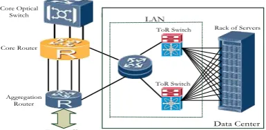
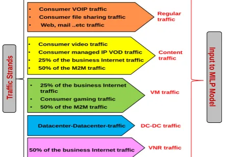
We considered the total 2020 traffic [14], [15], [16] according to the traffic strands shown in Fig. 2. As shown in Fig. 1, a typical cloud data center consists of three main parts, namely; servers, internal LAN and storage. We are not focusing on the energy efficiency inside data centers, a subject that has been extensively researched by the Green Grid consortium [13] and others. Cloud data centers are usually co-located with core network nodes to benefit from the large bandwidth offered by such nodes.

1. Cloud Content Delivery and Virtual Machine Slicing In cloud content delivery, we serve requests from clients by selecting the optimal number of clouds and their locations in the network so that the total power is minimized. A decision is also made on how to replicate content according to content popularity so that minimum power is consumed when delivering content. Machine virtualization provides an economical solution that enables efficient utilization of physical resources in clouds. Our model optimizes the placement of VMs to minimize energy consumption. In this case, a VM is a logical entity created in response to a service request by one or more users sharing that particular VM. The VM therefore consumes power due to both processing requirements and due to the traffic generated between the VM and the user. We optimize the placement of VMs within the clouds as demand varies during the day to minimize the network power consumption. The VM placement scheme under consideration is referred to as VM Slicing. Under this scheme, incoming requests are distributed among different copies of the same VM to serve a smaller number of users. Each copy of the VM, ie a slice, has less CPU requirements compared to the original VM. VM slicing is the most energy efficient approach compared to other VM placement schemes as we have discussed in [11] because slicing does not increase the data center cloud power consumption allowing the VM slices to be distributed over the network.

Fig. 1: Cloud Data Center Architecture LAN

ToR Switch

ToR Switch

Rack of Servers

Data Center Core Router

Aggregation Router Core Optical

Switch

Fig. 2: Traffic Strands for Distributed Cloud for Content Delivery and Network Virtualization

2. Network Virtualization

The success of future cloud networks will greatly depend on network virtualization [17]. Here clients are expected to be able to specify both bandwidth and processing requirements for hosted applications and services. The network virtualization ability to allow multiple heterogeneous virtual networks (VNs) to coexist on one physical platform consolidates resources, which in turn leads to potential energy savings. The network is broken down into multiple VN slices which are requested by enterprise clients and provisioned by infrastructure providers (InPs). A VN is a logical topology made up of a set of virtual nodes (which can be routers, switches, VMs, etc) interconnected by virtual links. Enterprise clients send virtual network requests (VNRs) to a cloud infrastructure provider in order to obtain a slice of the network that meets their specific requirements. Our model determines the optimal way of embedding VNRs in the core network with clouds so that the power consumption in the network is minimized.

III.

MILP Model

In this section we introduce the Mixed Integer Linear Programming (MILP) model that combines the cloud content delivery model [11], the virtual machine placement model [11] and the virtual network embedding model [12] to collectively design energy-efficient cloud service provisioning in an IP over WDM network. The IP over WDM network incorporates all the techniques that were considered in [4] including optical bypass, mixed line rates (MLR), energy efficient routing, sleep and physical topology optimization.

Given the client requests for content and VMs and the VNRs, the model responds by selecting the optimal number of clouds and their locations in the network as well as the capability of each cloud so that the network and data center clouds power consumption is minimized. The model decides how to replicate content in the cloud according to its popularity so the minimum power possible is consumed in delivering content. We have assumed that the popularity of the different objects of the content follows a Zipf distribution. Content has been divided into equally sized popularity groups. A popularity group contains objects of similar popularity. The number and locations of content replicas are optimized based on content popularity. The model also optimizes the placement of VMs as demands vary throughout the day to minimize the total power consumption. In virtual network provisioning, the model efficiently embeds virtual nodes and embeds the bandwidth demands of links associated with VNRs in cloud data centers and in the network respectively to minimize the total power consumption.

In the 2020 BAU+GT network, intelligent management of protection resources is introduced where resources are activated

only when required reducing the network power consumption to about the half. Note that protection uses 1+1 protection where a protection resource is used for each active resource. We first introduce the parameters and variables related to the different cloud services and the IP over WDM network.

Parameters:

Cloud Content Delivery

Set of popularity groups

Cloud power usage effectiveness (unitless)

Storage power consumption (Watts)

Storage capacity of one storage rack (GByte)

Storage and switching redundancy (unitless) Storage power consumption per GB,

(Watts/GByte)

Storage utilization (unitless)

Popularity group storage size, G (GByte)

Content server capacity (Gbit/sec)

Content server energy per bit (Joule/bit)

Cloud switch power consumption (Watts)

Cloud switch capacity (Gbit/sec)

Cloud switch energy per bit, (Joule/bit)

Cloud router power consumption (Watts)

Cloud router capacity (Gbit/sec)

Cloud router energy per bit, (Joules/bit) Popularity of object (Zipf distribution, unitless) Traffic from distributed datacenters to node d (Gbit/sec) Fraction of that is generated by content (unitless) Traffic from distributed datacenters to node d generated by content,

(Gbit/sec)

Traffic from Popularity group to node d (Gbit/sec)

Content synchronization traffic from the central cloud data center to any other cloud data center (Gbit/sec)

Data centre to data centre traffic due to content delivery between the central cloud and the remote cloud (Gbit/sec)

Cloud Virtual Machines Set of VMs

Power consumption per single core of a VM (Watts) Total number of VMs

Number of cores for VM v

Fraction of traffic due to VMs (unitless) Traffic from distributed clouds to node d due to virtual machines, (Gbit/sec)

Traffic from virtual machine v to node d, (Gbit/sec)

Virtual machine synchronization traffic between any cloud pair when there are cloud data centers in the network (Gbit/sec) Total DC-DC traffic in the network with clouds (Gbit/sec) Data centre to data centre traffic due to virtual machines between a cloud data center at and the remote cloud data center (Gbit/sec)

; Total DC to DC traffic due to content and virtual machines (Gbit/sec)

Virtual Network Embedding

Set of virtual network requests

RV Set of nodes in a virtual network request Total number of data centers in the network

if the master node of VNR is located at substrate node , otherwise

BR Bandwidth requested by VNR on virtual link , ) (Gbit/sec) The number of virtual cores requested by virtual machine of

VNR

• Consumer VOIP traffic

• Consumer file sharing traffic

• Web, mail ..etc traffic

• Consumer video traffic

• Consumer managed IP VOD traffic

• 25% of the business Internet traffic

• 50% of the M2M traffic

Datacenter-Datacenter-traffic

50% of the business Internet traffic

Traffic Stran

d

s

In

pu

t to

MIL

P

Mod

el

• 25% of the business Internet traffic

• Consumer gaming traffic

• 50% of the M2M traffic

Regular traffic

Content traffic

VM traffic

DC-DC traffic

IP/WDM

Set of IP/WDM nodes Set of neighbors of node i Set of wavelength rates

Router port power consumption at line rate (Watts) Transponder power consumption at line rate (Watts) EDFA power consumption (Watts)

Power consumption of optical switch at node (Watts) Multi/demultiplexer power consumption (Watts)

Regenerator power consumption at line rate (Watts) Number of wavelengths per fiber

Wavelength rate at line rate r (Gbit/sec) Max span distance between EDFAs (km) Distance between node pair (m,n) (km) Number of EDFAs between node pair (m,n) IP/WDM network power usage effectiveness (unitless) A large enough number

Number of regenerators at line rate between node pair (m,n) Number of physical links for the optimized topology minimum nodal degree for the optimized topology (unitless)

Regular traffic between node pair (s,d) (Gbit/sec)

Variables

Cloud Content Delivery

if popularity group p is placed in node s to serve users

in node d, otherwise

Traffic generated due to placing popularity group p in node s to serve users in node d (Gbit/sec)

Content delivery traffic from cloud s to users in node d (Gbit/sec) Cloud s upload capacity for content delivery (Gbit/sec)

if cloud s stores a copy of popularity group p, otherwise

if a cloud is built in node s to deliver content, otherwise

Number of content servers in cloud s Number of clouds in the network

Number of switches in cloud s for content delivery Number of routers in cloud s for content delivery Cloud s storage capacity (GBytes)

Cloud VM

Traffic demand from VM v in cloud s to node d (Gbit/sec) Total traffic to users due to VMs (Gbit/sec)

=1 if cloud s hosts a copy of VM v, otherwise Total number of cores in Cloud s

Number of processing servers in cloud s

Cloud s upload rate capacity for virtual machines (Gbit/sec) if a cloud is built in node s to host

virtual machines, otherwise. Number of clouds hosting virtual machines

if , , otherwise.

A binary indicator that is 1 if there is a cloud data center at and another cloud data center at for the case when the number of total clouds are in the network

An integer taking values

Virtual Network Embedding

if substrate node is a data center, otherwise

= 1, if the embedding of virtual nodes and of virtual request in substrate nodes and ,

respectively is successful and a link is established if a virtual link of VNR exists.

FE _{FE , if all the links of VNR are fully embedded in the}

substrate network, otherwise FE

= 1, if node of VNR is embedded in substrate node ,

otherwise = 0.

is the XOR of and , i.e.

FN FN , if all the nodes of a VNR are fully embedded in the substrate network, otherwise FN

Total traffic demand on IP link due to the embedded links of all VNRs (Gbit/sec)

if virtual machine of VNR has been embedded at the cloud at node otherwise

is the XOR of and , i.e. ,

if either or is equal to 1, otherwise .

Virtual nodes consolidation factor which defines the maximum number of virtual nodes of a VNR that can be co-located at a substrate node

IP/WDM

Number of wavelengths of rate in the virtual link (i,j) Total traffic in the network between node pair (s,d) (Gbit/sec) Traffic flow between node pair (s,d) traversing virtual link (i,j) (Gbit/sec)

Number of wavelengths of rate in the virtual link (i,j) traversing physical link (m,n)

Total number of used wavelengths of rate in the physical link (m,n)

Total number of fibers on the physical link (m,n)

if a physical link (m,n) is present otherwise, Number of aggregation ports at rate

Number of protection wavelengths of rate in the virtual link (i,j) traversing physical link (m,n).

if , otherwise

if , otherwise

Under the bypass approach, the total IP over WDM network

power consumption ( ) is composed of:

1. The power consumption of router ports

2. The power consumption of transponders

3. The power consumption of EDFAs

4. The power consumption of regenerators

5. The power consumption of optical switches

1. The power consumption of content servers

2. The power consumption of switches and routers in data centers due to content

3. The power consumption due to storage

4. The power consumption due to virtual machines

5. The power consumption of switches and routers in DC due to virtual machines

Objective:

Minimize

(1)

Subject to:

Content delivery cloud constraints

IP/WDM network traffic due to content placement:

(2)

(3)

(4)

(5)

Constraint (2) calculates the traffic generated in the IP/WDM network due to requesting popularity group p that is placed in node s by users located in node d. Constraint (3) ensures that each popularity group request is served from a single cloud only. We have not included traffic bifurcation where a user may get parts of the content from different clouds. Constraint (4) calculates the traffic from the content cloud in node s and users in node d. Constraint (5) calculates the content upload rate of each cloud based on content traffic sent from the cloud.

Popularity groups locations:

(6)

(7)

Constraints (6) and (7) ensure that popularity group p is replicated to cloud s if cloud s is serving requests for this

popularity group, where M is a large enough unitless number to

ensure that when .

Cloud location and number of clouds:

(8)

(9)

(10)

Constraints (8) and (9) build a cloud in location s if that location is chosen to store at least one popularity group or more, where

M is a large enough unitless number to ensure that

when is greater than zero. Constraint (10) calculates

total number of content clouds in the network.

Cloud Capability:

(11) (12) (13) (14)

Constraints (11)-(13) calculate the number of content servers, switches and routers required at each cloud based on content upload traffic going through these elements. Note that the

number of switches is calculated considering

redundancy. Constraint (14) calculates the storage capacity needed in each cloud based on the number of replicated popularity groups.

VM Replication constraints

VMs demand:

(15)

Constraint (15) ensures that the requests of users in all nodes are satisfied by the VMs placed in the network.

Virtual Machines locations:

(16)

(17)

Constraints (16) and (17) replicate VM v to cloud s if cloud s is selected to serve requests for v where M is a large enough

number, with units of Gbps, to ensure that when

.

Clouds locations:

(18)

(19)

Constraints (18) and (19) build a cloud in location s if the location is selected to host one or more VMs where M is a large

enough unitless number to ensure that when

.

(20)

Constraint (20) calculates the number of VM cores in each cloud s due to VM placement

Inter Cloud Traffic for Content

(21)

Constraint (21) calculates the data center to data center traffic between the central cloud and the remote cloud . We assume that the central cloud is located at node 11 in the network because of its location and high nodal degree.

Inter Cloud Traffic for VMs due to placement

(22)

(23)

(24)

Constraints (22), (23) and (24) convert the number of virtual machine data center clouds ( ) into an index for the

binary variable . Therefore if ,

, otherwise.

(25)

Constraint (25) ensures that 1 if there is a cloud data center at and another cloud data center at for the case when the total number of cloud data centers is in the network,

0, otherwise.

(26)

Constraint (26) calculates the data center to data center traffic due to virtual machines.

Virtual Network Embedding

Node Embedding Constraints

(27)

(28)

(29)

(30)

(31)

Constraint (27) ensures that the requested virtual cores do not exceed the capacity of the data centre. Constraint (28) ensures that virtual machines are embedded in nodes with data centers

by implementing the AND operation of and

. Constraint (29) ensures that each virtual machine is only embedded once in the network. Constraint (30) gives the number of data centers. Constraint (31) gives the number of virtual nodes from the same request that can be co-located in the same data centre.

(32)

Constraint (32) ensures that each virtual node is only embedded once in the network.

FN (33)

Constraint (33) ensures that virtual machines of a VNR are completely embedded meeting all their CPU demands

Link Embedding Constraints

(34)

Constraint (34) ensures that virtual nodes connected in the VNR are also connected in the substrate network. We achieve this by introducing a binary variable which is only equal to 1 if and are exclusively equal to 1 otherwise it is zero.

(35)

Constraint (35) ensures that the bidirectional traffic flows are maintained after embedding the virtual links.

BR (36)

Constraint (36) generates the traffic demand matrix resulting from embedding the VNRs in the substrate network.

BR FE _{BR (37)}

Constraint (37) ensures that the bandwidth demands of a VNR are completely embedded.

FE _{FN (38)}

Constraint (38) ensures that both nodes and links of a VNR are embedded.

IP/WDM Network Constrains

Total Traffic constraint

Constraint (39) calculates the total traffic to be routed in the IP over WDM network resulting from Content delivery, VMs placement, the embedding of virtual network requests, datacenter to datacenter traffic and regular traffic.

Flow conservation constraint in the IP layer:

(40)

Constraint (40) represents the flow conservation constraint in the IP layer. It ensures that in all nodes the total outgoing traffic is equal to the total incoming traffic except for the source and the destination nodes. It also ensures that traffic flows can be split and transmitted through multiple flow paths in the IP layer. Virtual IP link capacity constraint: (41)

Constraint (41) ensures that the summation of all traffic flows through a virtual link does not exceed its capacity. Flow conservation constraint in the optical layer: W (42)

Constraint (42) represents the flow conservation constraint in the optical layer. It represents the fact that in all nodes the total outgoing wavelengths of a virtual link should be equal to the total incoming wavelengths except for the source and the destination nodes of the virtual link. Number of aggregation ports: (43)

Constraint (43) calculates the number of router aggregation points at any given line rate for each node in the network. Flow conservation and virtual link capacity constraints for protection lightpaths: (44)

Constraint (44) represent the flow conservation constraint in the optical layer for the protection links. Link disjoint Protection: 45)

(46)

(47)

(48)

+ (49)

i W i j m n Constraints (45)-(49) link the non-binary variables and with their binary counterparts and respectively. Constraint (49) ensures that a working path and its protection path are link disjoint. Physical topology design: Physical link capacity constraints: (50)

W (51)

Constraints (50) and (51) are the physical link capacity constraints. Constraint (50) ensures that the total number of wavelength channels in working and protection virtual links traversing a physical link does not exceed the maximum capacity of fibers in the physical link. Constraint (51) ensures that the number of wavelength channels in working and protection virtual links traversing a physical link is equal to the number of wavelengths in that physical link. Physical links binary variables: (52) (53) Constraints (52) and (53) are used to link the non-binary variable with its binary counterpart to indicate if a phyiscal link between two nodes is present or not. Bidirectional Links: (54) Constraint (54) ensures that any connected pair of nodes is connected in both directions.

Number of links constraint:

Constraint (55) ensures that the total number of links in the network does not exceed the limit on the number of links. This allows network designers to select a maximum number of links to be deployed and request that the traffic is served under this constraint. This constraint can be removed to allow the MILP to select the optimal number of links to be deployed.

Nodal degree limit constraint:

Constraint (56) gives the minimum nodal degree. Note that a limit on the minimum nodal degree is needed to ensure connectivity i.e. the node is not isolated from the network (even after a number of link failures).

IV. EQUIPMENT POWER CONSUMPTION

The reference point for power consumption improvements is the 2010 network. In the 2010 network, the best commercially deployed equipment in terms of both power consumption and capacity is used. We considered the power consumption of the following network elements in the IP/WDM network; (i) Routers (ii) Transponders (iii) Regenerators (iv) Erbium Doped Fiber Amplifiers (EDFAs) and (v) Optical Switches. The router port power consumption for 2010 is quoted at 40Gbps and it includes the share of the aggregate power (switching fabric, router processor, power module and other power consuming elements including fans and their controllers) apportioned to the 40Gbps port. The power consumption of transponders and regenerators is also quoted at 40Gbps line rate and accounts for both the optical and electronic subsystems of the equipment.

1.

Calculation of Router Port Power Consumption

The router port power consumption calculations are based on the Cisco CRS-1 16-Slot Chassis [18] and the Cisco CRS-X 16-Slot Chassis [19]. Two methods of calculating the router port power consumption of a given line rate were considered. In

method 1, a linear approximation method was used to determine the energy per bit , , in W/Gbps. In this method, the total

chassis power consumption , given in the Cisco CRS-1

datasheet, was simply divided by the total switching capacity, , also obtained from the datasheet to determine

. Therefore,

(57)

was then used to calculate the power consumption of the router port at any given line rate. For example, a Cisco CRS-1 router port with a 40Gbps line rate would have a power consumption of W. The CRS-1 16-Slot chassis has a power rating of 13.2 kW and a Switching capacity of 1200 Gbps. This gives a power consumption of 440W for a single 40Gbps router port and this value was used in [4]. This method does not consider the actual throughput of the CRS-1 16-Slot chassis, which is 40x16=640Gbps, but rather considers the switching capacity which is usually twice the equipment throughput.

Another more accurate and representative estimation of the router port power consumption was considered. Method 2 took into account the individual power consumption contributions of the various cards in the CRS-1 (for 2010 power calculations) and CRS-X chassis (for 2020 power calculations). Fig. 2 shows the CRS high level logical architecture. The router port consists of an MSC (Modular Services Card) card and a PLIM (Physical Layer Interface Module) card. The PLIM card is the physical interface that receives the optical signal and converts it into packets which are sent to the MSC card. The MSC card performs ingress and egress packet forwarding operations. It segments packets into cells which are then presented to the router switching fabric. The port power consumption

at line rate therefore consists of the MSC power

consumption at line rate , the PLIM power

consumption at line rate and the idle.

Fig. 3: Cisco High Level Logical Architecture [20]

power consumption per port which includes the switching fabric, fans and the fan controller.

(58)

and are given in the Cisco CRS

datasheet. We, therefore, we only need to determine . Let us consider a port on the 16-Slot CRS with a port line rate ( ) equal to the slot rate of each of the 16 slots, i.e. . Let

be the total power of the router chassis. Therefore:

(59)

therefore,

(60)

Equation (59) simply states the fact that the idle power per port is equal to the total router idle power (which is the difference between the total router power and the 16 ports power consumption from the data sheets) divided by number of ports. Equation (60) shows that the port power consumption at a given line rate which is equal to the slot rate ( ) of the router is simply the total router power consumption divided by the total number of slots. If, however, the line rate of the port whose power consumption is to be determined is not equal to the slot rate ( ) of the router, the following criterion is used.

(61)

where . Equations (58) to (60) were used to determine the router ports power consumption and Table I shows the CRS chassis that were used with their corresponding number of slots, slot rate and total chassis power consumption and Table II shows the specifications of modular cards found on the Cisco CRS chassis. Recall that the 10 Gbps and the 40 Gbps ports power calculations (for the 2010 network power model) are

based on Cisco CRS-1-16 ( while the 100

Gbps and the 400 Gbps ports power calculations (for the 2020 power model) are based on Cisco CRS-X-16 (

.

TABLE I: Cisco CRS Chassis

Chassis No. of Slots Slot Rate Total Power

Cisco CRS-1 16 40Gbps 13.2kW[18]

Cisco CRS-X 16 400Gbps 18kW[19]

TABLE II: Cisco CRS Line Cards

Line Card Chassis Line Rate Power

Consumption

MSC_40 CRS-1 16-Slot 40Gbps 350W[21]

MSC_140 CRS-3 16-Slot 140Gbps 446W[21]

MSC_400 CRS-X 16-Slot 400Gbps 650W[21]

PLIM_40 CRS-1 16-Slot 40Gbps 150W[22]

PLIM_100 CRS-3 16-Slot 100Gbps 150W[23]

PLIM_400 CRS-1 16-Slot 4x100Gbps 125W[24]

the C Band (1530-1565 nm). Transceivers operating at 400Gbps usually utilize multiple subcarrier channels (super channels) to transmit data using 200Gbps dual wavelength super channel with CP-16QAM modulation over the C-Band [27].

For the 1000 Gbps transceivers, one demonstration [28] suggests using four carrier super channels with probabilistically shaped constellations using 16QAM, 36QAM, and 64QAM and variable bandwidth. Another demonstrated approach [29] used a dual carrier architecture with DP-64QAM modulation using two 60GBaud sub channels with a 64GHz bandwidth receiver. In [30], the 1Tbps is achieved using an 11x10 Gbaud DP-64QAM Nyquist super channel.

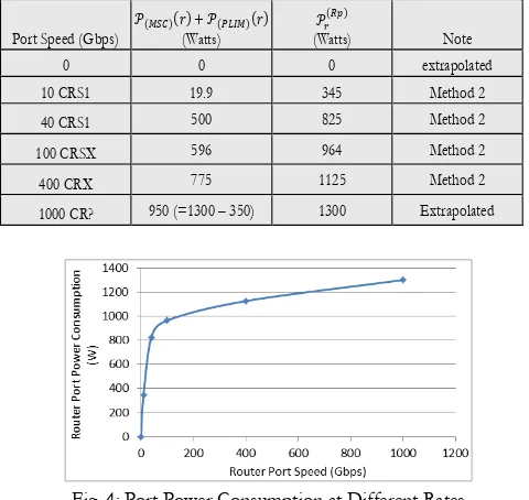
It is expected that in 2020 line rates of 1000 Gbps will be commercially available on most routers. In order to fully utilize the robustness of mixed line rate in 2020, it is necessary to establish the power consumption of a 1000 Gbps router port. Using the commercially available power consumption values determined using Method 2, we were able to extrapolate the power consumption of a 1000 Gbps port. We first determined the power consumption of the 10 Gbps port on the CRS-1 chassis and then plotted all the known power consumption values at the different data rates from Table III in Fig. 4.

Table III: Port Power Consumption at Different Rates

Fig. 4: Port Power Consumption at Different Rates

2. Equipment Power Consumption Improvements in 2020

The 2020 equipment power consumption is evaluated in two scenarios; a business as usual scenario (BAU) and a business as usual with GreenTouch improvements scenario (BAU+GT). The BAU equipment power consumption is obtained by only applying expected energy efficiency improvements due to advanced CMOS technologies. However, predicting future scaling of CMOS is probably harder now than it has ever been. CMOS has moved out of "Classical (geometrically driven) Scaling” where performance was driven by new litho tools leading to smaller transistors that could be easily projected. It is now in the era of "Equivalent Scaling” where performance is driven by changes in technology such as strained silicon [31], high-K/metal gate [32], multi-gate transistors [33] and integration of germanium and compound semiconductors [34]. There is some geometric scaling but this is tapering off and by 2020 will be irrelevant. Since each of these new techniques represents a discrete jump rather than a smooth scaling, it is much more difficult to project. Beyond the 2020 time window it gets more challenging. By 2028 the equivalent scaling will be

over and the future transistor count scaling will be through 3D stacking [35] and this does not bring direct device level energy benefits. We are seeing 3D scaling today and it may modify the path by 2020 as well. Taking these factors into consideration and the work presented in [36] and [37], improvements are expected to be around 0.78x (22%) per year for processing (logic) and 0.9x (10%) per year for interconnects. These improvements are also not expected to be the same for all the areas in the network since the constraints are different. For example, in the core network, the chips are often performance limited whereas at the edge they may be power limited and hence design choices maybe different. The split of power between logic and interconnects make the usual Moore’s law number that is widely quoted and was used in [3] and [4] as 0.88x (12%) improvement per year. Table IV shows the various improvement factor ratios used to project the power consumption values.

Table IV: Improvement Factors

The following therefore are the expected improvements for each category of equipment in the year 2020;

a) Routers:

An assumption has been made for routers, where processing and interconnects consume the same amount of power. If

therefore processing improves by per year and

interconnects by per year, router BAU improvement from 2010 to 2020 will be;

(62)

where is the ratio of the split in power consumption between interconnects and processing. In this case,

GreenTouch initiatives save power in interconnects by implementing optical interconnects by a factor of and saves processing power by matching /adapting processor capability to packet size by a factor of . At present, router processors are designed for worst case to handle small sized packets of 64 bytes (acknowledgement packets, the smallest packets) although a large number of packets is sized 1500 bytes (the maximum Ethernet packet size), ie bi-modal packet size distribution. The average packet size is around 500 to 600 bytes. Therefore, the overall improvement in a router in 2020 as a result of GreenTouch initiatives (BAU+GT) is;

b) Transponders:

The DSP accounts for 50% of the power consumption in transponders and the other 50% is due to other power consuming elements [38]. The 50% DSP is made up of 75% logic and 25% interconnects. Therefore, a transponder is;

logic, interconnects and

other components (electronics and very little optics). In the same way as the routers, the logic power consumption will improve by and the interconnects by . The other non DSP components which are mostly electronics will improve by which is Moore’s law only. The BAU improvements expected in 2020 in transponders is therefore:

By the same measure as in routers, the BAU+GT improvement will come from the optical interconnects that Port Speed (Gbps)

+

(Watts) (Watts) Note

0 0 0 extrapolated

10 CRS1 19.9 345 Method 2

40 CRS1 500 825 Method 2

100 CRSX 596 964 Method 2

400 CRX 775 1125 Method 2

1000 CR? 950 (=1300 – 350) 1300 Extrapolated

Factor Description Value

Annual improvements in logic 22% per year 0.78 Annual improvements in interconnects 10% per year 0.9

Usual Moore’s law of 12% per year 0.88 Packet size adaptation improvement in routers 0.2

will reduce the interconnects power by a factor of . An additional GreenTouch initiative that employs dynamic volatage and frequency scaling in transponder DSPs [38], [39] will reduce power consumption by a factor .

The transponder BAU+GT improvements expected in 2020 becomes:

Regenerators are expected to follow the same trend as transponders. EDFAs will only improve according to Moore’s law and it is not expected that they will have any further improvements because the non-electronics parts of EDFAs are mostly made up of optics. Optical switches will stay the same for a BAU network in 2020 but improvements of the order of 0.1x are expected in a BAU+GT network according to the work in [40]. Table V shows the power consumption values of various components that have been used for the MILP model for a 2010 network and a 2020 BAU and BAU+GT network worked out according to the methods aforementioned. Power usage effectiveness (PUE) values of 2 and 1.5 have been used for the 2010 and 2020 networks respectively.

Table V: Power Consumption Values

V.

TRAFFIC MODELLING FOR 2010 AND 2020

NETWORKS

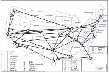
The impact of the different energy saving techniques is evaluated over a US continental network depicting the city locations of the AT&T network as shown in Fig. 5. The network consists of 25 nodes and 54 bidirectional links. This network was chosen because it is more representative of a realistic core network compared to the NSFNET, of 14 nodes and 21 bidirectional links, considered in our previous GreenMeter study [3]. Since the chosen network covers the entire US, different parts of the network fall in different time zones. The traffic used here is with respect to Pacific Standard Time (PST). We have selected nodes 1, 5, 8, 11, 13, 22 and 25 to host data centres according to the AT&T data centre map [43].

Fig. 5: Network Topology Used

The Cisco Visual Network Index (VNI) [38] provides a forecast of various categories of global IP traffic in exabytes per month. Given the traffic in exabytes per month (EBM), the daily traffic in Gb/s can be calculated as follows:

(66)

Given the daily traffic, the traffic demands between node (city) pairs in the network are obtained based on a modified gravity model where the traffic between nodes is proportional to the product of the population of the two nodes and independent of the distance between them. This form of the gravity model is typical for Internet traffic [45] The traffic matrix generated is then used together with the diurnal traffic cycle to produce traffic matrices for the network at different times of the day. Traffic from all the group one nations has been included in the forecast. Fig. 6 shows the daily network traffic at different times of the day for years 2010 and 2020 [14], [15], [16]. The projection for the 2020 traffic shows an increase by a factor of 12 compared to 2010 traffic. Also note that the 2020 diurnal cycle is much deeper than the 2010 cycle. This is due to two effects. Firstly, a higher Cisco VNI projected video consumption at peak evening hours in 2020 compared to 2010 attributed to growth in on demand services. Secondly due to a higher projected penetration of high definition video in 2020 compared to 2010.

We have also considered the data center to data center (DC-DC) traffic generated due to the creation of distributed cloud data centers. Distributed data centers need to talk to each other to synchronize the replicated content with the central cloud data center (i.e. the cloud data center that the model will choose if it was to build only one cloud data center) and to connect virtual machines located in different clouds. We have assumed that the DC-DC traffic is linearly related to the number of cloud data centers created in the network, and that half of the total traffic is due to the content in the clouds and the other half is due to virtual machines. If for example the model builds only one cloud, then the DC-DC traffic in the network is equal to zero. If more than one cloud data center is built in the network, that is, , the synchronization traffic for content between the central cloud data center and each cloud data center, , is given as:

(67)

(a)

(b)

Fig. 6: Daily Traffic Demand for (a) 2010 and (b) 2020 Networks 0

20 40 60 80 100 120 140 160 180

0 2 4 6 8 10 12 14 16 18 20 22

Tr

af

fi

c

in

T

b

p

s

Time of the Day

2010 Traffic

2010

0 500 1000 1500 2000 2500 3000

0 2 4 6 8 10 12 14 16 18 20 22

Tr

af

fi

c

in

T

b

p

s

Time of the Day 2020 Traffic

Table VI: Traffic Types

Note that is not a function of . This is because of the assumption that linearly increases at a constant slope, , and is zero if there is only one built cloud, i.e.

. Therefore, is a linear function of ( ) and the latter is cancelled by the denominator of (67). The factor of 2 in the denominator of the above equation is attributed to the fact that traffic due to content is half the total DC-DC traffic in the network. Fig. 7(a) shows the DC-DC traffic between cloud data centers for for content

distribution. Given the total DC-DC traffic

Tbps, the traffic between each cloud data center and the central cloud data center can be calculated from equation (67) as 2228.25 Tbps.

Fig. 7: Illustrative Example of DC-DC Traffic, n=3 (a) Content Distribution (b) Virtual Machine Placement

The DC-DC traffic due to virtual machines is considered to exist between all cloud pairs. If the model decides to build cloud data centers, that is, , the bidirectional traffic between a cloud pair due to virtual machines, , is given as:

(68)

Fig. 7(b) shows this traffic for scenario where the total DC-DC traffic is 8913 Tbps. From equation (68) the bidirectional traffic between a cloud pair is 742.75 Tbps. Table VI shows the values of the various traffic strands that have been considered as inputs to the MILP model.

VI. MILP MODEL RESULTS AND ANALYSIS

In this section, we present and discuss the power consumption of the AT&T network under the different energy efficiency techniques investigated in this paper which represent a 2020 network.

For content distribution and VM placement, users are uniformly distributed among the nodes and the total number of users in the network fluctuates throughout the day between 200,000 and 1,200,000. For the virtual network embedding service, clients are distributed across the entire network. A total of 50 virtual network clients have been considered. The number of clients from each city is dependent on the city’s population. The virtual network clients are considered to generate traffic in the network that is equivalent to 50% of the business internet traffic. The number of virtual nodes per virtual network request (VNR) from a client is uniformly distributed between 1 and 5.

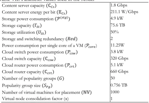
Each virtual node has a processing requirement in terms of virtual cores which are uniformly distributed between 500 and 3000 cores. The requests once accepted into the network stay in the network for a 2 hour slot after which they are torn down and adjusted according to the new arriving demands. A fully provisioned request should be able to provide processing resources in any cloud data center as well as bidirectional traffic resources from the clients’ location to any cloud data center. In order to achieve load balancing, virtual nodes belonging to the same VNR are not allowed to be embedded in the same cloud data center. Table VII shows the values of the parameters that have been used for the model. The power consumption in data centers due to VMs is considered to be proportional to the number of VM cores used.

Table VII: Parameter values used in the Model

Content server capacity 1.8 Gbps

Content server energy per bit 211.1 W/Gbps

Storage power consumption 4.9 kW

Storage capacity 75.6 TB

Storage utilization 50%

Storage and switching redundancy 2

Power consumption per single core of a VM ( ) 11.25W

Cloud switch power consumption 3.8 kW

Cloud switch capacity 320 Gbps

Cloud router power consumption 5.1 kW

Cloud router capacity 660 Gbps

Number of popularity groups 50

Popularity group size 0.756 TB

Number of virtual machines for placement 1000

Virtual node consolidation factor ( ) 1

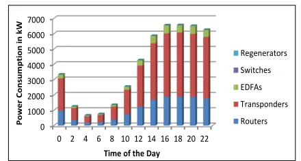
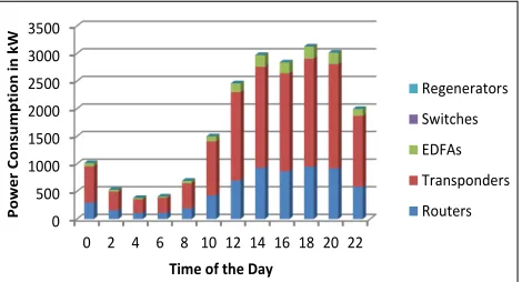
In the following results, we show the power consumption of individual components that make up the core network. Fig. 8 shows the reference case which is the power consumption of the AT&T network under 2010 traffic, 2010 components and a 2010 network design where the network is dimensioned for maximum traffic and the non-bypass approach is implemented. Components in the network do not adapt their power usage as the traffic varies, hence the flat trend in Fig. 8. The protection paths are also kept in active state together with the working paths. The major contribution to the total power consumption in 2010 is due to the routers and then followed by transponders.

A. 2020 Power Performance with BAU and BAU+GT Components, Idle Protection, Bypass and Sleep Techniques

Fig. 9 shows the power consumption in a 2020 network under the BAU scenario. Here, the total traffic in the network has increased to the levels shown in Fig. 6. The components’ power consumption in the network is also reduced by BAU factors (due to Moore’s law) presented in Table V. The overall network power consumption in 2020 due to equipment improvement is reduced by factor of 4.23 when compared to the 2010 network. Note that this reduction and other reductions comparing 2020 network to 2010 network reported in this section takes into account that the 2020 traffic increase by a factor of 12 compared to the 2010 traffic (i.e. the energy per bit in 2020 is reduced by factor of 4.23 compared to that in 2020). The network power consumption considering improved components in 2020 due to GreenTouch initiatives (BAU+GT) is shown in Fig. 10. The network power consumption has been reduced by a factor of 20 compared to 2010. The routers power consumption is reduced more than the transponders and as a result we see an almost equal contribution to the overall power consumption in the network from both transponders and routers.

One of the GreenTouch contributions to reducing power consumption in 2020 is to put all the protection paths to sleep while the working paths are active. The savings when using this

Central Cloud 1 Cloud 3 Cloud 2

2228.25 Tbps

2228.25 Tbps

Central Cloud 1 Cloud 3 Cloud 2

742.75 Tbps

742.75 Tbps

742.75 Tbps

742.75 Tbps 742.75 Tbps

742.75 Tbps

measure are reflected in Fig. 11. A reduction of 1.96x is achieved through this measure. Optical bypass where router ports at intermediate nodes are bypassed using the optical layer [4] and sleep techniques where unused router ports, transponders and regenerators are put to sleep are implemented in Fig. 12. Therefore, the power consumption follows the traffic variation throughout the day and a saving of 2.13x is achieved.

Fig. 8: Power Consumption of the Original AT&T Topology, 2010 Components, 40Gbps, non-bypass and Active Protection

Fig. 9: Power Consumption of the Original AT&T Topology, 2020 BAU Components, 40Gbps, non-bypass and Active Protection

Fig. 10: Power Consumption of the Original AT&T Topology, 2020 BAU+GT Components, 40Gbps, non-bypass and Active Protection

Fig. 11: Power Consumption of the Original AT&T Topology, 2020 BAU+GT Components, 40Gbps, Non-bypass and Idle Protection

Fig. 12: Power Consumption of the Original AT&T Topology, 2020 BAU+GT Components, 40Gbps, Bypass, Sleep and Idle Protection

B. 2020 Power Performance with Mixed Line Rates (MLR) and Topology Optimization

Optical networks with mixed line rates (MLR) have been proposed in [6] and [7] as a flexible architecture to efficiently support a heterogeneous range of applications in the core network. MLR mitigates the waste of optical bandwidth and

creates potential for energy savings. The other consideration is that router ports (Fig. 3), transponders and regenerators power consumption, does not scale linearly with data rates. Therefore, MLR uses an optimal combination of router ports, transponders and regenerators that minimizes the power needed to serve a given demand. For the 2020 network, four line rates, 40Gbps, 100Gbps, 400Gbps and 1000Gbps have been considered. Fig. 13 shows the network power consumption in 2020 implementing MLR. Routers have benefited from the (observed and extrapolated) saturation behavior that occurs as the data rates increase as can be seen in Fig. 4. Therefore the routers power consumption has been reduced the most. Transponders power consumption has not shown a significant reduction because at higher data rates, the transponder consumes a considerable amount of power. This behavior is expected in transponders because at higher data rates, transponders with very long reaches (i.e. in core networks) will have higher order modulation and will operate in the 1550nm window. This means that the signals will be subject to heavy forward error corrections (FEC) which will incur a power consumption penalty. We would therefore expect long reach high capacity transponder ports to consume more power than short reach high capacity router ports. The total network power consumption reduction due to MLR is 1.2x.

Optimizing the physical topology for power minimization in IP over WDM networks was investigated in [8]. We use the same techniques here to optimize the topology of the 2020 AT&T network for optimal power consumption. Fig. 14 shows the optimal topology obtained.

Fig. 13: Power Consumption of the Original AT&T Topology, 2020 BAU+GT Components, MLR, Bypass, Sleep and Idle Protection

Fig. 14: Optimized 2020 AT&T Topology BAU+GT Components, MLR, Bypass, Sleep and Idle Protection

Fig. 15: Power Consumption of the Optimized AT&T Topology, 2020 BAU+GT Components, MLR, Bypass, Sleep and Idle

Protection 0 10000 20000 30000 40000 50000

0 2 4 6 8 10 12 14 16 18 20 22

Po w er C on su m pt io n in k W

Time of the Day (Hours)

Regenerators Switches EDFAs Transponders Routers 100000 105000 110000 115000 120000 125000 130000

0 2 4 6 8 10 12 14 16 18 20 22

Po w er C on su m pt io n in k W

Time of the Day

Regenarators Switches EDFAs Transponders Routers 0 5000 10000 15000 20000 25000 30000

0 2 4 6 8 10 12 14 16 18 20 22

Po w er C on su m pt io n in k W

Time of the Day

Regenarators Switches EDFAs Transponders Routers 0 2000 4000 6000 8000 10000 12000 14000 16000

0 2 4 6 8 10 12 14 16 18 20 22

Po w er C on su m pt io n in k W

Time of the Day

Regenerators Switches EDFAs Transponders Routers 0 2000 4000 6000 8000 10000 12000

0 2 4 6 8 10 12 14 16 18 20 22

Po w er C o n su m p ti o n in k W

Time of the Day

Regenerators Switches EDFAs Transponders Routers 0 2000 4000 6000 8000 10000

0 2 4 6 8 10 12 14 16 18 20 22

P o w e r C o n su m p ti o n in k W

Time of the Day

Regenerators Switches EDFAs Transponders Routers 0 1000 2000 3000 4000 5000 6000 7000

0 2 4 6 8 10 12 14 16 18 20 22

P o w e r C o n su m p ti o n i n k W

Time of the Day

The minimum nodal degree in the optimized topology was kept at 2 to ensure that nodes are not totally isolated from the rest of the network in case of a single link failure. The optimal topology was obtained without any limit on the total number of links in the network. The optimal topology has a total of 193 links compared to the original topology which has a total of 54 links. Our previous results in [8], when no limit was set on the number of links, the optimal topology was a full mesh. However, in this work we have considered MLR and much longer distances between nodes which require regeneration. Since the power consumption of a regenerator is about twice the power consumption of a transponder, it becomes more energy efficient for traffic flows to pass through intermediate nodes using optical bypass instead of travelling through a longer direct link where one or more regenerators would be required. Fig. 15 shows the power consumption in a 2020 AT&T network with an optimized topology. The network power consumption reduction due to topology optimization is 1.43x.

Fig. 16 shows the power consumption of the 2020 AT&T network implementing the different distributed clouds discussed in this paper. Distributed clouds reduce the journeys up and down the network to access content and therefore reduce power consumption. We establish the optimal number of clouds to construct where to locate them and which cloud should contain which object based on popularity. In virtual machine slicing, we replicate smaller slices of virtual machines in the network without changing the overall power consumption in servers thereby reducing the overall power consumption in the network. We however limit the extent of slicing in order to meet the quality of service thresholds. In network virtualization, we consolidate the use of resources in the network by optimally embedding virtual network nodes and links such that they form minimal number of hops in the network. Virtual network requests from the same location but from different clients are co-located and the traffic they generate is groomed together to minimize network power consumption. When all these approaches are implemented a saving of 2.19x in network power consumption is achieved.

The overall saving in network power consumption considering all the approaches in 2020 compared to the 2010 network are 315x. Fig. 17 shows the network efficiency trend for the 2010 and 2020 network considering the various approaches investigated by GreenTouch. The energy efficiency of the 2010 network is 2774 kbps/W which translates to 360nJ/b.

Fig. 16: Power Consumption of the Optimized AT&T Topology, 2020 BAU+GT Components, MLR, Bypass, Sleep, Idle Protection

and Distributed Cloud for Content Delivery, VM Slicing and Network Virtualization

Fig. 17: The Energy Efficiency of both the 2010 and 2020 AT&T Network Under Different Energy Savings Techniques

VII. EXPERIMENTAL DEMONSTRATION OF THE

ENERGY EFFICIENT CONTENT DISTRIBUTION APPROACH IN IP/WDM

NETWORKS

In this section we introduce an experimental demonstration that illustrates the feasibility of energy efficient content distribution in IP/WDM networks.

1. Experimental Setup:

The experiment emulates the NSFNET network topology depicted in Fig. 18. It consists of 14 IP/WDM nodes connected by 21 bidirectional optical links. Each NSFNET node is emulated using a Cisco 10GE, SG 300-10, Layer 3 switch router. Each router is connected to an HP ProLiant DL120G7 server where content servers and clients are implemented. The routing table in each router is statically configured where the next hop is calculated based on shortest hop paths. Table VIII summarizes the details of the hardware we used in our experiment. Fig. 19 shows the routers and switches placed in two racks and connected to each other to form the NSFNET topology.

Fig. 18 The NSFNET Network With Link Lengths In km

We implemented the software entities (servers and clients) using Python 2.7 based on the asynchronous event driven TWISTED library. We used the MATLAB plotting library, Matplotlib [49] to display the result instantly. The results obtained from the experiment are updated every 1 second on the monitor screen. The traffic demands between network node pairs are calculated based on the clients’ locations and their download rate obtained from the servers. Given this demand distribution, we calculate network power consumption based on the number of hops between servers and clients, as will be explained below.

Table VIII: Demo Hardware Components

Hardware Number Type Specifications

Router 14 Cisco SG

300-10

10 GE ports [47]

Server 14 HP ProLiant

DL120G7

Intel® Xeon® E3, RAM 4GB,

HD250GB [48]

0 500 1000 1500 2000 2500 3000 3500

0 2 4 6 8 10 12 14 16 18 20 22

P

o

w

e

r

C

o

n

su

m

p

ti

o

n

i

n

k

W

Time of the Day

Regenerators

Switches

EDFAs

Transponders

Routers

0 0.1 0.2 0.3 0.4 0.5 0.6 0.7 0.8 0.9

1 2 3 4 5 6 7 8

Ef

fic

ie

nc

y

(G

bp

s/

W

)

1. Original AT&T Topology, 2010 Components, 40Gbps, non-bypass and Active Protection 2. Original AT&T Topology, 2020 BAU Components, 40Gbps, non-bypass and Active Protection 3. Original AT&T Topology, 2020 BAU+GT Components, 40Gbps, non-bypass and Active Protection 4. Original AT&T Topology, 2020 BAU+GT Components, 40Gbps, Non-bypass and Idle Protection 5. Original AT&T Topology, 2020 BAU+GT Components, 40Gbps, Bypass, Sleep and Idle Protection 6. Original AT&T Topology, 2020 BAU+GT Components, MLR, Bypass, Sleep and Idle Protection 7. Optimized AT&T Topology, 2020 BAU+GT Components, MLR, Bypass, Sleep and Idle Protection 8. Optimized AT&T Topology, 2020 BAU+GT Components, MLR, Bypass, Sleep, Idle Protection and