This is a repository copy of Calculation of confidence intervals for a finite population size. White Rose Research Online URL for this paper:
http://eprints.whiterose.ac.uk/138616/ Version: Accepted Version
Article:
Julious, S.A. orcid.org/0000-0002-9917-7636 (2018) Calculation of confidence intervals for a finite population size. Pharmaceutical Statistics. ISSN 1539-1604
https://doi.org/10.1002/pst.1901
This is the peer reviewed version of the following article: Julious SA. Calculation of
confidence intervals for a finite population size. Pharmaceutical Statistics. 2018, which has been published in final form at https://doi.org/10.1002/pst.1901. This article may be used for non-commercial purposes in accordance with Wiley Terms and Conditions for
Self-Archiving.
eprints@whiterose.ac.uk https://eprints.whiterose.ac.uk/ Reuse
Items deposited in White Rose Research Online are protected by copyright, with all rights reserved unless indicated otherwise. They may be downloaded and/or printed for private study, or other acts as permitted by national copyright laws. The publisher or other rights holders may allow further reproduction and re-use of the full text version. This is indicated by the licence information on the White Rose Research Online record for the item.
Takedown
If you consider content in White Rose Research Online to be in breach of UK law, please notify us by
Calculation of Confidence Intervals for
a Finite Population Size
Abstract
For any estimate of response confidence intervals are important as they help quantify a plausible range of values for the population response. However, there may be instances in clinical research when the population size is finite but we wish to take a sample from the population and make inference from this sample.
Instances where you can have a fixed population size include when undertaking a clinical audit of patient records or in a clinical trial a researcher could be checking for transcription errors against patient notes.
In this paper we describe how confidence interval calculations can be calculated for a finite population. These confidence intervals are narrower than confidence intervals from population samples. For the extreme case of when a 100% sample from the population is taken there is no error and the calculation is the population response.
The methods in the paper are described using a case study from clinical data management
Key words
1
Introduction
For any clinical investigative outcome the calculation of confidence intervals is important [1]. A 95% confidence interval is defined as an interval, estimated from a sample, within which we are 95% certain that the true population value would lie. It therefore provides a range of responses around the estimate value of interest to assist in the assessment of the true effect [2].
There are instances in clinical research where we have a finite population size. For example, in a clinical audit in a general practice a researcher could review the records of patients with asthma in the practice to assess the asthma medications be prescribed for the patients. Here the population is all the patients with asthma in the practice. Thus, the research could review the clinical records for all these patients or simply take a sample of all these patients with the knowledge that this will provide sufficient information for the research question [3]. This sample will in turn provide an estimate for the parameters of interest for the population – which here is all the patients with asthma in the practice.
The same situation arises in clinical trial research. For example, on a site visit for a multi-centre trial a researcher could check for transcription errors between data entered onto the case record form against the clinical records. Similarly, for a school based intervention where school absences for the children is the primary outcome a researcher could check what is recorded for the trial against the original data source – the school registers. In both these examples the population is the study population and to get an estimate of the number of errors a researcher could review all the records for all the people in the trial or take a sample and from this get an estimate of the population response.
In this paper we will first describe standard methods for confidence interval estimate before extending this for finite population. We will then apply methodologies with a motivating example taken from clinical data management
2
Motivational Example
In the planning of a quality control (QC) check of a database for non-critical data a
priori it is imagined that an error rate that could be observed is 0.5%.
In doing this QC check we could 100% sample all the data in the database to assess the proportion of errors. As this is non-critical data there may be a wish to save resource by taking a sample and estimate the proportion of errors from this. Then, only if this sample gives cause for concern take a bigger sample from the database.
and make any assessment from the upper bound from the CI for the worst case estimate of error rate.
2.1 Standard Methods Ignoring the Finite Population Size
2.1.1 Normal Approximation Confidence Intervals
If k events are observed in n observations such that the event rate can be estimated to be p=k/n. Then the 95% confidence interval for p can be estimated from
(1)
n p p Z
p 1 /2 (1 ) −
± −α .
Where is the level of statistical significance ( =0.05 would give 95% confidence
intervals) and Z the standard Normal values for .
1.1.1. Beta Distribution Confidence Intervals
For the case study the error rate is expected to be very low. Thus, to calculate confidence intervals for a binary response we will make use of the link between the Binomial and Beta distribution. The utility of calculating confidence intervals using a Beta distribution in the context of this paper is that the methodology can be used if the event of interest is very rare – such as assessing the number of errors in a data base.
Using a Beta distribution the lower bound for a confidence interval is defined as [4-6]
(2) 1−BETAINV
(
1−α 2,n−k+1,k)
,and upper as [4-6]
(3) BETAINV
(
1−α 2,k+1,n−k)
.As with the Normal case before: α is the level of statistical significance, k the number of events observed and n the sample size in the investigation. BETAINV
( )
• refers to the cumulative distribution function of a Beta distribution. The upper and lower bounds calculate from (2) and (3) will provide range of plausible values that the population prevalence is likely to be within.in most statistical packages, or using spreadsheet packages such as SAS or even Excel. Indeed the BETAINV
( )
• notation given in this paper is taken from Excel.Note (2) works for all values except when k=0. Here the lower bound would be fixed at 0 (or 0/n). Also, (3) works for all values except when k=n. Here the upper bound would be fixed at 1 (or k/n).
2.1.2 One Tailed or Two Tailed?
The question of whether to calculate one or two tailed confidence intervals is not straightforward [8]. For confidence intervals it depends on whether you wish to provide an estimate of the plausible range for the true value (two tailed) or a value, which you are confident that the true value will not exceed (one tailed).
For rare events it is often one tailed confidence that that you are interested in such that a one-tailed 1-α % bound is estimated from
(4) BETAINV
(
1−α,k+1,n−k)
.This one tailed confidence interval will give you an upper bound for the prevalence for a given number of events (k) in n subjects that you would be 1-α% confident that the population prevalence is unlikely to be greater than.
Note there is a school of thought that when computing a one tailed test you should set your significance level at half that of a two sided test [9]. In this paper we shall use the same level of significance for both two and one-sided tests.
2.1.3 Worked Example Ignoring the Finite Population Sample
In the planning of a QC of a database for non-critical data we imagined that an error rate we would see would be 0.5%. We are mainly interested in ruling out what the error rate could be worst case and so we wish to calculate simply a one tailed confidence interval for the upper bound using a Beta distribution.
Table 1. Confidence intervals for a proportion of observed errors in a QC for different sample sizes. Number of Errors Sample Size Point Estimate (%)
One Tailed Upper 95% CI (%)
1 200 0.50 2.35
3 600 0.50 1.29
5 1000 0.50 1.05
10 2000 0.50 0.85
30 6000 0.50 0.68
40 8000 0.50 0.65
50 10000 0.50 0.63
125 25000 0.50 0.58
250 50000 0.50 0.56
500 100000 0.50 0.54
1250 250000 0.50 0.52
2.2 Methods for Accounting for Finite Populations
2.2.1 Normal Approximation
To calculate confidence intervals for a binary response to account for the fact that our sample size n is in fact drawn from a finite sample size N we can estimate the upper and lower bound of the confidence interval, using a Normal approximation, to be [10]
(5) 1 ) 1 ( 2 / 1 − − − ± − N n N n p p Z
p α .
It is worth comparing he result (5) with (1) given earlier – for a standard 95% confidence interval estimate. The additional right hand term has the effect of making the confidence interval narrower. Such that for the extreme case of n=N, where a 100% sample is take, there is no error as p is the population estimate
2.2.2 Beta Distribution
If a Beta distribution is to be used to estimate the confidence interval then we can estimate the lower bound of the confidence interval to be [10]
(6)
(
(
)
)
1 , 1 , 2 1 1 1 1 − − + − − − + − − − N n N k k n BETAINV N n N n k α ,
and upper as [10]
(7)
(
(
)
)
1 , 1 , 2 1 1 1 − − − + − + − − − N n N k n k BETAINV N n N n k α .
the sample from which the estimate is obtained is actually a fraction, (n/N), of the population sample size, N.
It is easier to think in terms of the proportion of the finite sample drawn r defined as
(8)
N n r= .
Hence, using r we can estimate the lower bound of the confidence interval to be
(9)
(
(
)
)
r n n r k k n BETAINV r n n r n k − − + − − − + − −
− (1 ) 1 1 2, 1, (1 )
1 α ,
and upper as
(10)
(
(
)
)
r n n r k n k BETAINV r n n r n k − − − + − + − −
− (1 ) 1 2, 1, (1 )
1 α .
From
(7) a one tailed confidence interval for the upper bound could be obtained from
(11)
(
(
)
)
1 , 1 , 1 1 1 − − − + − + − − − N n N k n k BETAINV N n N n k α ,
Which when written in terms of r becomes
(12)
(
(
)
)
r n n r k n k BETAINV r n n r n k − − − + − + − −
− (1 ) 1 , 1, (1 )
1 α .
From now on in the paper the concentration will be on methods using the Beta distribution.
Note again, as for the Normal approximation earlier, if n=N then all the confidence intervals return the point estimate, k/n, as the best estimate.
2.2.3 Worked Example Accounting for the Finite Population Sample
For the same example earlier of a QC of a database of non-critical data suppose we are actually taking a 10% sample such that r=0.1. For the same sample sizes and anticipated QC error rates (0.5%) as previously Table 2 gives an illustration of possible assuming an error rate of 0.5% is observed in the data.
error rate of 0.5%. However, from the confidence intervals we can be 95% certain the error rate is no worse than 1.02%.
As we are interested in the estimate of how plausibly high could the error rate be –as this would necessitate action – we have only quoted the upper bound of one tailed confidence interval. Two tailed confidence intervals are not quoted as an estimate of how plausibly low the error rate could be is not of interest in the situation being described.
In the table we have repeated the results for the standard population estimate given earlier in Table 1. Note how the confidence interval for the finite population estimate are narrower than for the population estimate. This is because the population estimate result is calculated ignoring the valuable information that the sample size taken from a finite population. However, as the sample size increases the difference between the two methods becomes less pronounced.
A consequence of not using the fixed population estimate result could be that – based on the confidence interval – the error rate could be over stated which could lead to unnecessary further investigations
Table 2. Confidence intervals for a fixed proportion of observed errors in a QC for different
sample sizes as a proportion r=0.1 of the total sample size.
One Tailed Upper 95% CI (%) Number
of Errors
Sample Size
Point Estimate (%)
Standard Population Estimate
Fixed Population Size Estimate
1 200 0.50 2.35 2.26
3 600 0.50 1.29 1.25
5 1000 0.50 1.05 1.02
10 2000 0.50 0.85 0.83
30 6000 0.50 0.68 0.67
40 8000 0.50 0.65 0.63
50 10000 0.50 0.63 0.62
125 25000 0.50 0.58 0.57
250 50000 0.50 0.56 0.55
500 100000 0.50 0.54 0.54
1250 250000 0.50 0.52 0.52
A question to consider is whether a 10% sample is reasonable. As highlighted earlier if we had a sample size of 1000 an error rate of 0.5% then we would be able to say that we are confident that the true rate in the entire population is no less than 1.02%. Obviously if we sample a greater proportion of the population we would have a bigger sample size and hence greater precision.
[image:9.595.126.483.441.622.2]sample size of 10,000. We can see for this worked example that the precision in the estimates falls quickly until about 10% of the population is sampled. After this the precision falls at a slow rate until we have 100% of the population sampled.
Figure 1. Percentage precision by proportion sampled assuming a population sample size of
10,000 and a QC error rate of 0.5%
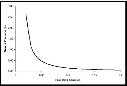
Figure 2 reconsiders the problem for the same population size and QC rate. This figure gives the gain in precision for every 0.01 increase in the proportion sampled. The gain in precision is measured as the absolute gain in precision measured and is assessed by estimating the as the width of the confidence interval from (11) for a given sample size n and taking this away from the confidence interval width for a sample size of n-1
[image:10.595.90.503.201.434.2]Figure 2. Gain in precision by proportion sampled assuming a population sample size of 10,000
and a QC error rate of 0.5%
2.2.4 Extending the Results
It should be noted that the results in this paper do not just apply to binary data. If a mean was to be estimated from a sample size of n, sampled from a finite population size of N patients then the Normal approximation results could in this paper could be extended. If the mean is estimated as x with corresponding standard error of σ/ n. Then, the 95% confidence interval can be estimated from
(13)
1
2 / 1
− − ± −
N n N n Z
x α σ
Where is the level of statistical significance ( =0.05 would give 95% confidence
intervals) and Z the standard Normal values for as before.
This result, like for binary data, is an extension of a population estimate confidence interval of
(14)
n Z
3
Sample Size Calculations
So far we have simply discussed the sample size in terms of proportion of the database sampled. If what we wished to have was a point estimate estimated with an appropriate precision than this approach may require sample size greater than what is needed for a requisite precision. Unlike conventional sample size calculations, in which we calculate the number of patients required in a trial, in the context of clinical audit there is no ethical issues in having an over (or under) estimated sample size. However, it takes time to do a QC and an inappropriate sample size may lead to resource being used on the task which could be diverted to over sources.
In this sub section we will briefly describe sample size calculations that will give a required precision for a finite population.
3.1 Standard Methods Ignoring the Finite Population Size
To calculate the sample size to obtain a given precision, w, defined as half the wide for a confidence interval, for a two tailed confidence interval for a given anticipated response, p, we can use the following result
(15) w=
(
BETAINV(
1−α 2,k+1,n−k)
+BETAINV(
1−α 2,n−k+1,k)
−1)
/2We can iterate on n until we get a sample size with the requisite precision for a given p. We can estimate k from k=pn. This approach is known as a precision based approach to sample size estimation [13]
The equivalent result for a one tailed confidence interval would be
(16) w= BETAINV
(
1−α,k+1,n−k)
−k/n3.1.1 Worked Example Ignoring the Finite Population Sample
We wish to undertake a QC of a clinical database. We anticipate that the error rate will be around 0.5% but we wish to have an estimate of the response with precision also of 1%. The precision here would be assessed in terms of a one tailed 95% confidence interval. From (16) the sample size is estimated to be 432.
3.2 Methods for Accounting for Finite Populations
To calculate the sample size to obtain a given precision, w, for a given anticipated response, p, we can use the following result
(17)
(
(
1 2, 1,)
(1 /2, 1, ) 1)
(1 ) /2
− − + + − −
+ − + −
=
r n
n r k
k n BETAINV
k n k BETAINV
Where k=pn and we iterate on n until we get a sample size with the requisite precision for a given p.
The equivalent result for a one tailed confidence interval would be
(18)
(
(
)
)
r n
n r k
n k BETAINV
r n
n r n
k
− − −
+ − +
− −
− (1 ) 1 , 1, (1 )
1 α
Similarly for a two tailed confidence interval a sample size could be obtained from (16) and (18)
In these calculations only precision based calculations with 95% confidence intervals were considered. However the work can be extended to other trial objectives [13-14] and levels of confidence [15]
3.2.1 Worked Example Accounting for the Finite Population Sample
We now wish to repeat the QC worked sample of early. However, we now wish to take account of the fact that the clinical database has a finite size of 5,000 data points.
From (18) the sample size is estimate to be 409. This is a little less than 10% of the actual data base.
4
Discussion
In this paper confidence intervals were described for a response rate for a given sample size using the Beta distribution. We then extended the problem for the situation where we have a finite population size from which we are sampling. This approach led to more precise estimates. For the extreme case where the sample is the same as the population size there is no error in the estimate.
We recommend the approaches described on this paper be used if there is a finite population size from which a sample is being taken.
5
References
1. Gardner MK, Altman DG. Estimating with confidence BMJ 1988;296:1210-1.
3. Campbell MJ. Sample sizes in audit. British Medical Journal 1993;307:735-6
4. Daly L. Simple SAS Macros for the Calculation of Exact Binomial and Poisson Confidence Limits. Computational and Biological Medicine 1992;22:351-361.
5. Julious SA. Two-sided confidence intervals for the single proportion: comparison of seven methods (letter). Statistics in Medicine 2005 24:3383-4.
6. Newcomble, R.G. Two sided confidence intervals for the single proportion: comparison of seven methods. Statistics in Medicine 1998;17:857-72
7. Clopper, C.J. and Pearson, E.S. The Use of Confidence or Fiducial Limits Illustrated in the case of the binomial. Biometrika 1934;26:404-413.
8. Bland JM, Altman DG. Statistical notes: one sided and two sided tests of significance BMJ 1994;309:248
9. ICH E9. Statistical principals for clinical trials. September 1998.
10.Burstein, H. Finite Population Correction for Binomial Confidence Limits.
Journal of the American Statistical Association, 1975: 70(349) 67-69
11.Julious SA and Patterson SD. Sample sizes for estimation in clinical research. Pharmaceutical Statistics 2004;3:213-5.
12.Flight L and Julious SA. Practical guide to sample size calculations: non-inferiority and equivalence trials. Pharmaceutical Statistics 2016:15(1) 68-74
13.Flight L and Julious SA. Practical guide to sample size calculations: an introduction. Pharmaceutical Statistics 2016 15(1) 75-79
14.Flight L and Julious SA. Practical guide to sample size calculations: superiority trials. Pharmaceutical Statistics 2016 15(1) 80-89