Design Optimisation of a Magnetic Field Based Soft Tactile Sensor

(1)

Article

Design Optimisation of a Magnetic Field Based Soft

Tactile Sensor

Gregory de Boer1,* ID_{, Nicholas Raske}2_{, Hongbo Wang}3 ID_{, Junwai Kow}1_{, Ali Alazmani}1_, Mazdak Ghajari4, Peter Culmer1and Robert Hewson2

1 _{School of Mechanical Engineering, University of Leeds, Woodhouse Lane, Leeds LS2 9JT, UK;}

[email protected] (J.K.); [email protected] (A.A.); [email protected] (P.C.)

2 _{Department of Aeronautics, Imperial College London, South Kensington Campus, London SW7 2AZ, UK;}

[email protected] (N.R.); [email protected] (R.H.)

3 _{Center for Micro-BioRobotics, Istituto Italiano di Tecnologia, Viale Rinaldo Piaggio 34, 56025 Pontedera,}

Italy; [email protected]

4 _{Dyson School of Design Engineering, Imperial College London, 10 Princes Gardens, Kensington Princes}

Gardens, London SW7 1NA, UK; [email protected] * Correspondence: [email protected]; Tel.: +44-113-343-2206

Received: 28 September 2017; Accepted: 2 November 2017; Published: 3 November 2017

Abstract:This paper investigates the design optimisation of a magnetic field based soft tactile sensor, comprised of a magnet and Hall effect module separated by an elastomer. The aim was to minimise sensitivity of the output force with respect to the input magnetic field; this was achieved by varying the geometry and material properties. Finite element simulations determined the magnetic field and structural behaviour under load. Genetic programming produced phenomenological expressions describing these responses. Optimisation studies constrained by a measurable force and stable loading conditions were conducted; these produced Pareto sets of designs from which the optimal sensor characteristics were selected. The optimisation demonstrated a compromise between sensitivity and the measurable force, a fabricated version of the optimised sensor validated the improvements made using this methodology. The approach presented can be applied in general for optimising soft tactile sensor designs over a range of applications and sensing modes.

Keywords:tactile sensing; sensitivity; optimisation; magnetic fields; force measurement

1. Introduction

Tactile sensors enable robots to interact with humans and the environment with a high level of accuracy and enhance their abilities for dexterous manipulations. Concurrently, technical challenges

remain for soft tactile sensing systems to reach human-level performance [1]. Various physical

transducer mechanisms (e.g., resistive, capacitive, magnetic, piezoelectric, piezoresistive) have been

introduced to develop soft tactile sensors [2], with each design exhibiting their own set of advantages

and disadvantages. In general, resistive, capacitive, piezoelectric/piezoresistive tactile sensors have

high spatial resolution and performance [2,3], which are easy to implement on ultra-thin layers,

but they do not measure tri-axis force nor are they deformable. An encapsulation of soft skin on the working surface protects the sensor electronics and wires but this lowers the performance (in terms

of hysteresis, sensitivity, and bandwidth) and requires a complex fabrication process [4]. Optical

tactile sensors such as TACTIP [5] are durable and have high spatial resolution but are limited by

complex computation between inputs and outputs, high power consumption, and are difficult to use to

investigate a large sensing area. BioTac [6] is a bio-inspired fingertip which uses a conductive liquid to

transfer force to resistance and is capable of force, contact, temperature, and vibration measurements.

(2)

BioTac has been integrated into a range of robotic hand fingertip devices but remains expensive, complicated, and difficult to use over a large sensing area.

Originally presented by Clark [7], magnetic field-based tactile sensors use a remote sensing

approach which is inherently durable, deformable, low-cost, easy to fabricate, and easy to integrate

with existing robotic systems [8]. Wang et al. [9] introduced a comprehensive design methodology to

enable researchers from different disciplines to design high performance soft tactile sensors for specific

applications. A single element soft tri-axis tactile sensor, MagOne (Figure1a), was fabricated as a

prototype case study and achieved a force measurement resolution of approximately 1 mN with good repeatability and low hysteresis (3.4%). The performance of MagOne was comparable to commercial rigid force/torque sensors and cost about £10 to fabricate. All aspects, including geometry, fabrication, calibration, performance evaluation, advantages and disadvantages, were investigated to design a high performance soft tactile sensor based on the magnetic field measurement. However, given the complex relationship between magnetic field and force, the MagOne design was not optimised for the multiple design objectives associated with a range of diverse applications. The effect of a range of design variables (e.g., geometry and material properties) on the sensor performance needed to be characterised and from this an optimal design could be determined. Multi-element magnetic

field based soft sensors such as Tomo et al. [10] for soft-skin applications, de Oliveria et al. [11] for

multimodal sensing and Wang et al. [12] as an extension of MagOne have been recently established.

The optimisation principles developed in this work are also applicable to these cases, leading to a means of establishing improvements and optimising the performance of these sensors.

measurements. BioTac has been integrated into a range of robotic hand fingertip devices but remains expensive, complicated, and difficult to use over a large sensing area.

Originally presented by Clark [7], magnetic field-based tactile sensors use a remote sensing approach which is inherently durable, deformable, low-cost, easy to fabricate, and easy to integrate with existing robotic systems [8]. Wang et al. [9] introduced a comprehensive design methodology to enable researchers from different disciplines to design high performance soft tactile sensors for specific applications. A single element soft tri-axis tactile sensor, MagOne (Figure 1a), was fabricated as a prototype case study and achieved a force measurement resolution of approximately 1 mN with good repeatability and low hysteresis (3.4%). The performance of MagOne was comparable to commercial rigid force/torque sensors and cost about £10 to fabricate. All aspects, including geometry, fabrication, calibration, performance evaluation, advantages and disadvantages, were investigated to design a high performance soft tactile sensor based on the magnetic field measurement. However, given the complex relationship between magnetic field and force, the MagOne design was not optimised for the multiple design objectives associated with a range of diverse applications. The effect of a range of design variables (e.g., geometry and material properties) on the sensor performance needed to be characterised and from this an optimal design could be determined. Multi-element magnetic field based soft sensors such as Tomo et al. [10] for soft-skin applications, de Oliveria et al. [11] for multimodal sensing and Wang et al. [12] as an extension of MagOne have been recently established. The optimisation principles developed in this work are also applicable to these cases, leading to a means of establishing improvements and optimising the performance of these sensors.

(a) ₍_b₎

Figure 1. Photographs of the MagOne sensor designs. (a) As developed by Wang et al. [9]. (b) From the optimisation of sensitivity considered in this study.

This paper investigates the design optimisation of the MagOne sensor, for this purpose Finite element (FE) simulations were developed to determine the magnetic field and structural behaviour under load. Optimisation studies have been conducted using simulated results of magnetic fields [13,14] and compliant structures/mechanisms [15–17]; however, this paper is the first to apply design optimisation techniques in order to simultaneously address these interactions. Studies have also been conducted exploring the optimisation of soft sensors [18,19]. However, the sensors investigated have different operating modes to that of MagOne and the research outcomes did not produce optimised designs, but rather strategies for optimising the output sensing range by control of the input parameters. Genetic programming (GP) was used in this work as a metamodel to produce accurate relationships of the non-linear sensor response over the range of parameters investigated, which is a well-established approach in design optimisation [20]. The optimised designs presented were calculated using a combination of genetic algorithms (GAs) and heuristic solvers based on the relationships generated by GP; such solution procedures have been used previously for this purpose [21].

The motive for the optimisation was to improve the function of the sensor, as defined by its ability to accurately characterise an applied force. For the MagOne device this means a small change in applied load corresponds to a large change in the sensed magnetic field where the relationship between applied force and sensed magnetic field was defined as the sensitivity. The objective of the

Figure 1.Photographs of the MagOne sensor designs. (a) As developed by Wang et al. [9]. (b) From the optimisation of sensitivity considered in this study.

This paper investigates the design optimisation of the MagOne sensor, for this purpose Finite element (FE) simulations were developed to determine the magnetic field and structural behaviour

under load. Optimisation studies have been conducted using simulated results of magnetic

fields [13,14] and compliant structures/mechanisms [15–17]; however, this paper is the first to apply

design optimisation techniques in order to simultaneously address these interactions. Studies have also

been conducted exploring the optimisation of soft sensors [18,19]. However, the sensors investigated

have different operating modes to that of MagOne and the research outcomes did not produce optimised designs, but rather strategies for optimising the output sensing range by control of the input parameters. Genetic programming (GP) was used in this work as a metamodel to produce accurate relationships of the non-linear sensor response over the range of parameters investigated,

which is a well-established approach in design optimisation [20]. The optimised designs presented

were calculated using a combination of genetic algorithms (GAs) and heuristic solvers based on the relationships generated by GP; such solution procedures have been used previously for this

purpose [21].

(3)

applied load corresponds to a large change in the sensed magnetic field where the relationship between applied force and sensed magnetic field was defined as the sensitivity. The objective of the optimisation study was, therefore, to minimise sensitivity over a range of design variables. A second, and conflicting, objective was introduced to maximise the largest applied load that the sensor can characterise. This ensured that it will have a useful operating range. The design variables were selected to parametrise the geometry and material properties of the sensor, which can be altered as part of the fabrication process. Constraints on the measureable force, given as part of the sensor specification, were imposed and included in the design strategy. Shear loading conditions were investigated in order to optimise the sensor design over a representative range of operational displacements. The optimised designs

were subsequently validated by fabricating and experimentally testing the new sensor (Figure1b),

thus demonstrating the accuracy of the computational simulations and the improvements in sensitivity obtained by design optimisation.

The application of this approach to the optimisation of sensitivity subject to a load range (or conversely the optimisation of a sensing range subject to the load range, or a multi-objective optimisation process where both sensitivity and sensing range are considered in combination) can be readily applied to different sensing modalities, such as those based on capacitive based sensing where compression of a soft material and its mechanical response forms the basis of converting the

sensor deformation to the resulting force [22]. Indeed, the check for the uniqueness of response

and computational electro-mechanical characterisation of the response of a wide range of sensors

could potentially be characterised and optimised in terms of geometry [23] so long as a deterministic

computational model of the sensor can be derived [24–26]. The general method described in this paper,

where the sensor is parametrised by design variables which are then optimised based on numerical simulations and metamodels of the input/output response, is applicable to the design of a range of soft tactile sensors.

2. Materials and Methods

2.1. Sensor Concept

This work is focused on the optimisation of a magnetic sensor concept developed by Wang et

al. [9] which comprised of a 3D Hall module, a deformable elastomer body and an embedded magnet

as illustrated in Figure2a. The sensor, known as MagOne, worked by measuring the magnetic field

produced at the origin 0, by means of the induced electric field in the Hall effect module. By displacing the magnet from A, the change in magnetic field was identified and then the force applied was determined from knowledge of the mechanical behaviour of the elastomer under load.

Sensors 2017, 17, 2539 3 of 20

optimisation study was, therefore, to minimise sensitivity over a range of design variables. A second, and conflicting, objective was introduced to maximise the largest applied load that the sensor can characterise. This ensured that it will have a useful operating range. The design variables were selected to parametrise the geometry and material properties of the sensor, which can be altered as part of the fabrication process. Constraints on the measureable force, given as part of the sensor specification, were imposed and included in the design strategy. Shear loading conditions were investigated in order to optimise the sensor design over a representative range of operational displacements. The optimised designs were subsequently validated by fabricating and experimentally testing the new sensor (Figure 1b), thus demonstrating the accuracy of the computational simulations and the improvements in sensitivity obtained by design optimisation.

The application of this approach to the optimisation of sensitivity subject to a load range (or conversely the optimisation of a sensing range subject to the load range, or a multi-objective optimisation process where both sensitivity and sensing range are considered in combination) can be readily applied to different sensing modalities, such as those based on capacitive based sensing where compression of a soft material and its mechanical response forms the basis of converting the sensor deformation to the resulting force [22]. Indeed, the check for the uniqueness of response and computational electro-mechanical characterisation of the response of a wide range of sensors could potentially be characterised and optimised in terms of geometry [23] so long as a deterministic computational model of the sensor can be derived [24–26]. The general method described in this paper, where the sensor is parametrised by design variables which are then optimised based on numerical simulations and metamodels of the input/output response, is applicable to the design of a range of soft tactile sensors.

2. Materials and Methods

2.1. Sensor Concept

This work is focused on the optimisation of a magnetic sensor concept developed by Wang et al. [9] which comprised of a 3D Hall module, a deformable elastomer body and an embedded magnet as illustrated in Figure 2a. The sensor, known as MagOne, worked by measuring the magnetic field produced at the origin 0, by means of the induced electric field in the Hall effect module. By displacing the magnet from A, the change in magnetic field was identified and then the force applied was determined from knowledge of the mechanical behaviour of the elastomer under load.

(a) (b)

Figure 2. Cross-sectional sketch of the MagOne sensor. (a) Unloaded. (b) Loaded in both normal and shear directions.

Both normal (z-axis) and shear (r-axis) loading were considered, in which contact and friction

occurred between the upper and lower surfaces of the sensor and the rigid surfaces used for

indentation. Figure 2b illustrates normal and shear loading of the sensor due to a displacement =

u , u of the magnet, where = ∆ , ∆ is the distance between the magnet and the Hall effect

module, θ is the shear angle, = B , B is the magnetic field, = F , F is the force, and =

Γ , Γ is the sensitivity.

Figure 2.Cross-sectional sketch of the MagOne sensor. (a) Unloaded. (b) Loaded in both normal and shear directions.

Both normal (z-axis) and shear (r-axis) loading were considered, in which contact and friction

(4)

Figure2b illustrates normal and shear loading of the sensor due to a displacementu = (ur, uz)of

the magnet, where∆ = (∆r,∆z)is the distance between the magnet and the Hall effect module,

θis the shear angle,B = (Br, Bz)is the magnetic field,F = (Fr, Fz)is the force, andΓ = (Γr,Γz)is

the sensitivity.

The sensitivityΓ= (Γr,Γz)describes the magnitude of the derivatives of Frand Fzwith respect

to Brand Bz, as given in Equations (1) and (2). For the sensor design optimisation, the objective was

to minimise the change in the output of the sensorFfor any given change in the inputB, or in other

words to minimiseΓ. This ensured a robust sensor response, withFbeing less sensitive to noise in

the measuredB. Sensitivity was affected by the choices made in the design of the sensor such as the

geometry, material properties and component selection. In the concept developed here, the magnet and Hall effect module were chosen leaving the geometry and material properties as design variables. This decision was made because it provides the simplest means of varying parameters in the design while demonstrating the complexity of delivering an optimised sensor.

Γr=

s

∂Fr

∂Br

2

+

∂Fr

∂Bz

2

(1)

Γz=

s

∂Fz

∂Br

2

+

∂Fz

∂Bz

2

(2)

2.1.1. Sensor Mechanics

When the magnet was displaced byuthe distance between the Hall effect module and magnet∆

was changed. The relationship betweenuand∆was described by Equations (3) and (4),

uz=∆z+Hm−H−Hg (3)

ur =∆r (4)

where urand uzare the displacement components,∆zand∆rare the r and z distances from the magnet

to the Hall effect module, H is the sensor base height, Hmis the height of the magnet, and Hgis a

geometrical height for the sensor. At a given∆zthe reading of the Hall effect module became saturated,

this limit∆z,sat. defined the depth to which the indentation reached. The magnet was displaced linearly

with a non-dimensional variable t where 0≤t≤1, leading to Equations (5) and (6).

uz=t ∆z,sat+Hm−H−Hg (5)

ur =−t ∆z,sat+Hm−H−Hgtanθ (6)

The shear angleθwas limited to a value which was determined by an assumption derived from

the frictional characteristics of the sensor and indenting surfaces. The coefficient of frictionµ_fbetween

the sensor and indenting surfaces was defined by Equation (7),

Fr,slip

Fz,slip

=µ_f (7)

where Fr,slipand Fz,slipare the shear and normal force components at slip. Beyond this limit the

sensor material slips along the indenting surfaces, thus providing the limiting case under shear. Setting the ratio of displacement components equal to that of the force components at slip allowed an

approximation for the maximum shear angleθmaxto be determined, as described by Equation (8).

(5)

Structural mechanics simulations of the sensor under normal and shear loading, as described in

Section2.1.3, were conducted to ensure that this limit did not result in the elastomer material slipping

along the indenting surface. The variables t andθfully parameterised the range of displacements

urequired for a given sensor design. The space defined by the ranges of t andθis continuous and

bounded by t∈[0, 1]andθ∈[0,θmax].

2.1.2. Magnetic Field

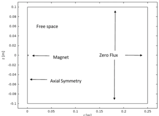
A model was developed to obtain the magnetic field in a fixed position and from whichBwas

obtained as a function of the magnet displacement. This approach was applicable because the structural mechanics of the sensor under load does not have an effect on the magnetic field distribution. A 2D

axially-symmetric cylindrical coordinate system was employed for developing the model becauseBis

independent of the orientation of the shear direction r. The solution forBwas described by Equation (9),

and Equation (10) described the relationship between the magnetized fieldHand magnetic scalar

potential V.

∇·B=0 (9)

H=−∇V (10)

In the space surrounding the magnet,Bwas described by Equation (11) and within the magnet it was

described by Equation (12),

B=µ₀µ_rH (11)

B=µ₀(H+M) (12)

whereµ₀is the permeability of free space,µ_ris the relative permeability, andMis the magnetisation

as governed by the magnet selection. A zero flux condition,n·B = 0 was applied at a boundary

far from the sensor (+100 Rm in r and±50 Hmin z), wherenis the surface normal vector and an

axial-symmetry condition was applied through the z-axis of the magnet centre (r = 0), as shown

in Figure3. The magnetic field was not affected by the material properties of the elastomer such

that the relative permeability of the elastomer and space surrounding the sensor isµ_r =1, i.e., no

shielding effect [27]. Using these operating and boundary conditions and solving Equations (9) and

(10) together with Equations (11) and (12) for V produced the magnetic fieldB. This was subsequently

assessed for all displacements and sensor designs by varying the distance between the magnet and assessment location.

Sensors 2017, 17, 2539 5 of 20

2.1.2. Magnetic Field

A model was developed to obtain the magnetic field in a fixed position and from which B was

obtained as a function of the magnet displacement. This approach was applicable because the structural mechanics of the sensor under load does not have an effect on the magnetic field distribution. A 2D axially-symmetric cylindrical coordinate system was employed for developing the

model because B is independent of the orientation of the shear direction r. The solution for B was

described by Equation (9), and Equation (10) described the relationship between the magnetized field

H and magnetic scalar potential V.

∇ ∙ = 0 (9)

= −∇V (10)

In the space surrounding the magnet, was described by Equation (11) and within the magnet it

was described by Equation (12),

= μ μ (11)

= μ + (12)

where μ is the permeability of free space, μ is the relative permeability, and is the

magnetisation as governed by the magnet selection. A zero flux condition, ∙ = 0 was applied at

a boundary far from the sensor (+100 Rm in r and ± 50 Hm in z), where n is the surface normal vector

and an axial-symmetry condition was applied through the z-axis of the magnet centre (r = 0), as shown in Figure 3. The magnetic field was not affected by the material properties of the elastomer

such that the relative permeability of the elastomer and space surrounding the sensor is μ = 1, i.e.,

no shielding effect [27]. Using these operating and boundary conditions and solving Equations (9) and (10) together with Equations (11) and (12) for V produced the magnetic field . This was subsequently assessed for all displacements and sensor designs by varying the distance between the magnet and assessment location.

Figure 3. Diagram of the magnetic field model.

2.1.3. Structural Mechanics

During indentation the sensor material underwent large strains leading to a requirement for nonlinear structural mechanics to be used to describe the problem. The elastomer used was a rubber-like silicone (Ecoflex 00-30) for which the stress-strain relationship was known to be hyperelastic [28]. For the sensor design an incompressible Neo-Hookean model was used to define the material properties. Wang et al. [9] demonstrated that this model was sufficiently accurate to describe the mechanical behaviour of MagOne under load. The incompressible Neo-Hookean model derives the

Figure 3.Diagram of the magnetic field model.

2.1.3. Structural Mechanics

(6)

a rubber-like silicone (Ecoflex 00-30) for which the stress-strain relationship was known to be

hyperelastic [28]. For the sensor design an incompressible Neo-Hookean model was used to define the

material properties. Wang et al. [9] demonstrated that this model was sufficiently accurate to describe

the mechanical behaviour of MagOne under load. The incompressible Neo-Hookean model derives the stress-strain relationship for the material from a strain energy density function W, as given in Equation (13),

W= G

2

λ2₁+λ2₂+λ2₃−3 (13)

where G is the shear modulus of the elastomer, andλ₁,λ₂,λ₃are the principle stretches. Stresses in the

material can be obtained by calculating the derivatives of W with respect to strains, which themselves relate to the principle stretches. Variation of G can be achieved by changing the silicone used in the fabrication process, thus varying the elastomer stiffness. A steady-state assumption is made in the analysis such that no dynamic behaviour (viscoelasticity or inertia) was modelled. This was confirmed

by experimental validation of the sensor showing 3.4% hysteresis [9].

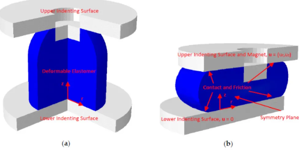
In order to model indentation of the sensor to include both normal and shear loading a full three-dimensional description of the sensor was required, this was because as the sensor deformed in shear the shape of the sensor was not axially-symmetric, and thus, the dimension cannot be reduced as in the case for the magnetic field calculation. The magnet was modelled as a rigid body which

was rigidly connected to the elastomer material surrounding it, and was displaced by ur, uzin the

r-axis andz-axis, respectively, to produce normal and shear loads. The base of the elastomer was

fixed such that the displacement was constrained to zerou = 0, and the sides of the sensor were

allowed to freely deform. A symmetry condition was specified in the plane to which shear was applied. Contact mechanics was considered to model the interaction between the freely deforming surfaces of the elastomer and the indenting surfaces, which were themselves considered rigid bodies. Friction was generated during indentation and this effect was modelled by specifying a coefficient of friction

µ_ffor the contact. Figure4a,b show the structural model of the sensor for when it was unloaded

and loaded, respectively. Equation (13) was solved according to these operating and boundary conditions to give the stress distribution under load over the required ranges of displacement and

sensor designs. The value ofF= (Fr, Fz)was then given by determining the reaction force at the lower

indenting surface.

Sensors 2017, 17, 2539 6 of 20

stress-strain relationship for the material from a strain energy density function W, as given in Equation (13),

W =G

2 λ + λ + λ − 3 (13)

where G is the shear modulus of the elastomer, and λ , λ , λ are the principle stretches. Stresses in

the material can be obtained by calculating the derivatives of W with respect to strains, which themselves relate to the principle stretches. Variation of G can be achieved by changing the silicone used in the fabrication process, thus varying the elastomer stiffness. A steady-state assumption is made in the analysis such that no dynamic behaviour (viscoelasticity or inertia) was modelled. This was confirmed by experimental validation of the sensor showing 3.4% hysteresis [9].

In order to model indentation of the sensor to include both normal and shear loading a full three-dimensional description of the sensor was required, this was because as the sensor deformed in shear the shape of the sensor was not axially-symmetric, and thus, the dimension cannot be reduced as in the case for the magnetic field calculation. The magnet was modelled as a rigid body which was

rigidly connected to the elastomer material surrounding it, and was displaced by u , u in the r-axis

and z-axis, respectively, to produce normal and shear loads. The base of the elastomer was fixed such

that the displacement was constrained to zero = 0, and the sides of the sensor were allowed to

freely deform. A symmetry condition was specified in the plane to which shear was applied. Contact mechanics was considered to model the interaction between the freely deforming surfaces of the elastomer and the indenting surfaces, which were themselves considered rigid bodies. Friction was

generated during indentation and this effect was modelled by specifying a coefficient of friction μ

for the contact. Figure 4a,b show the structural model of the sensor for when it was unloaded and loaded, respectively. Equation (13) was solved according to these operating and boundary conditions to give the stress distribution under load over the required ranges of displacement and sensor

designs. The value of F = F , F was then given by determining the reaction force at the lower

indenting surface.

Figure 4. Diagram of the structural mechanics simulation domain. (a) Unloaded. (b) Loaded in both normal and shear directions.

2.2. Design Specification

For the design optimisation of MagOne two variables were investigated: (i) the sensor base height H, and (ii) the elastomer shear modulus G. Together these variables describe the sensor design in terms of geometry and material properties. It is feasible to fabricate sensors over reasonable ranges of the height H and the shear modulus G making them appropriate design variables for an optimisation study. Any number of parameters could be selected as design variables for the sensor, including the choice of components not investigated here, but H and G have been chosen to

Figure 4.Diagram of the structural mechanics simulation domain. (a) Unloaded. (b) Loaded in both normal and shear directions.

2.2. Design Specification

(7)

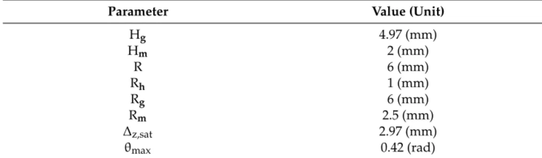
of geometry and material properties. It is feasible to fabricate sensors over reasonable ranges of the height H and the shear modulus G making them appropriate design variables for an optimisation study. Any number of parameters could be selected as design variables for the sensor, including the choice of components not investigated here, but H and G have been chosen to demonstrate how this type of sensor can be optimised by design. The ranges used for each of the design variables were

chosen as H∈ [3, 7]mm and G∈ [1, 5]kPa as to span reasonable values of the identified variables,

the sensor designed by Wang et al. [9] used H = 3 mm and G = 2.94 kPa. The remaining parameters

required for the sensor design and mechanics are given in Table1.

Table 1.Fixed design characteristics of the MagOne sensor.

Parameter Value (Unit)

Hg 4.97 (mm)

Hm 2 (mm)

R 6 (mm)

Rh 1 (mm)

Rg 6 (mm)

Rm 2.5 (mm)

∆z,sat 2.97 (mm)

θmax 0.42 (rad)

2.2.1. Parameterisation

The magnetic fieldBand forceFwere determined over the range of the design variables and

displacements. The responses were subsequently characterised by Equations (14) and (15) as functions

of the parameters G, H, t, andθ. The sensitivityΓwas calculated by taking partial derivatives ofF

with respect toB, leading to Equation (16).

B=f(t,θ, H) (14)

F=f(B, t,θ, G, H) (15)

Γ=f(B, t,θ, G, H) (16)

GP was used to derive phenomenological expressions representing each of Equations (14) and (15), and from which Equation (16) was subsequently determined. The form of these expressions used any mathematical operator with any combination of the input variables. The expressions were derived based on an evolutionary bio-inspired algorithm similar to that used in GAs for optimisation

problems [29], which accurately describe complex non-linear trends in the response that were not

simple (or even possible) to derive from first principles [30]. Due to the non-linearity associated

with the magnetic field and force responses of MagOne under load, GP provided a useful means for

obtaining the algebraic relationships required [20].

2.2.2. Loading Stability

As the sensor is displaced in both the normal and shear directions it is known that the normal

force Fzwill monotonically increase; however, the shear force Frdoes not exhibit the same type of

response and as such the stable region for sensing where an increase in displacement correlates to

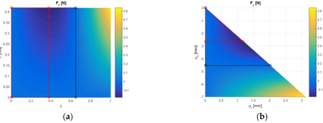
an increase in Fris therefore reduced. The effect of t andθon Fris shown in Figure5a and the effect

of urand uzon Fris shown in Figure5b for when H = 7 mm and G = 5 kPa. The region indicated in

black identifies where Fr is always monotonically decreasing with urfor any given uz, which itself

corresponds to when Fr is negative in value. Further to this, the region identified in red shows the

range of displacements for when Fr is monotonically decreasing from zero to the minimum value

(8)

force and normal force are monotonically changing with displacement and reach peak values at the

same instance.Sensors 2017, 17, 2539 8 of 20

(a) (b)

Figure 5. Response of F in N for H = 7 mm and G = 5 kPa. Region of stable shear loading bounded

in red, point placed at the location the minimum F . Region of negative F bounded in black, point

placed at the location of F = 0 for θ = θ . (a) F shown as a function of t and θ. (b) F shown as

a function of u and u .

With shear loading considered in the design this stability condition was imposed and the bounds

of the feasible displacements reduced to t′ ∈ [0, t ] and θ′ ∈ [0, θ ], where t and θ are the

values of t and θ corresponding to F, for any given value of H and G (see Equation (17)). The

optimisation is performed within these bounds (see Section 2.2.3) but this does not limit the operation of the sensor, only the range of stable displacements which the design is optimised for.

Corresponding to these reduced bounds, the maximum normal force F , and maximum

shear/normal sensitivities Γ, , Γ, can be determined for any given value of H and G by

Equation (18).

: F

: 0 ≤ t ≤ 1, 0 ≤ θ ≤ θ : F, t , θ = f H, G

(17)

: F , Γ , Γ : 0 ≤ t ≤ t , 0 ≤ θ ≤ θ

: F, , Γ, , Γ, = f H, G

(18)

2.2.3. Design Optimisation

The optimisation objective for the sensor design was to minimise the sensitivity Γ over the ranges

of the design variables H and G. In order to achieve this the worst sensitivity (maximum value of Γ)

over all stable displacements was used. The worst sensitivity corresponds to the maximum value of

Γ because this implies the greatest rate of change of F with the measured B. By minimising the worst

sensitivity achieved during displacement ensures that the optimised design has the best possible sensitivity for all displacements considered. By using the stable range of displacements the optimised

sensor was also ensured to produce a monotonically changing F with measured B.

For each case a measureable maximum/minimum force = F, , F, was specified which

subsequently constrained the optimisation such that this force could at least be measured. These force

constraints ensured that the minimum possible shear force the sensor measured F, was less than

or equal to the constrained value F, , and the maximum possible normal force the sensor measured

F , was greater than or equal to the constrained value F , . Given that both force components were

constrained by design, the objective for the optimisation corresponded to minimising the worst

sensitivity in both directions (that is minimising Γ, and Γ, ) as described by the multi-objective

problem, Equation (19). This produced optimal values of the design variables H∗ and G∗ with

corresponding obejctives Γ∗, , Γ∗, and constraints F∗, , F∗, .

Figure 5.Response of Frin N for H = 7 mm and G = 5 kPa. Region of stable shear loading bounded in red, point placed at the location the minimum Fr. Region of negative Frbounded in black, point placed at the location of Fr=0 forθ=θmax. (a) Frshown as a function of t andθ. (b) Frshown as a function of urand uz.

With shear loading considered in the design this stability condition was imposed and the bounds

of the feasible displacements reduced to t0 ∈[0, tm]andθ0∈[0,θm], where tmandθmare the values of

t andθcorresponding to Fr,minfor any given value of H and G (see Equation (17)). The optimisation

is performed within these bounds (see Section2.2.3) but this does not limit the operation of the

sensor, only the range of stable displacements which the design is optimised for. Corresponding to

these reduced bounds, the maximum normal force Fz,maxand maximum shear/normal sensitivities

Γr,max,Γz,maxcan be determined for any given value of H and G by Equation (18).

minimise: Fr

subject to: 0≤t≤1, 0≤θ≤θmax

to yield: Fr,min(tm,θm) =f(H, G)

(17)

maximise: Fz,Γr,Γz

subject to: 0≤t≤tm, 0≤θ≤θm

to yield: Fz,max,Γr,max,Γz,max=f(H, G)

(18)

2.2.3. Design Optimisation

The optimisation objective for the sensor design was to minimise the sensitivityΓover the ranges

of the design variables H and G. In order to achieve this the worst sensitivity (maximum value of

Γ) over all stable displacements was used. The worst sensitivity corresponds to the maximum value

ofΓbecause this implies the greatest rate of change ofFwith the measuredB. By minimising the

worst sensitivity achieved during displacement ensures that the optimised design has the best possible sensitivity for all displacements considered. By using the stable range of displacements the optimised

sensor was also ensured to produce a monotonically changingFwith measuredB.

For each case a measureable maximum/minimum forceFc = (Fr,c, Fz,c)was specified which

subsequently constrained the optimisation such that this force could at least be measured. These force

constraints ensured that the minimum possible shear force the sensor measured Fr,minwas less than

or equal to the constrained value Fr,c, and the maximum possible normal force the sensor measured

Fz,max was greater than or equal to the constrained value Fr,z. Given that both force components

were constrained by design, the objective for the optimisation corresponded to minimising the worst

(9)

problem, Equation (19). This produced optimal values of the design variables H∗ and G∗ with

corresponding obejctivesΓ∗_r,max,Γ∗_z,maxand constraints F∗_r,min, F∗_z,max.

minimise: Γr,maxandΓz,max

subject to: 3≤H≤7[mm], 1≤G≤5[kPa]

Fr,min−Fr,c ≤0, Fc,z−Fz,max≤0

to yield: Γ∗r,max, Γ∗z,max, Fr,min∗ , Fz,max∗ =f(H∗, G∗)

(19)

2.3. Numerical Simulations

2.3.1. Magnetic Field Simulation

In order to calculate the magnetic field components Br, Bz, Equations (9)–(12) were solved and

from whichBwas determined in a fixed cylindrical coordinate system according to the boundary

conditions outlined in Section2.1.2. This was undertaken using the FE method as implemented in the

software COMSOL Multiphysics [31]. The magnetisationMwas chosen based on the characteristics

specified by the manufacturer and the orientation of the magnetic poles. For the sensor concept

developed by Wang et al. [9] Mz=1.2×106A/m and the remaining components were set to zero.

The permeability of free space was given byµ₀=1.257×10−6(m.kg)/(s.A)2.

In the simulation 18,555 second-order triangular elements were used to discretise the domain, with the smallest elements placed on the magnet and grown in size toward the external boundary. This number of elements was shown to be significant in producing grid independent results, with an

increase in accuracy in the measurement ofBof less than 1.34% produced when a greater number of

elements was used. The calculation took approximately 2 min to run on a 2.8 GHz 4-core CPU with

16 GB of RAM. Once the solution was achieved a post-processing stage allowedBto be given as a

function of t,θ, H from the fixed position solution.

2.3.2. Structural Mechanics Simulations

The shear and normal forces Fr, Fz were calculated using a model developed with Abaqus

CAE [32] which employs the FE method. The incompressible Neo-Hookean hyperelastic model was

specified for the material properties, and the boundary conditions implemented were according to

those outlined in Section2.1.3. The magnet and indenting surfaces were represented by rigid bodies

such that they did not deform under load, and the elastomer was rigidly connected to the magnet surfaces such that they had the same displacement. The penalty contact algorithm was used to describe the normal contact pressures due to the interaction of the elastomer and rigid bodies. Tangential

contact tractions were modelled by assigning a coefficient of frictionµ_f=0.45, which is a known value

for rubber-like silicone on a hard surface and represents frictional behaviour similar to that of human

skin [33]. The standard settings for the explicit (time-dependent) solver were used. The time period

for indentation (1 s) was assumed to be large enough for inertia to have no dynamic effect and as such the results produced were quasi-static.

The number of elements used in the structural mechanics simulations varied because the geometry was parameterised by the variable H, therefore a minimum and maximum element size were chosen

to use across all geometries. Minimum and maximum element length scales of 7.5µm and 100µm

were used, respectively, and the resulting discretised domains varied in number from 127,877 to 285,150 second-order tetrahedral elements over the range of H. These values were found to produce

grid-independent results with an increase in accuracy in the measurement ofFof less than 1.88%

found when using smaller element sizes. The meshing procedure ensured that the smallest elements were placed in regions where high stress and strains are produced under load, as such the corner and edge regions on the domain were more densely populated than regions far from boundaries. For each

(10)

indenting surface. The time to compute varied based on the values ofθ, G, H. The longest simulation occurred at the maximum for each parameter and took approximately 3 h 40 min using the same

computer hardware as described in Section2.3.1.

2.3.3. Genetic Programming

The open source toolbox GPTIPS [34] was used to derive phenomenological expressions

representing Equations (14) and (15) by GP. The toolbox is written using the Matlab [35] programming

language. The data required by GPTIPS to calculate these expressions must span the ranges of t,θ, G,

and H; additionally, the corresponding values ofBandFmust be calculated from the simulations as

described in Sections2.3.1and2.3.2. For this purpose a full factorial Design of Experiments (DOE) was

used to select the values of t,θ, G, and H as to ensure that the entire design space was populated in

an evenly-distributed manner. The number of experiments in each dimension were chosen as: 21 in

t; 5 inθ; 5 in H; and 5 in G. The total number of DOE points in theBresponse was 525 which were

obtained from 1 simulation, and the total number of DOE points in theFresponse was 2625, obtained

from 125 simulations (taking approximately 2 weeks to compute using the same computer hardware

as outlined in Section2.3.1).

For each of the expressions generated by GPTIPS the types of mathematical operators which can be used is controlled by the user. The combination of these as functions of the input variables is

chosen to best represent the output data via the use of an evolutionary algorithm [20]. In the case of

deriving equations to represent Equations (14) and (15), the operators were limited to those which can be continuously differentiated so that the derivatives also take analytical forms and can be used in the

optimisation procedure, as outlined in Section2.3.4. The GPTIPS algorithm also allowed control of

parameters relating to the number of genes (or component part of each expression), the complexity of each gene, population size, and solution tolerances. An increase in the number of genes, their complexity, and the population size or decrease in the solver tolerances will increase the likelihood that a more accurate expression is generated; however, this becomes a trade-off with the length of time which the solution takes. In each instance that GPTIPS fits an expression to a data set it is likely that a different solution will be generated. This is because the total number of different combinations of the input and mathematical expressions is very large and by random number generation it is unlikely that the same combinations will be produced. In the case of Equations (14) and (15) the solver

tolerances were reduced to 10−9and the remaining parameters set to their default values. The solver

was subsequently run for 4 h to derive each of the expressions for Br, Bz, Fr, and Fz. These tolerances

and time to compute has been used in previous studies to obtain sufficiently accurate relationships [25].

After calculating these expressions they were differentiated using Matlab to provide the sensitivity

Γr,Γz(Equation (16)) and higher derivatives needed for the optimisation studies.

2.3.4. Optimisation Procedure

The optimisation studies were conducted using the Matlab optimisation toolbox [35]. For each

study the objective formed a minimax type problem with nonlinear constraints [36]. The minimax

condition was satisfied by solving forΓr,maxandΓz,maxas functions of H and G and then subsequently

minimising this value. Similarly, Fr,minand Fz,maxwere determined as functions of H and G for use

in the constraints. Underlying each of these optimisation studies was a sub-optimisation sequence

in whichΓr,max, Γz,max, Fr,minand Fz,maxwere determined as functions of t andθ. Therefore, each

optimisation study was separated into two parts: (i) unconstrained optimisation of sensitivity and force to find the maximum/minimum values for all displacements (Equations (17) and (18)), and (ii) force-constrained optimisation of sensitivity to find the minimum values for all design variables (Equation (19)).

In (i) values of H and G were specified and for whichΓr,max, Γz,max, Fr,minand Fz,maxare to be

determined as functions of t andθ. This was achieved using a GA in combination with a heuristic-based

(11)

heuristic solver; this process ensured that the minimum identified by the GA was refined to the exact

global minimum [21]. Where a maximum was to be found the identity max

x (f(x)) =−minx (−f(x))was

used. The Matlab functiongawas implemented to find the initial guess for the heuristic solver which

was itself the Matlab functionfmincon, for both all tolerances were set to 10−12_{. For}_ga_{the population}

size was set to 200, and withinfminconthe trust-region-reflective-algorithm was chosen to which the

gradients and Hessian ofΓandFwith respect to t andθwere supplied. Due to stability conditions,

Fr,minand the corresponding tmandθmwere solved for first because t0andθ0were required for the

calculation of theΓr,max,Γz,maxand Fz,max.

A GA was used in (ii) to find the minimum values ofΓr,maxand Γz,max returned from (i) as

functions of H and G. This was subject to force constraints for which Fr,min and Fz,max were also

given from (i) as functions of H and G. The Matlab functiongamultiobjwas used in combination with

nonlinear constraints to solve the multi-objective optimisation problem. An equal weighting was applied to the objective function components in order to generate a single cost function which the optimisation algorithm minimises. This subsequently produced a Pareto set of designs which minimise both components without bias. Each part of the Pareto set is equally optimal and a decision making

process was required to establish the optimal design solutionΓr,max∗ , Γ∗z,max, F∗r,min, F∗z,max=f(H∗, G∗).

In each case all tolerances in the solver were specified as 10−12and the population size was set to 200.

For the purpose of this study the force constraints were specified as Fr,c =−0.25 N and Fz,c=5 N,

respectively. The optimisation procedure and corresponding data required for visualisation took approximately 23 h 35 min to compute.

A flow chart outlining the optimisation procedure developed in this work is given in AppendixA

(FigureA1).

2.4. Design Validation

In order to validate the optimised design a set of four new sensors were fabricated according to the

optimised sensor height H∗and material stiffness G∗, as given by the result of the method described in

Section2.3.4. To achieve this a mould was printed using stereolithography at a 25µm resolution [37].

The mould was then cast with a silicone elastomer [38] and left to cure at room temperature. Once

cured, magnets were embedded into the nodes of the sensor bodies with a silicone adhesive [39]. After

ensuring that the magnets were fully encapsulated into the sensor bodies, the sensors were mounted

onto custom designed 3D printed circuit boards for experimental testing [9].

The new sensors (Figure1b) were tested experimentally through a custom test platform consisting

of a force/torque (F/T) sensor [40], mounting brackets, the magnetic sensor and two motorised linear

stages [41] positioned to provide compression in thez-axis and shear force about thex-axis. The linear

stages had a minimum step of 0.01 mm, travel range of 75 mm, and repeatability of 2.5µm, while

the F/T sensor has a measuring range of±35 N in the z-axis,±25 N inx/y–axis, and a resolution of

6.25 mN in all axes. A custom program was developed using LabView [42] to calibrate and control the

movement of the motorised linear stages; this was used to digitally acquire the measurements from the F/T sensor and the magnetic sensor. The step size for the linear stage in all axes was set to the minimum 0.01 mm and the total time taken for each of the indentation tests was ~3 h. This allowed for a high resolution data capture and also assisted in minimising transient and slip effects of the sensor under load. With the aim of ensuring that the observed experimental behaviour is as close as possible to the steady-state assumptions underpinning the simulated response.

Two repeats were made for each indentation test conducted on each of the four newly fabricated sensors, this number was used to ensure that the results obtained were a true representation of the repeatability of the sensor. Results generated from each repeat test were then processed using a

high-band/low-band filter (available from the online Matlab file exchange [43]) in order to reduce

(12)

cut-off bandwidths were specified in the software. Using the filtered data, the mean and standard deviation of the force and magnetic field responses were calculated across all repeats as a function

of the indentation displacement using Equations (20) and (21), respectively. Where N=8 (4 sensors

times 2 repeats) is the total number of indentation tests,ϕare the parameters describing indentation

(displacement for a given shear angle),ψ_iare the response variables (force and magnetic field) for

the I’th repeat test,ψ_µis the mean of the response variables over the number of repeats, andψσis

the standard deviation of the response variables over the number of repeats. In order to assess the

variability in the experimental responses the maximum coefficient of variation cv,ψover the full range

of displacements was calculated using Equation (22). This gives a measure for the variation about

the mean value obtained, with cv,ψapproaching zero implying that the mean is close to all values

obtained over the number of repeats and displacements considered.

ψ_µ(ϕ) = 1

N

i=N

∑

i=1

ψ_i(ϕ) (20)

ψ_σ(ϕ) =

v u u

t1

N

i=N

∑

i=1

(ψ_i(ϕ)−ψµ(ϕ))2 (21)

cv,ψ=max

ϕ

ψ_σ(ϕ)

ψ_µ(ϕ)

×100% (22)

The mean values obtained experimentally were subsequently compared to those generated from GP under the same conditions. This was undertaken by calculating the maximum absolute percentage error between the mean experimental and computational results over the range of displacements,

as described by Equation (23). Whereψare the maximum absolute percentage errors andψare the

response variables obtained computationally from GP. An analysis was then made investigating the sensitivities of the optimised and original designs, in which the percentage difference between the two sets of data obtained from GP for these conditions were calculated and compared.

ψ=max ϕ

ψ_µ(ϕ)−ψ(ϕ)

ψ(ϕ)

×100% (23)

3. Results

3.1. Magnetic Field

Figure 6a,b illustrate Br and Bz distributions, respectively, calculated from the 2D

axially-symmetric FE simulation of the magnetic field as described in Section 2.3.1. Each figure

shows the magnetic field components in the region close to the magnet by means of filled, coloured

contours in units of Tesla. It is demonstrated that the strength of Brand Bzdiminishes with increasing

distance from the magnet in both the r and z directions. Figure6b shows that the distribution of Bzis

symmetric about the centre of the magnet at z = 0 mm, and Figure6a shows that Bris anti-symmetric

about the centre of the magnet where z = 0 mm. The responses generated by GP as a result of the

magnetic field simulation were of a high level of accuracy, with the errors in Brand Bzshown to be

(13)

Sensors2017,17, 2539 13 of 20

the I’th repeat test, is the mean of the response variables over the number of repeats, and is

the standard deviation of the response variables over the number of repeats. In order to assess the

variability in the experimental responses the maximum coefficient of variation c , over the full

range of displacements was calculated using Equation (22). This gives a measure for the variation

about the mean value obtained, with c , approaching zero implying that the mean is close to all

values obtained over the number of repeats and displacements considered.

=1

N (20)

= 1

N − (21)

c , = max × 100% (22)

The mean values obtained experimentally were subsequently compared to those generated from GP under the same conditions. This was undertaken by calculating the maximum absolute percentage error between the mean experimental and computational results over the range of

displacements, as described by Equation (23). Where ϵ are the maximum absolute percentage

errors and are the response variables obtained computationally from GP. An analysis was then made investigating the sensitivities of the optimised and original designs, in which the percentage difference between the two sets of data obtained from GP for these conditions were calculated and compared.

ϵ = max − × 100% (23)

3. Results

3.1. Magnetic Field

Figure 6a,b illustrate B and B distributions, respectively, calculated from the 2D

axially-symmetric FE simulation of the magnetic field as described in Section 2.3.1. Each figure shows the magnetic field components in the region close to the magnet by means of filled, coloured contours in

units of Tesla. It is demonstrated that the strength of B and B diminishes with increasing distance

from the magnet in both the r and z directions. Figure 6b shows that the distribution of B is

symmetric about the centre of the magnet at z = 0 mm, and Figure 6a shows that B is anti-symmetric

about the centre of the magnet where z = 0 mm. The responses generated by GP as a result of the

magnetic field simulation were of a high level of accuracy, with the errors in B and B shown to be

two orders of magnitude smaller than the values obtained from FE.

(a) (b)

Figure 6. Magnetic field distribution in the near magnet region. (a) Coloured by B. (b) Coloured by

B.

Figure 6.Magnetic field distribution in the near magnet region. (a) Coloured by Br. (b) Coloured by Bz.

3.2. Strcutural Mechanics

An example of the structural mechanics results of the MagOne sensor under normal and shear

loading is presented in Figure7, which illustrates the distribution of displacement magnitude in the

elastomer at t = 1,θ= 0.423 rad, H = 7 mm and G = 5 kPa. Due to normal loading the elastomer material

is compressed in the z-direction between the rigid surfaces which due to the boundary conditions

imposed results in±displacement of material in the r-direction. Material is displaced further in the

positive r-direction than the negative because this is the shear loading orientation. It is also shown that under load the elastomer contacts the upper and lower indenting surfaces and since material cannot deform past these locations the shape of the sensor is significantly changed. The responses generated

by GP as a result of the structural mechanics simulations were accurate, with the errors in Frand Fzan

order of magnitude smaller than the values obtained from FE over the full range of t andθ. The shear

force Frobtained from the structural mechanics simulations as a function of the displacements urand

uzis presented in Figure5a and as a function of t andθin Figure5b, corresponding to this the normal

force Fzcalculated monotonically increased with t and remained constant for allθ.

Sensors 2017, 17, 2539 13 of 20

3.2. Strcutural Mechanics

An example of the structural mechanics results of the MagOne sensor under normal and shear loading is presented in Figure 7, which illustrates the distribution of displacement magnitude in the

elastomer at t = 1, θ = 0.423 rad, H = 7 mm and G = 5 kPa. Due to normal loading the elastomer material

is compressed in the z-direction between the rigid surfaces which due to the boundary conditions imposed results in ± displacement of material in the r-direction. Material is displaced further in the positive r-direction than the negative because this is the shear loading orientation. It is also shown that under load the elastomer contacts the upper and lower indenting surfaces and since material cannot deform past these locations the shape of the sensor is significantly changed. The responses generated by GP as a result of the structural mechanics simulations were accurate, with the errors in

F and F an order of magnitude smaller than the values obtained from FE over the full range of t

and θ. The shear force F obtained from the structural mechanics simulations as a function of the

displacements u and u is presented in Figure 5a and as a function of t and θ in Figure 5b,

corresponding to this the normal force F calculated monotonically increased with t and remained

constant for all θ.

Figure 7. Response of displacement magnitude shown in m for the sensor under load at t = 1, θ = 0.423 rad, H = 7 mm and G = 5 kPa.

3.3. Sensitivity

An example of the sensitivity components Γ and Γ produced under load are given in Figure

8a,b, respectively, for H = 7 mm and G = 5 kPa. Each relationship is derived from the force and magnetic field equations generated by GP and are shown as functions of the displacement described

by t and θ. Because the results presented in Sections 3.1 and 3.2 are shown to be accurate it follows

that the sensitivity is also accurately described. Figure 8a,b show that the sensitivity has a non-linear

response as a function of t and θ which can only be described by the solutions obtained

computationally. Figure 8a illustrates that Γ tends to increase with increasing t but the response is

not always monotonic. Γ increases with increasing θ and the response is monotonic. Figure 8b

shows that Γ increases monotonically with both t and θ and is an order of magnitude larger than

Γ.

(a) (b)

Figure 8. Sensitivity responses generated from GP showing the effect of t and θ for H = 7 mm and G

= 5 kPa. (a) Coloured by Γ. (b) Coloured by Γ.

Figure 7.Response of displacement magnitude shown in m for the sensor under load at t = 1,θ= 0.423 rad, H = 7 mm and G = 5 kPa.

3.3. Sensitivity

An example of the sensitivity componentsΓrandΓzproduced under load are given in Figure8a,b,

respectively, for H = 7 mm and G = 5 kPa. Each relationship is derived from the force and magnetic field equations generated by GP and are shown as functions of the displacement described by t

andθ. Because the results presented in Sections 3.1and 3.2are shown to be accurate it follows

that the sensitivity is also accurately described. Figure8a,b show that the sensitivity has a non-linear

response as a function of t andθwhich can only be described by the solutions obtained computationally.

Figure8a illustrates thatΓrtends to increase with increasing t but the response is not always monotonic.

Γr increases with increasingθ and the response is monotonic. Figure8b shows thatΓzincreases

(14)

Sensors2017,17, 2539 14 of 20 3.2. Strcutural Mechanics