Assessing the consistency assumptions underlying network meta-regression using aggregate data

(1)

meta-regression using aggregate data

.

White Rose Research Online URL for this paper:

http://eprints.whiterose.ac.uk/137238/

Version: Published Version

Article:

Donegan, Sarah, Dias, Sofia orcid.org/0000-0002-2172-0221 and Welton, Nicky J. (2018)

Assessing the consistency assumptions underlying network meta-regression using

aggregate data. Research Synthesis Methods. pp. 1-18. ISSN 1759-2887

https://doi.org/10.1002/jrsm.1327

[email protected] https://eprints.whiterose.ac.uk/ Reuse

This article is distributed under the terms of the Creative Commons Attribution (CC BY) licence. This licence allows you to distribute, remix, tweak, and build upon the work, even commercially, as long as you credit the authors for the original work. More information and the full terms of the licence here:

https://creativecommons.org/licenses/

Takedown

If you consider content in White Rose Research Online to be in breach of UK law, please notify us by

(2)

R E S E A R C H A R T I C L E

Assessing the consistency assumptions underlying network

_‐

regression using aggregate data

Sarah Donegan

1

| Sofia Dias

2

| Nicky J. Welton

2

1_{Department of Biostatistics, Waterhouse} Building, University of Liverpool, Liverpool, UK

2_{School of Social and Community} Medicine, University of Bristol, Bristol, UK

Correspondence

Sarah Donegan, Department of Biostatistics, Waterhouse Building, University of Liverpool, Liverpool L69 3GL, UK.

Email: [email protected]

Funding information

Medical Research Council, Grant/Award Number: MR/K021435/1

When numerous treatments exist for a disease (Treatments 1, 2, 3, etc), net-work meta‐_{regression (NMR) examines whether each relative treatment effect} (eg, mean difference for 2 vs 1, 3 vs 1, and 3 vs 2) differs according to a covar-iate (eg, disease severity). Two consistency assumptions underlie NMR: consis-tency of the treatment effects at the covariate value 0 and consisconsis-tency of the regression coefficients for the treatment by covariate interaction. The NMR results may be unreliable when the assumptions do not hold. Furthermore, interactions may exist but are not found because inconsistency of the coeffi-cients is masking them, for example, when the treatment effect increases as the covariate increases using direct evidence but the effect decreases with the increasing covariate using indirect evidence.

We outline existing NMR models that incorporate different types of treatment by covariate interaction. We then introduce models that can be used to assess the consistency assumptions underlying NMR for aggregate data. We extend existing node‐_{splitting models, the unrelated mean effects inconsistency model,} and the design by treatment inconsistency model to incorporate covariate interactions. We propose models for assessing both consistency assumptions simultaneously and models for assessing each of the assumptions in turn to gain a more thorough understanding of consistency.

We apply the methods in a Bayesian framework to trial‐_{level data comparing} antimalarial treatments using the covariate average age and to four fabricated data sets to demonstrate key scenarios.

We discuss the pros and cons of the methods and important considerations when applying models to aggregated data.

K E Y W O R D S

consistency, inconsistency models, network meta‐_{analysis, network meta}‐_{regression, node splitting,}

treatment by covariate interactions

-This is an open access article under the terms of the Creative Commons Attribution License, which permits use, distribution and reproduction in any medium, provided the original work is properly cited.

(3)

1 |

I N T R O D U C T I O N

Reviews often compare multiple treatments for the same condition. In such cases, network meta‐_{analysis (NMA)} can compare all treatments (eg, Treatments 1, 2, and 3)

in a single analysis by estimating the relative treatment effects (eg, log odds ratios) for all treatment pairings (eg, 2 vs 1, 3 vs 1, and 3 vs 2) using direct and indirect evidence.1-3 The key assumption underlying NMA is consistency of the treatments effects across direct and indirect evidence.3 Many methods have been proposed to assess the consistency assumption underlying NMA,4 including node‐_{splitting models}5,6 _{and inconsistency} models, such as the design by treatment (DBT) inconsis-tency model7-11 and the unrelated mean effects (URM) inconsistency model.12

Network meta‐_{regression (NMR) is an extension of} NMA that examines whether a covariate modifies each of the relative treatment effects.13 A covariate may modify each relative treatment effect differently; that is, each treatment comparison may have a different covariate interaction. NMR is used to explore causes

of heterogeneity or inconsistency or when known effect modifiers exist and we wish to present results for different patient groups. Covariates may be characteris-tics of patients (eg, weight), treatments (eg, additional therapy), studies (eg, location), or methods (eg, alloca-tion concealment).14-16

NMR results commonly consist of, for each compari-son, one relative treatment effect estimated at the covariate value 0 (or at the mean covariate value when the NMR model is centered) and one regression coefficient for the treatment by covariate interaction. Consistency assump-tions are required for both of these parameters.17-19 For instance, for a three‐_{treatment NMR, where Treatment 1} is taken as the reference, the consistency equation for the relative treatment effects can be written as,d23=d13−d12

where, for example,d23is the relative treatment effect for 3

vs 2, and the consistency equation for the regression coef-ficients isβ23 =β13− β12 where, for example,β23is the

[image:3.595.86.512.353.570.2]

coefficient for 3 vs 2.13,17,19 It is possible for neither assumption to hold (ie, inconsistent relative treatment effects and inconsistent coefficients) or for only one of the assumptions to hold (ie, either consistent relative

(4)

treatment effects or consistent coefficients), which would make the results of the NMR unreliable.

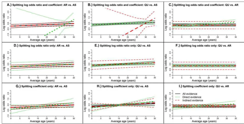
Theoretically, there are eight possible scenarios that can occur when assessing whether treatment by covariate interactions exist and the consistency assumptions. Examples of the scenarios are shown in Figure 1A‐_H. Each figure shows how the relative treatment effect for 3 vs 2 changes with an increasing covariate value; sepa-rate lines are displayed for direct, indirect, and all evi-dence. For a three‐_{treatment network, the direct} evidence for 3 vs 2 would be from trials that allocated Treatments 2 and 3 and the indirect evidence for 3 vs 2 would be from the remaining trials. Note that the lines have the same intercept when the relative treatment effects at the covariate value 0 are consistent (Figure 1 A‐_{D) and the lines have the same slope when the} coeffi-cients are consistent (Figure 1A, B, E, and F). In Figure 1A, no interaction is detected using NMR, and both consistency assumptions are satisfied; therefore, the NMR results are valid but would not be clinically use-ful. On the other hand, in Figure 1B, NMR shows an interaction and both assumptions hold; therefore, the NMR is reliable and could be used to draw clinical infer-ences. Figure 1C, E, and G show scenarios where no interaction is detected using NMR, but one or more of the assumptions are not satisfied; consequently, the NMR results are invalid; notably, in Figure 1C,G, an interaction exists when direct evidence, and indirect evi-dence are considered separately, but it is not seen when applying NMR because it is masked by the inconsistency. Lastly, in Figure 1D, F, and H, an interaction is found using NMR, but one or more of the assumptions do not hold, so the NMR results are unreliable. The cause of inconsistency should be considered when inconsistency is found (Figures 1C‐_H).

Although many methodological publications have proposed NMR analyses,13,17-25 to the authors' knowl-edge, no methods have been introduced for assessing the consistency assumptions underlying NMR.

In this paper, we introduce methods for assessing the consistency assumptions underlying NMR. We extend existing node‐_{splitting models,}5,6 _{the DBT inconsistency} model,7-11 and the URM inconsistency model12to incor-porate treatment by covariate interactions. In Section 2, we specify the NMR model and propose assessment methods that can be applied to aggregate trial‐_{level data} (ie, trial specific relative treatment effects relative to refer-ence Arm 1 and their variances) with either continuous or categorical covariates. In Section 3, we apply the methods to a real data set and fabricated data sets illus-trating key scenarios under a Bayesian framework. In Section 4, we discuss the proposed methods and highlight their pros and cons.

2 |

M E T H O D S

We outline NMR models and then introduce methods for assessing consistency using the node‐_{splitting models and} one type of inconsistency model (ie, URM model). New methods based on the alternative DBT inconsistency model are also presented in the supplementary material. All models are summarized in Table 1.

To set notation, letidenote the trial wherei= 1,…_,S

andSis the number of independent trials and letkbe the trial arm wherek= 1,…_,A_iandA_iis the number of arms in triali. Let tik denote the treatment given in triali in armkwheretik∈{1,……,T} andTis the number of treat-ments in the network. Note that Treatment 1 is taken to be the reference treatment.

Suppose we have trial‐_{level outcome data, where}_y_ik_is the observed relative treatment effect (eg, log odds ratio or mean difference) for armk vs Arm 1 (with k ≥2) in triali andvikis the corresponding variance. As the rela-tive treatment effect is a continuous measure, we assume a normal likelihood y_ik~N(θik,vik) where θik is the mean relative treatment effect in triali (withk≥ 2). Also, the data set would include a study‐_{level covariate} xifor each trial i that can be a continuous variable or an indicator variable to represent dichotomous data.

2.1 |

Network meta

‐

regression models

NMR models estimate the basic regression coefficients, which are the coefficients for each treatment vs Treat-ment 1 (ie,β12,β13,…,β1T), and then the remaining func-tional coefficients (ie,β23,β24,….) are calculated as linear

combinations of the basic coefficients using the consis-tency equations. Three NMR models have been proposed previously, each making different assumptions regarding the basic coefficients,13,17-19 that is, independent (model 1a), exchangeable (model 1b), and common coefficients (model 1c). The decision regarding which assumption to make can be based on model fit statistics and the esti-mated coefficients of the models but in practice is often determined by data availability.

Model 1a can be written as follows:

θik¼δi;1kþβti1;tikxi;

Where β_t_i₁;tik=β1;tik‐β1;ti1,βti1;tik is the difference in the

relative treatment effect of tik vs ti1per unit increase in

(5)

[image:5.595.143.743.157.446.2]

TABLE 1 Proposed model variations

Models Including Independent Treatment by Covariate Interactions

Models Including Exchangeable Treatment by Covariate Interactions

Models Including Common Treatment by Covariate Interactions

NMR Models Model 1a Model 1b Model 1c

Node‐splitting models Models splitting the relative treatment effect and

the regression coefficient for the interaction.

Model 2.1a Model 2.1b Model 2.1c

Models splitting the relative treatment effect only. Model 2.2a Model 2.2b Model 2.2c

Models splitting the regression coefficient for the interaction only.

URM models Models assessing consistency of the relative

treatment effect and the regression coefficient for the interaction.

Models assessing consistency of the relative treatment effect only.

Models assessing consistency of the regression coefficient for the interaction only.

DBT models Models assessing consistency of the relative

treatment effect and the regression coefficient for the interaction.

Models assessing consistency of the relative treatment effect only.

Models assessing consistency of the regression coefficient for the interaction only.

Abbreviations: DBT, design by treatment; NMR, network meta‐regression; URM, unrelated mean effects.

DONEGA

N

ET

AL

(6)

realization from a normal distribution δi;1k∼N dti1;tik;σ 2

withdti1;tik ¼d1;tik−d1;ti1wheredti1;tik is the mean relative

treatment effect oftikvsti1when the covariate is 0. In a

fixed‐_{effect model, we set} _σ2 _{= 0 to obtain} _δ_i_,1_k₌ d1;tik −d1;ti1.

Model 1b is the same as model 1a, but now, β₁_;_t_ik

∼Norm Bð ;υ2Þ: Model 1c is formulated by setting β1;tik

¼βin model 1a; note that in this model, the functional coefficients are 0 because of the consistency equations (eg,β23=β13−β12=β−β= 0).17

2.2 |

Assessing consistency by node

splitting

The principle aim of node‐_{splitting models is to assess} whether there is evidence of“_{loop inconsistency,}”_where loop inconsistency is defined as a difference between a result from direct and indirect evidence. Node‐_splitting models estimate relative treatment effects and/or regres-sion coefficients for the interaction based on direct evi-dence and separate estimates from indirect evievi-dence to explore whether they agree. Multiple node‐_splitting models need to be applied, one model for each compari-son of interest.

To specify the node‐_{splitting models, we extend the} notation, such that the node being split is (bt,t*) where bt≠t*and bt<t*:For example, if one wants to split the

node (3,4), thenbt ¼3 andt*= 4.

To assess both the consistency assumptions simulta-neously, node‐_{splitting models can split the relative} treatment effect and coefficient to provide, for each comparison with both direct and indirect evidence, a rel-ative treatment effect, and a coefficient estimated from direct evidence and an effect and coefficient based on indirect evidence. The model that splits the relative treat-ment effect and coefficient and includes independent interactions (model 2.1a) is an extension of model 1a as follows:

θik¼

δi;1kþβti1;tikxi if ti1≠bt and=or tik≠t

*

δi;1kþβdirxi if ti1¼bt and tik¼t*

:; 8

< :

Whereβ_t_i₁_;_t_ik=β₁_;_t_ik‐_β

1;ti1,βti1;tikrepresents the difference

in the relative treatment effect of t_ik vs t_i₁ per unit increase in the covariate estimated using indirect evi-dence, and βdir represents the difference in the relative treatment effect oft*vsbtper unit increase in the covariate estimated using direct evidence. In a random‐_effects model, if trialiallocatedt*andbt, that is,ti1=btandtik=t*, then δi,1k~N(ddir,σ2) where ddir represents the mean

relative treatment effect of t*vs bt when the covariate value is 0 estimated using direct evidence; whereas if trial

idid not allocatet*andbt, that is,ti1≠btand/ortik≠t*, then

δi;1k∼N dti1;tik;σ

2_where _d

ti1;tik represents the mean

rela-tive treatment effect oftikvsti1when the covariate value

is 0 estimated using indirect evidence and dti1;tik

¼d1;tik−d1;ti1.

To assess only the consistency of the relative treat-ment effects, node‐_{splitting models can split the relative} treatment effect alone to produce a single coefficient that is estimated using all evidence and two relative treatment effects (ie, one estimated using direct evidence and the other estimated using the indirect evidence). The model that splits the relative treatment effect alone and includes independent interactions (model 2.2a) is

θik¼δi;1kþβti1;tikxi;

whereβ_t_i₁_;_t_ik represents the difference in the relative treat-ment effect oft_ikvs.t_i₁per unit increase in the covariate estimated using all evidence. In this model, the trial‐ specific relative treatment effects, δi,1kare distributed in the same way as in model 2.1a.

Likewise, to assess the consistency of the coefficients alone, a node‐_{splitting model can split only the coefficient} to estimate a single relative treatment effect using all evi-dence and two coefficients (e, one estimated from direct evidence and the other from indirect evidence). The model that splits only the coefficient and includes inde-pendent interactions (model 2.3a) is the same as model 2.1a except the trial‐_{specific relative treatment effects;}

δi,1k are distributed as δi;1k∼N dti1;tik;σ

2_where _d

ti1;tik

represents the mean relative treatment effect of tik vs ti1

when the covariate value is 0 estimated using all evidence. Node‐_{splitting models can be adapted to include} exchangeable (models 2.1b, 2.2b, and 2.3b) or common (models 2.1c, 2.2c, and 2.3c) interactions as described in Section 2.1. Note that model 2.1c and 2.3c fix each func-tional coefficient based on indirect evidence (ie, β_t_i₁_;_t_ik

when ti1≠ 1) to be 0 whereas the corresponding result

from direct evidence (βdir) is not.

(7)

with that estimated using indirect evidence. Such com-parisons are subjective and when results are presented graphically and compared, care must be taken because the scale and shape of the plots can affect how different the results appear to be. Furthermore, when using Bayes-ian methods, for each comparison, the probability (prob) that the direct and indirect evidence differs can be calcu-lated. For each treatment pairing, the inconsistency esti-mate (IE); that is, the difference between the relative treatment effect from direct evidence and indirect evi-dence can be calculated at each iteration of the chain, and the number of iterations for whichIE≥0 is counted. It is then possible to calculate the prob that the relative treatment effect from direct evidence exceeds the relative treatment effect from indirect evidence, by dividing the number of counted iterations by the total number of iter-ations of the chain. Lastly, assuming that the posterior distribution of the difference (IE) is symmetric and unimodal, the prob that the direct and indirect evidence agree is given by P = 2 × minimum(prob, 1 − prob).5,26

Likewise, the regression coefficients from direct and indi-rect evidence can be compared in the same way.

2.3 |

Assessing consistency using URM

models

URM models assess global consistency that is inconsis-tency somewhere in the treatment network, by compar-ing the results from an NMR model with those from an URM model.12

The URM model that assesses the consistency of the relative treatment effects and coefficients and includes independent interactions (model 3.1a) is the same as the NMR model (model 1a), but it does not incorporate the consistency equations (i.e. dti1;tik ¼d1;tik−d1;ti1 and

β_t_i₁;tik=β1;tik‐β1;ti1), and as such, the model parameters are estimated using direct evidence only. Model 3.1a is equiv-alent to fitting separate pair‐_{wise meta}‐_regressions, except, model 3.1a assumes the between trial variance (σ2) is equal across comparisons but the pair‐_{wise meta}‐ regressions would not.

The URM model that assesses only consistency of the relative treatment effects and includes independent inter-actions (model 3.2a) is the same as model 3.1a but incor-porates the consistency equation for the coefficients. Likewise, the UMR model that assesses only consistency of the coefficients with independent interactions (model 3.3a) is same as model 3.1a but includes the consistency equation for the relative treatment effects.

Exchangeable (models 3.1b, 3.2b, and 3.3b) or com-mon (models 3.1c, 3.2c, and 3.3c) interactions can be included. However, it is worth noting that the

independent, exchangeable, or common assumptions are slightly different to those specified for the NMR models (models 1a, 1b, and 1c). In the NMR models, we assume the basic regression coefficients (ie,β12, β13, …,β1T) are independent, exchangeable, or common. However, when the consistency equation for the coefficients is not used in the URM model (ie, models 3.1[a, b, or c] and 3.3[a, b, or c) we can assume that all regression coefficients, that is basic and functional coefficients, are independent, exchangeable (ie, β_t_i₁_;_t_ik∼Norm B_ð ;υ2_Þ_{) or common (ie,}

β_t_i₁_;_t_ik ¼βÞ. In particular, this means that when including common interactions, the functional coefficients in the NMR model (model 1c) are forced to be 0, but this is not so in the URM model (models 3.1c and 3.3c).

To determine consistency, the model fit of the NMR model (model 1[a, b, or c]) and the fit of the URM models (models 3.1(a, b, or c), 3.2(a, b, or c), and 3.3[(a, b, or c]) can be compared; when an URM model is an improved fit, inconsistency may be present. Also, differences between the relative treatment effects and regression coefficients produced from the NMR model and those from the URM models may suggest inconsistency.

2.4 |

Including multi

‐

arm trials

The models can be applied to data sets including multi‐ arm trials providing that the correlation between the observed relative treatment effect (yik) and the trial‐ specific relative treatment effects (δi,1k) is taken into account. For each multi‐_{arm trial} _i _with _m _{arms, the} observed relative treatment effects and the trial‐_specific relative treatment effects are assumed to follow multivar-iate normal distributions

yi2 ⋮ yim 0 B @ 1 C AeN θi2 ⋮ θim 0 B @ 1 C A;

vi2 … cov yð i2;yimÞ

⋮ ⋱ ⋮

cov yð i2;yimÞ … vim

0 B @ 1 C A 0 B @ 1 C A and

δi;12

⋮

δi;1m 0 B @ 1 C AeN

d1;ti2−d1;ti1 ⋮

d1;tim−d1;ti1 0 B @ 1 C A;

τ2 … _τ2₌₂

⋮ ⋱ ⋮

τ2=2 … _τ2

0 B @ 1 C A 0 B @ 1 C A:

Furthermore, there is an extra consideration when fitting node‐_{splitting models.}5,6_{If one wants to split node} (ti1,tik), then a multi‐arm trial will contribute direct evi-dence to the relative treatment effect (ddir) as required becausebt¼ti1. However, the multi‐arm trial would not

contribute direct evidence to the estimation of the relative treatment effect,ddir, if one splits another node (eg, ti2,

(8)

when a multi‐_{arm trial compared the two treatments,}_t* andbt, in addition to other treatments, treatmentbtis taken to be the baseline treatmentti1for that study.

Note that for URM models including multi‐_{arm trial} data, the URM model is not the same as fitting separate pair‐_{wise meta}‐_{regressions because the correlation in} multi‐_{arm trials is taken into account but would not be} in pair‐_{wise analyses; also, the URM model only uses}_t_i₁ as the baseline treatment so direct evidence for some pairwise comparisons would not be used whereas pairwise meta‐_{regression could utilize all direct evidence.}

3 |

A P P L I C A T I O N T O D A T A S E T S

3.1 |

Data sets

Here, the methods proposed in Section 2 are applied to a real data set and four fabricated data sets that have been manipulated to demonstrate specific scenarios.

3.1.1 |

Malaria data set

Two Cochrane reviews and the corresponding trials were used to construct the malaria data set; reviews compared artemether (AR), quinine (QU), and artesunate (AS).27,28 Randomised controlled trials including patients with severe malaria were eligible. Age was considered to be an effect modifier because the clinical features of malaria differ by age and thus, all treatment recommendations are stratified by age in the reviews and World Health Organization treatment guidelines.29 Event rates for the primary outcome, death, and the covariate, average age of patients in each trial were extracted. Two studies with missing covariate data were deleted from the data set. Using the event rates, trial‐_{specific log odds ratios and} their standard deviations were calculated in R. Table S1 displays the data. Figure 2 shows the network diagram.

3.1.2 |

Fabricated data sets

Four fabricated data sets were constructed by manipulat-ing the malaria data set to illustrate key scenarios: (a) no interaction is present and the relative treatment effects and regression coefficients are consistent (Figure 1A); (b) interaction exists and the relative treatment effects and coefficients are consistent (Figure 1B); (c) interaction exists, and the relative treatment effects are consistent, but the coefficients are inconsistent (Figure 1D); (4) no interaction is present, and the relative treatment effects are consistent, but the coefficients are inconsistent (Figure 1G). Example R code to generate the data sets is given in the supplementary material.

Analogous to the malaria data set, each data set com-pared three treatments (AS, AR, QU): there was direct evidence for each possible comparison; no multi‐_arm tri-als contributed; and a dichotomous outcome and contin-uous covariate was of interest. Ten trials contributed direct evidence to each comparison. For each study, a continuous covariate was taken to be a realization from normal distribution (ie, N(17, 102)) truncated at 0 to ensure the covariate values were similar to those observed in the malaria data set.

The log odds ratios and regression coefficients were chosen to be similar to those estimated in the original data set. For each data set, the log odd ratio at 0 covariate of tri-als comparing treatments AR and AS was 0.2, tritri-als com-paring treatments QU and AS was 0.23, and trials of treatments QU and AR was 0.03. For data set one, the coef-ficient for each comparison was 0. For data set two, the coefficient for trials comparing treatments AR and AS was 0.02, trials comparing treatments QU and AS was 0.02, and trials of treatments QU and AR was 0. For data set three, the coefficient for trials comparing treatments AR and AS was 0.01, trials of treatments QU and AS was 0.04, and trials comparing treatments QU and AR was 0. For data set four, the coefficient for trials comparing treat-ments AR and AS was−0.04, trials of treatments QU and

AS was 0.04, and trials of treatments QU and AR was 0. The trial‐_{specific observed log odds ratios were} esti-mated from the values of log odds ratio at 0 covariate, the coefficients, and the covariates. The between‐_trial var-iance was 0. The standard error of the observed log odds ratio was 0.2 for each trial.

3.2 |

Implementation

[image:8.595.63.270.553.688.2]

All models were fitted to the data sets using WinBUGS 1.4.3 and the R2WinBUGS package in R. Example code is provided as supplementary material. For the malaria data set, all models in Table 1 were fitted. For the fabricated

(9)

data sets, only fixed‐_{effect versions of models 1a}_,_{2.1a, 3.1a,} and 4.1a were applied because the between trial variance was 0 and the coefficients differed across comparisons. See Table S2 for the parameterization of the DBT models. The covariates were centered at their mean. All parameters were given noninformative normal prior distributions (ie,

N(0, 100000)) except the between‐_{trial standard deviation} that was assumed to follow a noninformative uniform dis-tribution (ie,Uni(0, 10)) and a weakly informative prior distribution (ie,uniform(0, 2)) was specified for the stan-dard deviation of the exchangeable regression coefficients. Three chains with different initial values were run for 300 000 iterations. The initial 100 000 draws were discarded and chains were thinned such that every fifth iteration was retained. Convergence of the chains was assessed by inspecting trace plots of the draws.

Model fit and complexity of models was assessed using the deviance information criterion (DIC) defined as

DIC¼Dþp_DwhereDis the posterior mean of the resid-ual deviance andpD is the effective number of parame-ters.30 A model with a smaller DIC was preferable to a model with a larger DIC, but differences of less than three units were not considered meaningful. When models had little difference in DIC, the simplest model was chosen.

3.3 |

Results

Results from NMR, node‐_{splitting and URM models are} presented here. The results from DBT models are pre-sented in supplementary material.

3.3.1 |

Malaria data set

NMR models

Comparing fixed‐_{effect and random}‐_{effect NMR models} (models 1a, 1b, 1c), the DICs from all NMR models vari-ations are similar (DICs 24.93‐_{26.76 in Table S3). Also,} the estimated regression coefficients for the treatment by average age interactions were quite similar for each model variation (Table S4). Therefore, results from the simplest model to the fixed‐_{effect NMR with common} interactions (model 1c) are presented.

The results of model 1c show that there is evidence of a small interaction between relative treatment effect and average age for AR vs AS and QU vs AS; the posterior median of the common regression coefficient for AR vs AS and QU vs. AS is 0.0132 with 95% credibility interval (CrI), 0.0018‐_{0.0244, (Table S4). There is no interaction} for QU vs AR because the model fixes the coefficient to be 0. However, before using these results to draw clinical inferences, the underlying consistency assumptions must be assessed.

Node‐splitting models

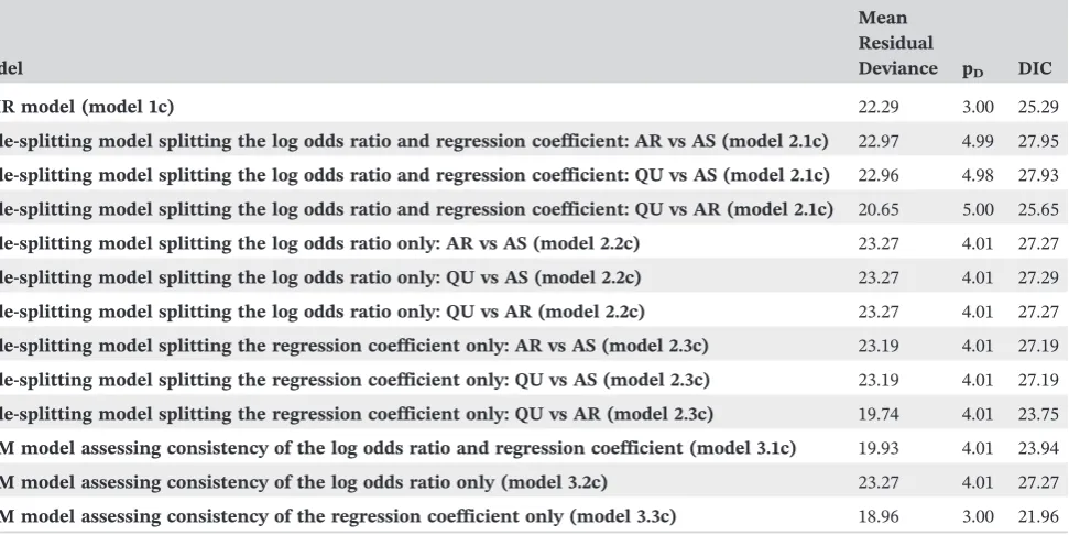
[image:9.595.65.551.465.708.2]

Table 2 shows model fit assessment results for fixed‐_effect node‐_{splitting models with common interactions (models} 2.1c, 2.2c, 2.3c). The DIC of the NMR model (DIC = 25.29) is similar to those of the node‐_{splitting models (DICs} 23.75‐_{27.95) indicating that the model is not improved} by splitting each node, lending support to the consistency assumptions.

TABLE 2 Model fit assessment results for fixed‐_{effect models with common treatment by average age interactions for the malaria data set}

Model

Mean Residual

Deviance pD DIC

NMR model (model 1c) 22.29 3.00 25.29

Node‐splitting model splitting the log odds ratio and regression coefficient: AR vs AS (model 2.1c) 22.97 4.99 27.95

Node‐splitting model splitting the log odds ratio and regression coefficient: QU vs AS (model 2.1c) 22.96 4.98 27.93

Node‐splitting model splitting the log odds ratio and regression coefficient: QU vs AR (model 2.1c) 20.65 5.00 25.65

Node‐splitting model splitting the log odds ratio only: AR vs AS (model 2.2c) 23.27 4.01 27.27

Node‐splitting model splitting the log odds ratio only: QU vs AS (model 2.2c) 23.27 4.01 27.29

Node‐splitting model splitting the log odds ratio only: QU vs AR (model 2.2c) 23.27 4.01 27.27

Node‐splitting model splitting the regression coefficient only: AR vs AS (model 2.3c) 23.19 4.01 27.19

Node‐splitting model splitting the regression coefficient only: QU vs AS (model 2.3c) 23.19 4.01 27.19

Node‐splitting model splitting the regression coefficient only: QU vs AR (model 2.3c) 19.74 4.01 23.75

URM model assessing consistency of the log odds ratio and regression coefficient (model 3.1c) 19.93 4.01 23.94

URM model assessing consistency of the log odds ratio only (model 3.2c) 23.27 4.01 27.27

URM model assessing consistency of the regression coefficient only (model 3.3c) 18.96 3.00 21.96

Abbreviations: AR, artemether; AS, artesunate; DIC, deviance information criterion; QU, quinine; NMR, network meta‐_{regression; URM, unrelated mean}

(10)

[image:10.595.50.739.157.424.2]

TABLE 3 Results from fixed‐_{effect node}‐_{splitting models including common treatment by average age interactions for the malaria data set}

Model Type Parameter Evidence

Posterior Median (95% Credibility Interval),P

AR vs AS QU vs AS QU vs AR

Splitting the log odds ratio and regression coefficient (model 2.1c)

Log odds ratio (centered) Direct −2.3540 (−6.7650 to 2.0530)* 0.4316 (0.2833‐0.5797) 0.2882 (0.0449‐0.5315)

Indirect 0.1985 (−0.0815 to 0.4782) −2.1000 (−6.4180 to 2.4430)* 0.1825 (−0.4751 to 0.8419)

IE,P −2.5510 (−6.9740 to 1.8710), P= 0.26

2.5330 (−2.0150 to 6.8540), P= 0.26

0.1055 (−0.5990 to 0.8089), P= 0.77

Regression coefficient for the interaction

Direct 0.1738 (−0.0974 to 0.4451) 0.0126 (0.0006‐0.0245) 0.0191 (−0.0008 to 0.0387)

Indirect 0.0126 (0.0007‐_0.0245) _{0.1728 (}

−0.1048 to 0.4376) Fixed at 0 IE,P 0.1613 (−0.1100 to 0.4327),

P= 0.25

−0.1603 (−0.4253 to 0.1173), P= 0.24

0.0191 (−0.0008 to 0.0387), P= 0.06

Splitting the log odds ratio only (model 2.2c)

Log odds ratio (centered) Direct 0.2495 (−0.3804 to 0.8815) 0.4320 (0.2837‐0.5804) 0.2328 (−0.0031 to 0.4700)

Indirect 0.1994 (−0.0821 to 0.4787) 0.4824 (−0.1946 to 1.1600) 0.1816 (−0.4797 to 0.8403)

IE,P 0.0512 (−0.6481 to 0.7515), P= 0.89

−0.0499 (−0.7523 to 0.6552), P= 0.89

0.0521 (−0.6518 to 0.7545), P= 0.89

All 0.0129 (0.0011‐_0.0248) _{0.0129 (0.0011}‐_0.0248) _{Fixed at 0}

Splitting the regression coefficient only (model 2.3c)

Log odds ratio (centered) All 0.1890 (−0.0918 to 0.4673) 0.4283 (0.2793‐0.5747) 0.2746 (0.0469‐0.5033)

Direct 0.0195 (−0.0210 to 0.0603) 0.0126 (0.0007‐0.0245) 0.0188 (−0.0007 to 0.0385)

Indirect 0.0125 (0.0007‐_0.0245) _{0.0194 (}

−0.0210 to 0.0601) Fixed at 0 IE,P 0.0070 (−0.0358 to 0.0500),

P= 0.75

−0.0068 (−0.0498 to 0.0357), P= 0.76

0.0188 (−0.0007 to 0.0385), P= 0.06

Abbreviations: AR, artemether; AS, artesunate; IE, inconsistency estimate;P, probability of agreement between direct and indirect evidence; QU, quinine. * Results are influenced by the vague prior distribution and can be considered to be“_{not estimable.}”

N

ET

AL

.

(11)

[image:11.595.85.512.185.379.2]

The results from node splitting are displayed in Table 3. In the model that assesses consistency of both the log odds ratio and the coefficient (model 2.1c), the log odds ratios for AR vs AS (−2.3540, 95% CrI,−6.7650

to 2.0530) and QU vs AS (0.4316, 95% CrI, 0.2833‐ 0.5797) based on direct evidence differs with those from indirect evidence (ie, 0.1985, 95% CrI,−0.0815 to 0.4782,

and −2.1000, 95% CrI, −6.4180 to 2.4430, respectively)

because only two trials contribute direct evidence for

[image:11.595.84.509.460.676.2]

AR vs.AS and, therefore, the results are influenced by the vague prior distribution. A similar but less pro-nounced inconsistency is also seen for the corresponding coefficients. Yet the prob of agreement between direct and indirect evidence is low for the coefficient for QU vs AR (P = 0.06) but not remarkably low for other com-parisons or the log odds ratios (Ps 0.24‐_{0.77). Similar} con-clusions are drawn from models that split either the log odds ratio or the regression coefficient only (models 2.2c

FIGURE 3 Posterior distributions for the log odds ratios (centered) and regression coefficients for the interaction from fixed‐_{effect node}‐ splitting models with common treatment by average age interactions for the malaria data set. Results in Figure A‐_{F are from models 2.1c and} 1c. Results in Figures G‐_{I are from models 2.2c and 1c. Results in Figures J}‐_{L are from models 2.3c and 1c. In Figures F and I, the coefficient} from indirect evidence and from all evidence is forced to be 0. AR, artemether; AS, artesunate; QU, quinine

(12)

and 2.3c). The consistency of the direct and indirect evi-dence is also supported graphically in Figure 3, which displays the posterior distributions of the centered log odds ratios and regression coefficients and in Figure 4, where the log odds ratio versus average age is plotted.

URM models

Table 2 also displays model fit assessment results for fixed‐_{effect URM models with common interactions} (models 3.1c, 3.2c, 3.3c). The DIC of the NMR model (DIC = 25.29) is similar to those from the URM models the assess consistency of both the log odds ratio and coef-ficient (DIC = 23.94) or the log odds ratio alone (DIC = 27.27) (models 3.1c and 3.2c) but is slightly higher than that from the model that assesses the coefficient alone (DIC = 21.96) (model 3.3c) indicating a possible inconsistency on a coefficient.

See Table 4 for the results from the NMR model and URM models. The results from the URM models are quite similar to those from the NMR model with the exception of the regression coefficient for QU vs AR. This difference in the coefficient for QU vs AR is because of the different assumptions underlying the two models; the NMR model sets the regression coefficients for AR vs AS and QU vs AS to be identical (ie, 0.0132, 95% CrI, 0.0018‐_0.0244) and the coefficient for QU vs AR to be 0, whereas all three coefficients are set to be identical in the URM model (ie, 0.0145, 95% CrI, 0.0044‐_0.0247).

Overall, there is not only evidence of an interaction from the NMR but also evidence of inconsistency; the node‐_{splitting models show evidence of loop} inconsis-tency for the coefficient of QU vs AR, and the URM models support this showing a possible inconsistency of the coefficients.

3.3.2 |

Fabricated data sets

Data set 1: No interaction and consistency

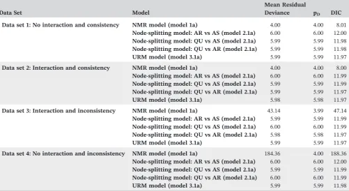
[image:12.595.319.537.56.732.2]

The DICs from each model (models 1a, 2.1a, and 3.1a) are similar (8.01‐_{12.00); therefore, there is no obvious sign of} inconsistency (Table 5). Using the results from node split-ting (model 2.1a), the log odds ratios and coefficients based on direct and indirect evidence are very similar, and the probabilities of agreement between direct and indirect evidence are practically one (Table 6). The results from the NMR model are also similar to those from the URM model (model 3.1a) (Table 7) indicating consis-tency. Overall, the NMR model does not show that a treatment by average age interaction exists (Table 7) and there is no evidence of loop inconsistency using node splitting or global inconsistency using the URM model. Figure 5, which shows the results from the NMR model and node‐_{splitting models, supports this conclusion.} TABLE

(13)

Data set 2: Interaction and consistency

The DICs from the models (models 1a, 2.1a, and 3.1a) are again similar (8.00‐_{11.99) indicating consistent evidence} (Table 5). From node splitting (model 2.1a), the log odds ratios and the coefficients based on direct and indirect evidence are almost identical, and the probabilities of agreement of direct and indirect evidence are practically one (Table 6); Figure 5 shows the results graphically. The URM model (model 3.1a) also gives comparable results to the NMR model (Table 7). In conclusion, the NMR model shows that an interaction exists for AR vs AS (0.0200, 95% CrI, 0.0074‐_{0.0327) and QU vs AS} (0.0200, 95% CrI, 0.0080‐_{0.0321) (Table 7) and there is} no loop inconsistency using node splitting, or global inconsistency using the URM model.

Data set 3: Interaction and inconsistency

The DIC from the NMR model (model 1a) (DIC = 47.14) is much higher than those from node splitting (model 2.1a) and the URM model (model 3.1a) (11.97‐_11.99) sug-gesting inconsistency (Table 5). From node splitting, the log odds ratios based on direct and indirect evidence are comparable, but the coefficients for AR vs AS (0.0100, 95% CrI,−0.0039 to 0.0241) and QU vs AS (0.0400, 95%

CrI, 0.0298 to 0.0503) and QU vs AR (0.0000, 95% CrI,

−0.0125 to 0.0126) from direct evidence differ from those

from indirect evidence (ie, 0.0400, 95% CrI, 0.0237‐_0.0562, 0.0099, 95% CrI,−0.0088 to 0.0289, and 0.0300, 95% CrI,

0.0127‐_{0.0474, respectively); the probabilities of} agree-ment of direct and indirect evidence are very high (Ps 0.9982‐_{0.9990) for the log odds ratios and very low for} the coefficients (Ps 0.0057‐_{0.0062) (Table 6). The URM} model also gives results that differ somewhat from those of the NMR model (see Table 7). To summarise, the NMR model shows that an interaction exists for AR vs AS (0.0187, 95% CrI, 0.0082‐_{0.0292), QU vs AS (0.0335,} 95% CrI, 0.0244‐_{0.0425), and QU vs AR (0.0147, 95%} CrI, 0.0047‐_{0.0248) (Table 7) but there is also loop} incon-sistency in the size of the underlying coefficients based on direct and indirect evidence that is seen using node split-ting (Figure 5); the URM model identifies global inconsistency.

Data set 4: No interaction and inconsistency

The DIC from the NMR model (model 1a) (DIC = 188.36) is much higher than those from node splitting (model 2.1a) and the URM model (model 3.1a) (11.99‐_12.00) indi-cating inconsistency (Table 5). Similar to data set 3, in node‐_{splitting models, the log odds ratios based on direct} and indirect evidence are comparable, but the coefficients for AR vs. AS (−0.0400, 95% CrI,−0.0553 to−0.0246) and

[image:13.595.48.550.74.348.2]

QU vs. AS (0.0400, 95% CrI, 0.0273‐_{0.0529) and QU vs AR}

TABLE 5 Model fit assessment results for fixed‐_{effect models assessing consistency of both the log odds ratio and regression coefficient} with independent treatment by average age interactions for the fabricated data sets

Data Set Model

Mean Residual

Deviance pD DIC

Data set 1: No interaction and consistency NMR model (model 1a) 4.00 4.00 8.01

Node‐splitting model: AR vs AS (model 2.1a) 6.00 6.00 12.00

Node‐splitting model: QU vs AS (model 2.1a) 5.99 5.99 11.98

Node‐splitting model: QU vs AR (model 2.1a) 5.99 5.99 11.98

URM model (model 3.1a) 5.99 5.99 11.97

Data set 2: Interaction and consistency NMR model (model 1a) 4.00 4.00 8.00

URM model (model 3.1a) 5.98 5.98 11.97

Data set 3: Interaction and inconsistency NMR model (model 1a) 43.14 3.99 47.14

URM model (model 3.1a) 5.99 5.99 11.97

Data set 4: No interaction and inconsistency NMR model (model 1a) 184.36 4.00 188.36

URM model (model 3.1a) 5.99 5.99 11.98

Abbreviations: AR, artemether; AS, artesunate; DIC, deviance information criterion; QU, quinine; NMR, network meta‐_{regression; URM, unrelated mean}

(14)

[image:14.595.53.746.98.512.2]

TABLE 6 Results from fixed‐_{effect node}‐_{splitting models splitting both the log odds ratio and regression coefficient including independent treatment by average age interactions (model 2.1a)}

for the fabricated data sets

Data Set Parameter Evidence

Posterior Median (95% Credibility Interval),P

Log odds ratio (uncentered) Direct 0.1997 (−0.0948 to 0.4949) 0.2302 (−0.0566 to 0.5139) 0.0298 (−0.2356 to 0.2937)

Indirect 0.2001 (−0.1865 to 0.5902) 0.2306 (−0.1642 to 0.6265) 0.0297 (−0.3799 to 0.4398)

IE,P −0.0007 (−0.4870 to 0.4894), P= 0.9974

−0.0004 (−0.4879 to 0.4875), P= 0.9986

−0.0002 (−0.4891 to 0.4886), P= 0.9990

Direct 0.0000 (−0.0107 to 0.0109) 0.0000 (−0.0135 to 0.0136) 0.0000 (−0.0115 to 0.0116)

Indirect 0.0000 (−0.0178 to 0.0178) 0.0000 (−0.0158 to 0.0158) 0.0000 (−0.0174 to 0.0174)

IE,P 0.0000 (−0.0210 to 0.0208), P= 0.9980

0.0000 (−0.0208 to 0.0209), P= 0.9980

0.0000 (−0.0208 to 0.0209), P= 0.9982

Log odds ratio (uncentered) Direct 0.1992 (−0.1284 to 0.5285) 0.2300 (−0.0268 to 0.4852) 0.0301 (−0.3372 to 0.3941)

Indirect 0.1998 (−0.2432 to 0.6460) 0.2304 (−0.2614 to 0.7213) 0.0299 (−0.3886 to 0.4447)

IE,P −0.0007 (−0.5528 to 0.5534), P= 0.9980

−0.0001 (−0.5549 to 0.5537), P= 0.9998

−0.0003 (−0.5542 to 0.5548), P= 0.9996

Direct 0.0200 (0.0049‐_0.0352) _{0.0200 (0.0069}‐_0.0333) _{0.0000 (}₋_{0.0239 to 0.0240)}

Indirect 0.0200 (−0.0073 to 0.0473) 0.0199 (−0.0084 to 0.0485) 0.0000 (−0.0200 to 0.0201)

IE,P 0.0000 (−0.0313 to 0.0312), P= 0.9974

0.0001 (−0.0315 to 0.0313), P= 0.9954

0.0000 (−0.0311 to 0.0313), P= 1.0000

Log odds ratio (uncentered) Direct 0.2000 (−0.1389, 0.5372) 0.2301 (−0.0208, 0.4796) 0.0301 (−0.2355 to 0.2937)

Indirect 0.1999 (−0.1619, 0.5649) 0.2304 (−0.1985, 0.6584) 0.0299 (−0.3924 to 0.4492)

IE,P 0.0003 (−0.4955 to 0.4950), P= 0.9990

−0.0006 (−0.4948 to 0.4955), P= 0.9982

−0.0004 (−0.4971 to 0.4983), P= 0.9986

Direct 0.0100 (−0.0039 to 0.0241) 0.0400 (0.0298‐0.0503) 0.0000 (−0.0125, 0.0126)

Indirect 0.0400 (0.0237‐_0.0562) _{0.0099 (}₋_{0.0088 to 0.0289)} _{0.0300 (0.0127}‐_0.0474)

IE,P −0.0300 (−0.0515 to−0.0088), P= 0.0059

0.0301 (0.0085‐_0.0514),

P= 0.0062

−0.0300 (−0.0515 to−0.0086), P= 0.0057

Data set 4: No interaction and

inconsistency

Log odds ratio (uncentered) Direct 0.2002 (−0.0926 to 0.4908) 0.2300 (0.0222‐0.4360) 0.0297 (−0.2260 to 0.2863)

Indirect 0.2000 (−0.1290, 0.5298) 0.2300 (−0.1569, 0.6178) 0.0301 (−0.3279 to 0.3866)

IE,P −0.0003 (−0.4376 to 0.4397), P= 0.9990

−0.0007 (−0.4393 to 0.4399), P= 0.9976

0.0000 (−0.4398 to 0.4398), P= 1.0000

Direct −0.0400 (−0.0553 to−0.0246) 0.0400 (0.0273 to 0.0529) 0.0000 (−0.0115 to 0.0116)

Indirect 0.0399 (0.0227, 0.0574) −0.0400 (−0.0591,−0.0208) 0.0800 (0.0600‐0.1000)

IE,P −0.0799 (−0.1031 to−0.0571), P= 0.0000

0.0800 (0.0568‐_0.1030),

P= 0.0000

−0.0800 (−0.1031 to−0.0569), P= 0.0000

Abbreviations: AR, artemether; AS, artesunate; IE, inconsistency estimate;P, probability of agreement between direct and indirect evidence; QU, quinine. Posterior median (95% credibility interval) presented.

N

ET

AL

.

(15)

[image:15.595.60.744.143.471.2]

TABLE 7 Results from fixed‐_{effect network meta}‐_{regression and unrelated mean effects models assessing consistency of both the log odds ratio and regression coefficient with independent}

treatment by average age interactions for the fabricated data sets

Data Set Model Parameter

Posterior Median (95% Credibility Interval)

NMR model (model 1a) Log odds ratio (uncentered) 0.2002 (−0.0305 to 0.4281) 0.2302 (0.0014‐0.4587) 0.0306 (−0.1911 to 0.2517)

0.0000 (−0.0090 to 0.0091) 0.0000 (−0.0102 to 0.0102) 0.0000 (−0.0096 to 0.0096)

URM model (model 3.1a) Log odds ratio (uncentered) 0.2002 (−0.0947 to 0.4926) 0.2301 (−0.0556 to 0.5148) 0.0303 (−0.2340 to 0.2937)

0.0000 (−0.0108 to 0.0108) 0.0000 (−0.0135 to 0.0136) 0.0000 (−0.0116 to 0.0116)

NMR model (model 1a) Log odds ratio (uncentered) 0.2006 (−0.0539 to 0.4514) 0.2302 (0.0043‐0.4558) 0.0298 (−0.2223 to 0.2828)

0.0200 (0.0074‐_0.0327) _{0.0200 (0.0080}‐_0.0321) _{0.0000 (}

−0.0147 to 0.0147)

0.0200 (0.0049‐_0.0351) _{0.0200 (0.0068}‐_0.0332) _{0.0000 (}₋_{0.0240 to 0.0240)}

NMR model (model 1a) Log odds ratio (uncentered) 0.2081 (−0.0390 to 0.4523) 0.1654 (−0.0503 to 0.3808) −0.0421 (−0.2636 to 0.1801)

0.0187 (0.0082‐0.0292) 0.0335 (0.0244‐0.0425) 0.0147 (0.0047‐0.0248)

0.0100 (−0.0040 to 0.0240) 0.0400 (0.0297‐0.0503) 0.0000 (−0.0125 to 0.0125)

Data set 4: No interaction and inconsistency

NMR model (model 1a) Log odds ratio (uncentered) 0.0877 (−0.1296 to 0.3034) 0.3389 (0.1566‐0.5214) 0.2515 (0.0472‐0.4567)

−0.0098 (−0.0211 to 0.0017) −0.0001 (−0.0105 to 0.0103) 0.0097 (−0.0002 to 0.0195)

URM model (model 3.1a) Log odds ratio (uncentered) 0.2004 (−0.0911 to 0.4899) 0.2302 (0.0231‐0.4372) 0.0305 (−0.2259 to 0.2854)

−0.0400 (−0.0553 to−0.0247) 0.0400 (0.0272‐0.0529) 0.0000 (−0.0115 to 0.0116)

Abbreviation: AR, artemether; AS, artesunate; NMR, network meta‐regression; QU, quinine; URM, unrelated mean effects.

DONEGA

N

ET

AL

(16)

(0.0000, 95% CrI, −0.0115 to 0.0116) from direct

evi-dence differ from those from indirect evievi-dence (ie, 0.0399, 95% CrI, 0.0227‐_0.0574, ₋_{0.0400, 95% CrI,}

−0.0591 to −0.0208, and 0.0800, 95% CrI, 0.0600‐

0.1000, respectively); the probabilities of agreement of direct and indirect evidence are very high for log odds ratios (Ps 0.9976‐_{1.000) and 0 for the coefficients} (Table 6). Also, results from the URM model are differ-ent from those of the NMR model (see Table 7). Over-all, the NMR model shows that no interaction exists (Table 7) but there is inconsistency in the direction of the underlying coefficients based on direct and indirect evidence and this trend can be seen using node split-ting (Figure 5); the URM model suggests global incon-sistency respectively, but these models cannot show the underlying trend.

4 |

D I S C U S S I O N

[image:16.595.85.510.45.444.2]

We have shown that node‐_{splitting and inconsistency} models can be useful for assessing the underlying consis-tency assumptions of NMR when using aggregate data. Once consistency has been assessed, the analyst must decide which results to present. If the direct and indirect evidence are consistent, the results from the NMR should be reliable. However, the level of heterogeneity (from the NMR or standard pairwise analyses) and goodness of fit of the NMR should be considered when drawing conclu-sions from the results. If there is inconsistency, the results from the NMR are questionable and the causes of incon-sistency should be considered. In some scenarios, for example, when inconsistency masks an interaction, as shown in Figure 1C,G, the results would not be useable.

(17)

If the original purpose of the NMR was to explore causes of heterogeneity or inconsistency in an NMA and there is no interaction and no inconsistency masking interactions in the NMR, then analysts could proceed by exploring other potentially relative treatment effect modifying covariates or reconsidering the eligibility criteria.

Each of the proposed methods has different pros and cons. DBT models assess design and loop consistency and can assess global inconsistency, while node splitting assesses loop consistency and URM models assess global inconsistency; loop inconsistency is well recognized in the methodological literature but design consistency is a newer concept.7,11Furthermore, the DBT model requires parameterization by the analyst; therefore, the analyst needs to have a good understanding of the model and parameters. Key advantages of the DBT model and node splitting is that IEs and the prob that direct and indirect evidence agree can be obtained; however, the URM model does not provide such results. Moreover, concerns regarding multiple testing may apply to node‐_splitting and the DBT models where probabilities are calculated, particularly when a Frequentist approach is taken; there-fore, it is important to compare model fit statistics across models, and also to be cautious in interpreting“_P_values” making sure to allow for multiple testing. One disadvan-tage of node splitting is that, as one model is fitted for every comparison with contributing direct and indirect evidence, many models may need to be fitted, which is computationally demanding, whereas only one inconsis-tency model would need to be applied.

Ideally, all three approaches (ie, node‐_{splitting model,} DBT model, and URM model) would be applied to pro-vide a thorough assessment of consistency. However, in practice, the reviewer may select their preferred approach depending on the ease of application in software etc. We recommend that at least one of the global tests (ie, incon-sistency models) and also node splitting are performed. Our preference is node splitting because estimates from direct and indirect evidence can be found.

We proposed and applied methods to trial‐_level aggregated data in this article. However, it is straightfor-ward to adapt the models to accommodate any type of arm‐_{level outcome data, that is, a summary of the} out-come data for each arm of each trial and a covariate value for each trial. To adapt the models, a suitable link function would be chosen and nuisance parameters are included in the model to represent the effect of the base-line treatment in Arm 1 of triali. Further details regard-ing arm‐_{level NMA models are given by Dias, Sutton,} Ades, and Welton31

Moreover, collection and use of individual patient data is generally advantageous over aggregate data when studying patient‐_{level covariates because they avoid}

ecological biases.32,33 Yet it is more common to explore patient‐_{level covariates (eg, patient age) using study}‐_level covariate summaries (eg, average age of patients) in meta‐ regression such as in the malaria data set. However, when using aggregate data, the possibility of confounding and ecological biases should be considered when patient‐ level covariates are explored.

There are a number of issues that can arise when applying the methods, particularly with aggregate data. Parameter estimation can be a problem with limited data, such that models cannot be fitted at all, interactions exist but cannot be detected, or inconsistency exists but is not found. For instance, when all the trials that contribute to the estimation of a regression coefficient have the same covariate value or when only one trial contributes to a coefficient, this would preclude the use of models with independent interactions, but analysts may be able to apply a model with exchangeable or common interactions providing studies that contribute to another basic coeffi-cient that has different covariate values. For example, when exploring an interaction between relative treatment effect and study location (ie, continent), studies that con-tribute to results for Comparison 2 vs 1 may all be carried out on the same continent provided that studies that tribute to Comparison 3 vs 1 are located on different con-tinents. Parameter estimation may particularly be a problem when fitting the DBT model because the IEs would be imprecise when the number of trials in one or more designs is limited; to overcome this one could assume exchangeability of the inconsistency factors or use informative prior distributions. Similarly, if direct evi-dence is limited for some comparisons (ie, few trials or covariate values), the URM model and node‐_splitting models would produce imprecise results, and informative prior distributions may need to be used. Ideally, any informative prior distributions would be evidence based by eliciting them from similar meta‐_{analyses or experts'} beliefs. Finally, it is also worth emphasising that no evi-dence of inconsistency does not automatically imply there is consistency; inconsistency may exist but cannot be detected when data are limited and results are imprecise, and therefore, arguably the consistency assumptions and the NMR results are questionable. In the same way, in such cases, no evidence of a treatment by covariate inter-action does not imply there is truly no interinter-action.

(18)

In conclusion, consistency of the assumptions under-lying NMR must be assessed when NMR is applied, even when no treatment by covariate interactions are detected. It is possible that inconsistency is masking an interaction. Furthermore, results of an NMR should not be reported without assessing the underlying assumptions to deter-mine whether the results are valid and reliable.

A C K N O W L E D G E M E N T S

This research was funded by the Medical Research Coun-cil (http://www.mrc.ac.uk/, grant number MR/K021435/ 1) as part of a career development award in biostatistics awarded to SDo. We are grateful to the two anonymous peer reviewers for their helpful comments.

C O N F L I C T O F I N T E R E S T

The authors have declared no competing interests exist.

A U T H O R C O N T R I B U T I O N S

SDo proposed extending the existing node‐_splitting models proposed by SDi and NW and inconsistency models to include treatment by covariate interactions. NW proposed additional modelling extensions. SDo car-ried out the analysis and wrote the first draft of the man-uscript. SDi and NW provided statistical guidance and commented on the manuscript.

O R C I D

Sarah Donegan http://orcid.org/0000-0003-1709-2290

Sofia Dias http://orcid.org/0000-0002-2172-0221

R E F E R E N C E S

1. Higgins J, Whitehead A. Borrowing strength from external trials in a meta‐_analysis._{Stat Med}_{. 1996;15(24):2733}‐_2749.

2. Lu G, Ades A. Combination of direct and indirect evidence in mixed treatment comparisons.Stat Med. 2004;23(20):3105‐_3124. 3. Lu G, Ades A. Assessing evidence inconsistency in mixed

treat-ment comparisons.J Am Stat Assoc. 2006;101(474):447‐_459. 4. Donegan S, Williamson P, D'alessandro U, Tudur Smith C.

Assessing key assumptions of network meta‐_{analysis: a review} of methods.Res Syn Meth. 2013a;4(4):291‐_323.

5. Dias S, Welton NJ, Caldwell DM, Ades AE. Checking consis-tency in mixed treatment comparison meta‐_analysis._{Stat Med}_. 2010;29(7‐_8):932‐_944.

6. Van Valkenhoef G, Dias S, Ades AE, Welton NJ. Automated generation of node‐_{splitting models for assessment of} inconsis-tency in network meta‐_analysis._{Res Syn Meth}_{. 2016;7(1):80}‐_93.

7. Higgins JPT, Jackson D, Barrett JK, Lu G, Ades AE, White IR. Consistency and inconsistency in network meta‐_analysis: con-cepts and models for multi‐_{arm studies.} _{Res Syn Meth}_. 2012;3(2):98‐110.

8. Jackson D, Barrett JK, Rice S, White IR, Higgins JPT. A design‐ by‐_{treatment interaction model for network meta}‐_{analysis with} random inconsistency effects.Stat Med. 2014;33(21):3639‐_3654. 9. Jackson D, Boddington P, White IR. The design‐by‐treatment

interaction model: a unifying framework for modelling loop inconsistency in network meta‐_analysis. _Res _Syn _Meth_. 2016;7(3):329‐_332.

10. Law M, Jackson D, Turner R, Rhodes K, Viechtbauer W. Two new methods to fit models for network meta‐_{analysis with}

ran-dom inconsistency effects. BMC Med Res Methodol.

2016;16(1):87.

11. White IR, Barrett JK, Jackson D, Higgins JPT. Consistency and inconsistency in network meta‐_{analysis: model estimation using} multivariate meta‐_regression._{Res Syn Meth}_{. 2012;3(2):111}‐_125. 12. Dias S, Welton NJ, Sutton AJ, Caldwell DM, Lu G, Ades AE.

Evidence synthesis for decision making 4: inconsistency in net-works of evidence based on randomized controlled trials.Med Decis Making. 2013c;33(5):641‐_656.

13. Dias S, Sutton AJ, Welton NJ, Ades AE. Evidence synthesis for decision making 3: heterogeneity—subgroups, meta‐regression, bias, and bias‐_adjustment. _{Med Decis Making}_{. 2013b;33(5):} 618‐_640.

14. Thompson S, Sharp S. Explaining heterogeneity in meta‐ analysis: a comparison of methods. Stat Med. 1999;18(20): 2693‐_2708.

15. Thompson SG. Systematic review: why sources of heterogeneity in meta‐_{analysis should be investigated.}_BMJ_{. 1994;309(6965):} 1351‐1355.

16. Thompson SG, Higgins JPT. How should meta‐_regression analyses be undertaken and interpreted?Stat Med. 2002;21(11): 1559‐_1573.

17. Cooper N, Sutton A, Morris D, Ades A, Welton N. Addressing between‐_{study heterogeneity and inconsistency in mixed} treat-ment comparisons: application to stroke prevention treattreat-ments in individuals with non‐_{rheumatic atrial fibrillation.}_{Stat Med}_. 2009;28(14):1861‐1881.

18. Donegan S, Williamson P, D'alessandro U, Garner P, Tudur Smith C. Combining individual patient data and aggregate data in mixed treatment comparison meta‐_{analysis: individual} patient data may be beneficial if only for a subset of trials.Stat Med. 2013b;32(6):914‐_930.

19. Donegan S, Williamson P, D'alessandro U, Tudur Smith C. Assessing the consistency assumption by exploring treatment by covariate interactions in mixed treatment comparison meta‐ analysis: individual patient‐_{level covariates versus aggregate} trial‐_{level covariates.}_{Stat Med}_{. 2012;31(29):3840}‐_3857.

20. Jansen J, Cope S. Meta‐_{regression models to address} heterogene-ity and inconsistency in network meta‐analysis of survival outcomes.BMC Med Res Methodol. 2012;12(1):152.

(19)

22. Nixon RM, Bansback N, Brennan A. Using mixed treatment comparisons and meta‐_{regression to perform indirect} compari-sons to estimate the efficacy of biologic treatments in rheumatoid arthritis.Stat Med. 2007;26(6):1237‐1254.

23. Salanti G, Marinho V, Higgins JPT. A case study of multiple‐ treatments meta‐analysis demonstrates that covariates should be considered.J Clin Epidemiol. 2009;62(8):857‐_864.

24. Saramago P, Sutton AJ, Cooper NJ, Manca A. Mixed treatment comparisons using aggregate and individual participant level data.Stat Med. 2012;31(28):3516‐_3536.

25. Tudur Smith C, Marson A, Chadwick D, Williamson P. Multiple treatment comparisons in epilepsy monotherapy trials. Trials. 2007;8(1):34.

26. Marshall E, Spiegelhalter D. Identifying outliers in Bayesian hierarchical models: a simulation‐_{based approach.} _Bayesian

Anal. 2007;2(2):409‐444.

27. Esu E, Effa EE, Opie ON, Uwaoma A, Meremikwu MM. Artemether for severe malaria. Cochrane Database Syst Rev. 2014;9:CD010678.

28. Sinclair D, Donegan S, Isba R, Lalloo David G. Artesunate ver-sus quinine for treating severe malaria. Cochrane Database Syst Rev. 2012;6:CD005967.

29. World Health Organisation 2015.Guidelines for the treatment of malaria. Third edition ed.

30. Spiegelhalter DJ, Best NG, Carlin BP, Van Der Linde A. Bayes-ian measures of model complexity and fit.Med Decis Making. 2002;64:583‐_639.

31. Dias S, Sutton AJ, Ades AE, Welton NJ. Evidence synthesis for decision making 2: a generalized linear modeling framework for pairwise and network meta‐_{analysis of randomized} con-trolled trials.Med Decis Making. 2013a;33(5):607‐617.

32. Riley RD, Lambert PC, Staessen JA, et al. Meta‐_{analysis of} con-tinuous outcomes combining individual patient data and aggregate data.Stat Med. 2008;27(11):1870‐_1893.

33. Riley RD, Steyerberg EW. Meta‐analysis of a binary outcome using individual participant data and aggregate data. Res Syn Meth. 2010;1(1):2‐_19.

34. Lu G, Ades A. Modeling between‐_{trial variance structure in} mixed treatment comparisons.Biostatistics. 2009;10(4):792‐_805.

S U P P O R T I N G I N F O R M A T I O N

Additional supporting information may be found online in the Supporting Information section at the end of the article.

How to cite this article: Donegan S, Dias S, Welton NJ. Assessing the consistency assumptions underlying network meta‐_{regression using}