Adaptive multivariate global testing

Full Terms & Conditions of access and use can be found at

http://www.tandfonline.com/action/journalInformation?journalCode=uasa20

Journal of the American Statistical Association

ISSN: 0162-1459 (Print) 1537-274X (Online) Journal homepage: http://www.tandfonline.com/loi/uasa20

Adaptive Multivariate Global Testing

Giorgos Minas, John A.D. Aston & Nigel Stallard

To cite this article: Giorgos Minas, John A.D. Aston & Nigel Stallard (2014) Adaptive Multivariate Global Testing, Journal of the American Statistical Association, 109:506, 613-623, DOI:

10.1080/01621459.2013.870905

To link to this article: https://doi.org/10.1080/01621459.2013.870905

Published with License by Taylor & Francis© Giorgos Minas, John Aston, Nigel Stallard

View supplementary material

Accepted author version posted online: 19 Dec 2013.

Published online: 19 Dec 2013. Submit your article to this journal

Article views: 1443

View Crossmark data

Adaptive Multivariate Global Testing

Giorgos M

, John A.D. A

, and Nigel S

We present a methodology for dealing with recent challenges in testing global hypotheses using multivariate observations. The proposed tests target situations, often arising in emerging applications of neuroimaging, where the sample sizenis relatively small compared with the observations’ dimensionK. We employ adaptive designs allowing for sequential modifications of the test statistics adapting to accumulated data. The adaptations are optimal in the sense of maximizing the predictive power of the test at each interim analysis while still controlling the Type I error. Optimality is obtained by a general result applicable to typical adaptive design settings. Further, we prove that the potentially high-dimensional design space of the tests can be reduced to a low-dimensional projection space enabling us to perform simpler power analysis studies, including comparisons to alternative tests. We illustrate the substantial improvement in efficiency that the proposed tests can make over standard tests, especially in the case ofnsmaller or slightly larger thanK. The methods are also studied empirically using both simulated data and data from an EEG study, where the use of prior knowledge substantially increases the power of the test. Supplementary materials for this article are available online.

KEY WORDS: Adaptive design; Multivariate test; Neuroimaging; Power analysis.

1. INTRODUCTION

In this work, we develop novel methodology for dealing with recent challenges in testing global hypotheses using multivari-ate observations. The classical approach for studying the prob-lem, Hotelling’sT2-test (Hotelling1931), can efficiently detect effects in every direction of the multivariate space when the sample sizenis sufficiently large. However, in settings wheren

approaches or becomes smaller than the observation dimension

K,T2_{-test becomes respectively inefficient and inapplicable.} This cost in efficiency, paid due to the need to search in every direction of the alternative space, seems particularly wasteful (but avoidable), if prior knowledge about the direction of the effect is available. Motivated by the latter settings, often arising in the increasingly important field of neuroimaging, we develop tests which are powerful in studies withnK, but can also be efficient in situations wherenis close to or smaller thanK.

The proposed tests employ adaptive designs allowing for se-quential modifications of the test statistic based on accumulated data. Such adaptive designs have straightforward but not ex-clusive application in clinical trials. A large literature on the subject (e.g., Bauer and K¨ohne1994; Proschan and Hunsberger

1995; Lehmacher and Wassmer1999; M¨uller and Sch¨afer2001; Brannath, Posch, and Bauer2002; Liu, Proschan, and Pledger

2002; Brannath, Gutjahr, and Bauer2012) deals with the deriva-tion of flexible procedures that allow for adaptaderiva-tions of the initial design without inflation of the Type I error rate. Some sequen-tial designs (e.g., Denne and Jennison2000) also permit design adaptations, but the latter need to be preplanned and indepen-dent of the interim test statistics. Adaptive designs are employed

©Giorgos Minas, John Aston, Nigel Stallard. This is an Open Access ar-ticle distributed under the terms of the Creative Commons Attribution License (http://creativecommons.org/licenses/by/3.0/), which permits unrestricted use, distribution, and reproduction in any medium, provided the original work is properly cited. The moral rights of the named author(s) have been asserted.

Giorgos Minas (E-mail: [email protected]) and John A. D. Aston (E-mail:[email protected]), Department of Statistics, Uni-versity of Warwick, Coventry, CV4 7AL, UK. Nigel Stallard, Division of Health Sciences, Warwick Medical School, University of Warwick, UK (E-mail: [email protected]). The authors would like to express their thanks to an AE and two referees for comments which helped improve the article. J.A.D.A. acknowledges partial support for this work from EPSRC Grant EP/K021672/1. Color versions of one or more of the figures in the article can be found online atwww.tandfonline.com/r/jasa.

for many kinds of adaptations including sample size recalcula-tion (Lehmacher and Wassmer1999; Mehta and Pocock2011), treatment or hypothesis selection (Kimani, Stallard, and Hutton

2009), and sample allocation to treatments (Zhu and Hu2010). Despite the fact that many authors have stressed the potential for test statistic adaptation (e.g., Bauer and K¨ohne1994; Bretz et al.2009), there are only a few papers on the subject (Lang, Auterith, and Bauer2000; Kieser, Schneider, and Friede2002). Furthermore, various approaches for adaptive designs in multi-ple testing are available (see Bretz et al.2009). These methods can efficiently detect few independently significant outcomes. However, it is well known that standard multiple testing meth-ods (e.g., Bonferroni and Simes tests) become conservative and inefficient in settings, such as the typical neuroimaging studies, where strong dependencies and a large number of outcomes are present (D’Agostino and Russell2005).

Similarly to the tests developed by O’Brien (1984), L¨auter, Glimm, and Kropf (1998), and Minas et al. (2012), the proposed tests are based on linear combinations of the observation vec-tors. The crucial element in this approach is the weighting vector reducing the observation vectors to the scalar linear combina-tions. This defines the direction in which we decide to search for effects, and it can substantially affect both Type I and Type II error rate of the tests. O’Brien proposed deriving the weight-ing vectors under the assumption of uniform mean structure, while L¨auter et al. showed that if the weighting vector is derived from the observation sums of products matrix, the Type I error is controlled and high power is attained under certain factorial structures. On the other hand, the tests in Minas et al. (2012) can attain high power levels independently of the mean and co-variance structure but a part of the sample is used in a separate pilot study to learn the weighting vector.

In this work, linear combination test statistics, initially con-structed using weighting vectors derived from prior information, are sequentially updated based on observed data at subsequent interim analyses in an adaptive design. Early termination of the study (due to early acceptance or rejection of the null hypothesis

Published with License by Taylor & Francis Journal of the American Statistical Association June 2014, Vol. 109, No. 506, Theory and Methods

DOI:10.1080/01621459.2013.870905

at an interim analyses) which is often of interest, especially in clinical trials, is also possible within our approach. Our meth-ods provide a formal framework for optimally using prior in-formation in constructing test statistics as has been suggested, but not implemented, in earlier papers (Pocock, Geller, and Tsiatis1987; L¨auter, Glimm, and Kropf1996; Tang, Gnecco, and Geller1989a).

While our tests maintain the two prime targets of adaptive de-signs, namely flexibility and Type I error control (Brannath et al.

2012), we also focus on attaining power optimality. Specifically, we employ the methods proposed by Spiegelhalter, Abrams, and Myles (2002) to derive optimal tests maximizing the predictive power of the test at each interim analysis. The methods of proofs can be useful in deriving optimal adaptive designs in more gen-eral settings. As we illustrate in Section3, the results of Theorem 3.1 could be used to derive optimal designs for regression anal-ysis for example.

The power performance of a multivariate test, lying in a pos-sibly high-dimensional design space, can be hard to illustrate and interpret. Therefore, power analysis of multivariate tests is typically restricted to a limited part of the design space. We tackle this problem by reexpressing theO(K2)-dimensional de-sign space as a lower dimensional easily interpretable space that is still sufficient to determine power. The crucial step here is to identify a measure quantifying the angular distance between the selected weighting vector and the optimal weighting vector and proving its sufficiency in computing power. These results pro-vide wide understanding of the behavior of linear combination tests and allow us to extend earlier work on power analysis of single stage (Pocock, Geller, and Tsiatis1987; Follmann1996; Logan and Tamhane2004) and sequential (Tang, Gnecco, and Geller 1989b; Tang, Geller, and Pocock 1993) linear combi-nation tests, beyond low-dimensional observations or specific mean and covariance structures.

We perform extensive simulation studies to explore and com-pare the proposed and alternative single stage and sequential procedures throughout the design space. We show that linear combination tests outperform Hotelling’sT2-tests for the latter angular distance being below a certain value which, especially for sample sizes close toK, can be rather high. We further show that, in contrast to linear combination tests, such as O’Brien OLS test, with fixed weighting vectors, the adaptive linear com-bination tests can attain high power levels even in situations where the weighting vector selected at the planning stage is or-thogonal to the true optimal (where, of course, a nonadaptive test would have zero power asymptotically). The advantages of the proposed tests are also illustrated through a real example taken from an EEG depression study (L¨auter, Glimm, and Kropf

1996).

This article is organized as follows. In Section 2, we for-mulate the class of linear combination tests while in Section 3 we derive optimal, with respect to power, tests in this class. In Section4, we present the results allowing us to characterize power based on low-dimensional summaries of the design pa-rameters. In Section5, we discuss the main results of extensive simulation studies performed using the latter results to explore power and compare the proposed tests with alternative global tests under various conditions, while in Section6we apply our procedures to an EEG depression study. Section 7 includes a

short summary and discussion of the obtained results. Technical lemmas and proofs are provided in Supplementary Material A, while further illustrations of the simulation studies are provided in Supplementary Material B.

2. FORMULATION OFJ-STAGE LINEAR COMBINATION TESTS

In the following, we formulateJ-stage linear combinationz andt-tests and define their error rate functions. We assume that theK-dimensional observation vectorsY_ij =(Y_ij1, . . . , YijK)T of subjects i=1,2, . . . , n_j, participating in stage j, j = 1,2, . . . , J, of the study, are independent and identically dis-tributed Gaussian random variables

Yij ∼NK(μ,), (2.1)

with meanμ=(μ1, . . . , μK)T and covariance matrix the

posi-tive definite=(σ_kk)K_k,k=1. In medical applications, the mean vector is often interpreted as the treatment effect. We wish to test the global null hypothesis of no treatment effectH0:μ= 0=(0,0, . . . ,0)Tagainst the two-sided alternativeH1 :μ=0. Note that the methods which follow equally apply to the two-sample test with common covariance matrix, but we continue with the one-sample presentation to simplify notation.

The observation vectors Yij, i=1,2, . . . , nj, of the jth stage are projected on the nonzero weighting vector w_j = (w_j1, wj2, . . . , wjK)T and the projection magnitudes form the linear combinations L_ij =wT_jY_ij,i=1,2, . . . , n_j, j = 1,2, . . . , J. The stagewise z and t statistics for testing H0 against H1 using the random sample of linear combinations

Lij,i=1, . . . , nj, when is either known or unknown, are

respectively

Zj =

¯

Lj σj/n1j/2

, Tj =

¯

Lj sj/n1j/2

. (2.2)

Here,σ2

j is the variance and ¯Lj,sj2 are the sample mean and

sample variance of the linear combinationL_j, respectively. Un-der assumption (2.1), the stagewise zandt statistics,Z_j,T_j,

j =1,2, . . . , J are respectively normally and noncentrally t

distributed, Z_j ∼N( ¯θ_j,1) andT_j ∼t_νj( ¯θ_j) with location pa-rameter

¯

θj =θj√nj, θj = w T jμ

wT

jwj1/2

, (2.3)

and νj =nj−1. Under H0, the z and t statistics are stan-dard normal and Student’s t random variables, that is, Zj ∼ N(0,1) and Tj ∼tνj. The two-sided stagewise p values of thezandt-tests are, respectively,p_zj =2(−|Zj|) andp_tj = 2_νj(−|T_j|),where(·) and(·) are the cumulative distribu-tion funcdistribu-tions of the standard normal and Student’st-distribution withν_j degrees of freedom, respectively.

At thejth analysis,j =1,2, . . . , J, performed after thejth stage study, a combination functionC(p_j) is used to combine the stagewisepvalues, p_j =(p₁, . . . , p_j), of stages 1 toj(p_j eitherp_zj orp_tj). Rejection and acceptance critical valuesα1,j

andα0,j(0≤α1,j ≤α < α0,j ≤1,j =1,2, . . . , J) are used to

decide whether to stop the study early and either reject or accept

the following form:

At interim analysis

j =1,2, . . . , J −1,

ifC(p_j)≤α_1,j, stop study and rejectH0, ifC(p_j)≥α0,j, stop study and acceptH0,

otherwise, continue to stagej+1. At the final analysis J,

ifC(p_J)≤α1,J, stop study and rejectH0, otherwise, stop study and acceptH0.

⎫ ⎪ ⎪ ⎪ ⎪ ⎪ ⎪ ⎪ ⎪ ⎪ ⎪ ⎪ ⎪ ⎪ ⎬ ⎪ ⎪ ⎪ ⎪ ⎪ ⎪ ⎪ ⎪ ⎪ ⎪ ⎪ ⎪ ⎪ ⎭

(2.4)

Several combination functions are proposed in the literature. Bauer and K¨ohne (1994) suggested the use of Fisher’s product combination function

C(p_j)=

j

l=1

pl, (2.5)

while Lehmacher and Wassmer (1999) suggested the use of the inverse normal combination function. These two combina-tion funccombina-tions are the most commonly used in the literature (Bretz et al.2009). The formulation and results which follow use the Fisher’s product function in (2.5), but our results equally apply to other combination functions including the inverse normal.

Herein, we will refer to theJ-stage tests with linear com-bination stagewise z andt-test statistics as the J-stagez and

t-tests, respectively. The power function, that is, the probability to rejectH0, of the J-stagezor t-test isβ = J_j=1βj where,

β1=Pr(p1≤α1,1), the first stage and

βj =Pr(C(pl)∈(α1,l, α0,l)∀l < j ; C(pj)≤α1,j), (2.6) the jth stage power functions, j =2,3, . . . , J (β, βj either

βz,βzj orβt,βtj, respectively). The boundaries α1,j,α0,j are suitably chosen to satisfy the Type I error equation

α=α1,1+

J

j=2

_α

0,1

α1,1

_α

0,2

α

1,2

· · · _α

0,j−1

α

1,j−1

α

1,j dpj−1. . .dp2dp1,

(2.7)

where α_1,j =α_1,j/p₁p₂. . . p_j−1, α_0,j =α0,j/p1p2. . . pj−1 the conditional rejection and acceptance boundaries, respec-tively, of stagej,j =2,3, . . . , J.

3. OPTIMALJ-STAGEzANDt-TESTS

The crucial element for theseJ-stage linear combinationzand

t-tests are the stage-wise weighting vectorswj. In this section we develop a methodology for optimally deriving these weighting vectors. The next lemma is the first step for computing the weighting vectors maximizing the power of thezandt-tests.

Lemma 3.1. Under (2.1), the power of theJ-stagezandt-tests in (2.4) with combination function as in (2.5) is nondecreasing in the absolute value ofθ_j in (2.3),j =1,2, . . . , J.

Note that it can be straightforwardly shown that the above result hold for both one-sided stagewise tests and for the inverse normal combination function. The proof of the above lemma is surprisingly complex because for some range of values ofθ_j an increase in|θ_j|decreases the probability to continue to the

next stage and therefore the power of the subsequent stages,

β(j+1)₌ J

l=j+1βl, decreases. In Supplementary Material A, we prove that even for these range of values of|θ_j|, the decrease (in absolute value) inβ(j+1)_{is bounded above by the increase} inβ_j.

The above result, except for being crucial for deriving The-orem 3.1, can also be useful for more general settings of adap-tive designs. For example, Lemma 3.1 proves that if investi-gators wish to apply an adaptivezor t-test and are interested in maximizing the power of these procedures, they only need to sequentially maximize the location parameters of the stage-wise test statistics separately. For instance, suppose that one is willing to conduct an adaptive design study to explore the relationship between an observation variable Y with a set of covariatesXdescribed byY_j =X_jb_j +e_j,e_j ∼N_n(0, σ2_I

n), j =1,2, . . . , J, independent. Then, our results prove that to maximize the power of theJ-stage test with stagewise statistics the classical zandt statistics, with respect to the experimen-tal design, it is sufficient to maximizeXT_jX_j,j =1,2, . . . , J, which agrees with the standard practice of deriving optimal designs.

Considering the J-stage linear combination z and t-tests, Lemma 3.1 implies that to maximize the power of these tests with respect to the weighting vectorswj, it is sufficient to maxi-mize the value ofθ_j,j =1,2, . . . , J. Using this result, we next derive the power-optimal weighting vector.

Theorem 3.1. Under (2.1), the power of the J-stage zand

t-tests in (2.4) with combination function as in (2.5) are maxi-mized with respect to the weighting vectorsw_j,j =1,2, . . . , J, if and only if the latter are proportional to

ω∗₌−1_{μ. (3.1)}

The last result provides the optimal, in terms of power, weight-ing vector for theJ-stage linear combination testsω∗. In Section

3.1, we show thatω∗, which expresses the multivariate treatment effect standardized with respect to the variance matrix , is central in characterizing the power of these tests. However, this optimal vectorω∗depends on the unknown parametersμand and therefore is also unknown. In the next section, we develop a methodology for selecting the weighting vectorsw_j in practice. We propose using the information forμand, available at each interim analysis, to optimally selectw_j,j =1,2, . . . , J, where optimality is expressed here in terms of predictive power. The source of this information is the data collected from the stages completed before each interim analysis, but also prior informa-tion extracted from previous studies and expert clinical opinion. Predictive power allows the incorporation of this information into our procedures in a natural and plausible way. Note that, as we also explain in the next section, if Equation (2.7) is satisfied, the Type I error of these tests is controlled.

3.1 The Proposedz∗ andt∗Tests

Prior information, I0, is used to inform standard conjugate multivariate priors for the observation mean and covariance matrix. We use the Gaussian–inverse-Wishart prior

(μ|,I0)∼NK(m0,/n0), (|I0)∼IW_K×Kν0,S−01

where m0represents a prior estimate of the value ofμandn0 corresponds to the number of observations on which this prior estimate is based, while ν0 and S0 respectively represent the degrees of freedom and the (positive definite) scale matrix of the inverse-Wishart prior.

Under this standard Bayesian model (see Gelman et al.2004), the posterior distribution ofμandgiven the information set Ij = {I0,y(j)}, consisting of the prior informationI0 and the data collected up to thejth interim analysis y(j) =[y1y2. . .yj]

is (μ|,Ij)∼NK(mj,/n(j)), (|Ij)∼IWK×K(νj,S−_j1). Here,

m_j = n0m0+n(j)¯y(j)

n0+n(j) , S_j =S0+ν(j)Sy_(j)+ n0n(j)

n0+n(j)

¯

y_(j)−m0

¯

y_(j)−m0

_T ,

(3.3)

and ν(j)=n0+n(j)−1 with n(j) =n1+n2+ · · · +nj and ¯

y_(j) = j_l=1 n_i=j₁y_il/n(j) respectively the sample size and sample mean of y(j). Note that, due to the positive definite-ness of the prior estimates S0, the posterior estimates Sj are also positive definite. Positive definiteness ofS0is required for our procedures to be applicable.

We wish to use this information to select the weighting vectors wjoptimally. Optimality here is expressed in terms of predictive

power of the test. Predictive power (Spiegelhalter, Abrams, and Myles2002) in the present context is derived by averaging the power of theJ-stagezandt-tests over the distributions of the model parameters for a given information set. The predictive power for the first stage given the prior information setI0 is

B1=Pr(p1< α1,1|I0) and for thejth stage,j =2,3, . . . , J, given the information setI_j−1is

Bj = ⎧ ⎪ ⎪ ⎪ ⎪ ⎪ ⎪ ⎪ ⎪ ⎨ ⎪ ⎪ ⎪ ⎪ ⎪ ⎪ ⎪ ⎪ ⎩

1, I_j−1s.t. C(p_l)≤α1,l for l∈ {1,2, . . . , j−1}, 0, I_j−1s.t. C(p_l)≥α0,l

for l∈ {1,2, . . . , j−1},

J

l=jPr (C(pl)∈(α1,l

, α_0,l), l< l;

C(p_l)≤α1,l |Ij−1), otherwise.

(3.4)

The next result presents the weighting vectors that we suggest to use for the stagewise linear combinationzandt-tests.

Theorem 3.2. Under (2.1) and (3.2), thejth stage predictive power, B_zj, j =1,2, . . . , J, of the J-stage z-test in (3.4) is maximized with respect to the weighting vectorw_j if and only ifw_j is proportional to

wz∗

j =

−1_m

j−1. (3.5)

Similarly, as we prove in Supplementary Material A, for n(j−1)→ ∞, the jth stage predictive power, Btj, j = 1,2, . . . , J, of theJ-staget-test in (3.4) is maximized with re-spect to the weighting vectorw_jif and only ifw_jis proportional to

wt∗

j =S

−1

j−1mj−1, (3.6) wherem_j,S_jas in (3.3). The proposedJ-stage tests, henceforth called (adaptive)z∗andt∗-tests, proceed as follows: for thejth

analysis,j =1,2, . . . , J, (i) obtainw_z∗

j or wz∗j using (3.5) or (3.6), (ii) set w_j equal to w_z∗

j or wz∗j and compute the stage

j statistic Z_j or T_j as in (2.2), (iii) calculate the stage j p -value,p_zj =2(−|Z_j|) orp_tj =2_νj(−|T_j|), (iv) use all the observedp-values to perform the combination test in (2.4).

Importantly, the weighting vectorsw_z∗

j and wtj∗, given the prior information and the observed (if any) datay(j−1), are fixed before collecting y_j and hence, under the standard conditions described in the following theorem, the Type I error ofz∗ and

t∗_{-test, is preserved.}

Theorem 3.3. Under (2.1) and forα1,j,α0,j,j =1,2. . . . , J satisfying Equation (2.7), the Type I error of thez∗andt∗-tests is preserved at the nominalαlevel.

4. POWER CHARACTERIZATION (POC)

To study the performance of a test, we primarily need to explore the relationship between its power function and the de-sign parameters. The latter might be, among others, the critical values, the sample size(s), and the model parameters. The crit-ical values and the sample size(s) are scalar and therefore it is straightforward to visualize power even across all their possi-ble values (e.g., using simulations). Their relation to power can then be easily described and understood. In univariate settings, this is also the case for the model parameters. However, in the multivariate setting, model parameters can be high-dimensional and therefore it is not practically feasible to visualize power over the whole design space. Power analysis is then typically restricted to a limited range of different structures of the model parameters. This might be sufficient for power analysis in spe-cific settings, but it has obvious limitations in considering the general behavior of a testing procedure.

In the following, we encounter this problem in the context of linear combination tests and we provide a solution. We first consider the case ofJ-stage linear combinationzandt-tests with fixed weighting vectors which, apart from providing a method for performing simple and efficient power analysis of tests such as the OLS test in O’Brien (1984, see Logan and Tamhane2004; Pocock, Geller, and Tsiatis 1987; Tang, Geller, and Pocock

1993for earlier work), also provides the intuition for the results considering thez∗andt∗tests. Note that in Section4, the critical values and sample sizes (including the “prior” sample sizes) are assumed to be fixed and described by the design vector d = (α0,1, α0,2, . . . , α0,J, α1,1, α1,2, . . . , α1,J, ν0, n0, n1, . . . , nJ).

To provide greater insight to the subsequent results, it is also worth noting the joint distribution of the stagewise linear com-binationzstatistics,Z_j,j =1,2, . . . , J, here forJ =2,

P r(Z1≤z1, Z2≤z2)=

P r(Z1≤z1, Z2≤z2|y1) dF(y1)

=

{y₁:Z1≤z1}

(z2−θ¯2(y1)) dF(y1),

characterizing further the effect of the weighting vector, through the parameters ¯θ_j, on the power function. Note that the power function can be easily derived from the joint distribution of the stagewise statistics by replacingz_j with suitable rejection or acceptance boundaries. In Supplementary Material A, we show that the above expression can be easily generalized to any

J >1 and that by replacing(·) with the cdf of the Student’s

t-distribution(·), we can easily derive the joint distribution of

Tj,j =1,2, . . . , J.

4.1 PoC for theJ-Stagezandt-Tests With Fixed Weighting Vectors

To compute the power of theJ-stagezandt-tests with fixed weighting vectorsw_j =w, it is sufficient to know the design vectord, as well as the stagewise location parametersθ_j in (2.3) which in this case are also fixed, that is,θ_j =θ. The latter can be reexpressed as

θ= _(wTw_w)Tμ_1/2 = w˜Tω˜∗

˜

w = ω˜∗cos(ang( ˜w,ω˜∗)),(4.1)

where ang( ˜w_j,ω˜∗) denotes the angle, in measured radians at the origin, between the vectors ˜w and ˜ω∗. Here, ˜w=1/2w,

˜

ω∗₌1/2_ω∗₌−1/2_{μare the standardized selected and} op-timal weighting vectors. In particular, the latter expresses the standardized multivariate treatment effect, generalizing the uni-variate (K=1) standardized treatment effectμ/σ. Considering the weighting vector selection problem, the first equation in (4.1) implies that a weighting vector that increases the mean and/or decreases the variance of the linear combination gives higher power. The ambiguity in the latter expression becomes clearer by the standardization in the second equation which implies that the weighting vector selection can be expressed as a process of learning the standardized optimal weighting vector ˜ω∗.

The last equation in (4.1) establishes two scalar measures which are sufficient to determine power. The first is the magni-tude of ˜ω∗,ω˜∗ =(μT−1_μ)1/2_=D

μ,, which is the Maha-lanobis distance between the distributions of the observationY_ij under the null and the alternative hypotheses. The Mahalanobis distance is a generalization of the univariate signal-to-noise ra-tio and can be interpreted as a measure of deviara-tion from the null hypothesis. In medical settings, it is a well-known global measure of the strength of the treatment effect. The second, cos(ang( ˜w,ω˜∗)), is a measure of angular distance between the selected and the optimal weighting vector. It is a measure, in other words, of the distance of our weighting vector selection to the optimal choice. Under this representation, it becomes clear that, for fixed weighting vectors, the location parameterθ is equal to a measure (Dμ,) of the strength of the treatment effect scaled down by a measure (cos(ang( ˜w,ω˜∗))) of the distance be-tween the parameters and their prior estimates. The last results are formally stated in the next theorem.

Theorem 4.1. The design vectord, the Mahalanobis distance

Dμ, =(μT−1μ)1/2 and the angle ang( ˜ω∗,w) between the˜ vectors ˜ω∗ =−1/2μ and ˜w=1/2w are sufficient to deter-mine the power functionβ of theJ-stage linear combinationz andt-tests with fixed weighting vectorswj =w.

4.2 PoC for thez∗-Test

The sequential adaptation of the weighting vector increases the complexity within the relation between the power function and the design parameters. However, following similar method-ology as above, analogous results can be derived. For this we use two steps, the first of which involves standardizing the pro-cedure, similarly to (4.1), and the second establishing a rotation invariance property of the power function. The next lemma is a direct consequence of the standardization step summarizingμ, , andm0to the vectors ˜ω∗and ˜wz∗1.

Lemma 4.1. The design vector d, the standardized optimal weighting vector ˜ω∗=−1/2μand the standardized first-stage weighting vector ˜wz∗

1 in (3.5) are sufficient to determine the

power functionβz∗.

In the above result, we make use of the fact that the location parameter,θ_z∗

j, of thez∗-test can be written as

θz∗

j = ˜ wT

z∗

jω˜

∗

w˜_z∗

j

, w˜_z∗

j =

n0w˜z∗

1+n(j−1)w¯˜y(j−1)

n0+n(j−1)

,

˜

wY¯(j) =

−1/2_Y¯

(j) ∼NK

˜ ω∗_,I/n

(j)

(4.2)

which implies that the adaptive selection of the weighting vec-tors can be reexpressed as a procedure of adaptive estimation of the vector ˜ω∗. Under this standardization, we can proceed to the rotation-invariance step which results in the next lemma.

Lemma 4.2. The power,βz∗, of thez∗-test is invariant to rota-tions of the weighting vector ˜wz∗

1 around the optimal weighting

vector ˜ω∗.

The idea behind Lemma 4.2 is that if ˜wz∗

1 is rotated around

˜

ω∗_{, that is, ˜wz}∗

1is replaced by ˙wz∗1 =Rw˜z∗1, whereRis a rotation

matrix with rotation axis ˜ω∗, the rejection region of the test is changed. However, the new rejection region is simply a rotation of the initial rejection region. That is, for each point say ˜w¯y(j)

in the initial rejection region, we can find a unique point, say ˙

w¯y(j), in the rotated rejection region such that ˙w¯y(j) = Rw˜¯y(j).

Because the symmetrical Gaussian distribution of the obser-vations ˜wY¯(j) ∼NK( ˜ω

∗_,I/n

(j)) remains unchanged under the rotation, the likelihood of the rejection region, that is, the power of the z∗-test, remains the same. The next theorem is direct consequence of Lemmas 4.1 and 4.2.

Theorem 4.2. The design vectord, the Mahalanobis distance

Dμ, and the angle ang( ˜ω∗,w˜z∗

1) between the vectors ˜ω

∗ _and

˜ wz∗

1 are sufficient to determine the power functionβz∗.

4.3 PoC for thet∗Test

The need to estimate the unknownincreases substantially the dimension and the complexity of the design space. The se-quential estimation of, in addition toμ, to obtain the weighting vectorsw_t∗

j, implies that the power analysis needs to account for both estimation procedures. For this, we write the weighting vector ˜w_t∗

j,j =1,2, . . . , J in (3.6) as

˜ wt∗

j = 1/2_w

t∗

j = 1/2_S−1

j−1mj−1=D−_j1w˜z∗

j,

D_j =−1/2S_j−1−1/2 (4.3)

and ˜wz∗

j thejth standardized weighting vector of thez∗-test in (4.2). Here the-deviation matrix Dj is a measure of devia-tion of the estimate S_j−1 in (3.3) from the parameter. The weighting vector ˜w_t∗

j is then written as a product of the inverse of the matrixD_j, that accounts for the estimation of, and the vector ˜w_z∗

j which accounts for the estimation of μ, the latter takingas known. We next follow the same steps as in Section 4.2 for deriving the PoC of thet∗-test. The standardization step results in the next lemma summarizingμandand their prior estimatesm0andS0to the vectors ˜ω∗, ˜wz∗

1 and the matrix D1

that have clear interpretation.

Lemma 4.3. The design vectord, the matrix D1in (4.3) and the vectors ˜ω∗ and ˜w_z∗

1 are sufficient to determine the power

functionβ_t∗.

Here, we use that the location parameter θ_t∗

j and the -deviation matrix D_j can be written as

θt∗

j = ˜ wT z∗ jD −1

j ω˜∗ D−_j1w˜_z∗

j

,

Dj = D1+ν(j−1)Sw˜y(j−1)

+ n0n(j−1)

n0+n(j−1)

˜

w¯y_(j−1)−w˜_z1∗

˜

w¯y_(j−1)−w˜_z∗₁

_T , (4.4)

and that ˜w_z∗

j can be written as the weighted average in (4.2). Here, Sw˜y(j)=

−1/2_S

y(j)

−1/2 _{is the covariance matrix of the} sample ˜wy_il, i=1,2, . . . , n_l, l=1,2, . . . , j, where,

impor-tantly, ˜wY_il =−1/2Y_il ∼N_K( ˜ω∗,I).

In a similar fashion to the previous section, we next estab-lish the invariance of the power function under certain rotations of the prior estimates. For this, we defineV =[v1v2 . . . v_K] to be the matrix with columns the orthonormal eigenvectors of D1 and 1=diag(λ1) the diagonal matrix with diago-nalλ1=(λ11, λ12, . . . , λ1K)T the vector of the corresponding eigenvalues (λ11≥λ21≥ · · · ≥λ1K >0). We can then write

D1=V1VT, ˜wz∗1 =V cz∗1, and ˜ω

∗_{=V c}∗_where

cz∗

j,k =cos(ang(vk,w˜z∗j)), c∗k=cos(ang(vk,ω˜∗)),

k=1,2, . . . , K. (4.5)

The rotation invariance property of thet∗-test is described in the next lemma.

Lemma 4.4. The power functionβ_t∗ is invariant to

simulta-neous rotations of the vector ˜w_z∗

1 and the eigenvectors of the

matrix D1around the optimal weighting vector ˜ω∗.

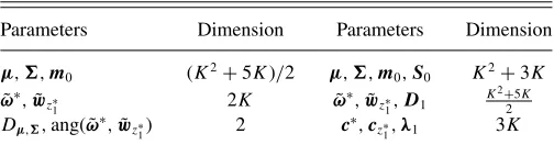
Table 1. Model and prior parameters of thez∗andt∗-tests, respectively, and their dimension

Parameters Dimension Parameters Dimension

μ,,m0 (K2+5K)/2 μ,,m0,S0 K2+3K

˜ ω∗_,w˜

z∗

1 2K ω˜

∗_,w˜

z∗

1,D1

K2_+5K

2

Dμ,,ang( ˜ω∗,w˜z∗

1) 2 c

∗_,c

z∗

1,λ1 3K

The proof of Lemma (4.4) is similar to the proof of Lemma (4.2), albeit rather more complex. The next theorem is direct consequence of Lemmas 4.3 and 4.4.

Theorem 4.3. The design vectord, the vector of eigenvalues λ1of the matrix D1in (4.3),and the vectorscz∗1 andc

∗_{in (4.5)}

are sufficient to determine the power functionβ_t∗.

As we can see inTable 1, the last result reduces the dimension of the design space of thet∗-test substantially, allowing us to explore power across the design space. While the design space, due to the covariance matrix estimation, still depends onK, it is reduced from orderK2_{to orderK.}

Furthermore, this reduction provides an understanding of how the selection of the weighting vector affects power. This be-comes clearer if we consider thatθ_t∗

j in (4.4) can be written as

θt∗

j = cT_z∗

j

−1

j c∗

−1

j cz∗

j

, j =1,2, . . . , J,

where

cz∗

j =

n0cz∗

1+n(j−1)c¯y(j−1)

n0+n(j−1) , j =1+ν(j−1)Scy_(j−1)

+ n0n(j−1)

n0+n(j−1)

c¯y_(j−1)−cz∗₁

c¯y_(j−1)−cz₁∗

T_.

Here, c¯y_(j) and Scy(j) are the sample mean and sample

co-variance matrix of the transformed observation vectorscY(j) =

[cY1cY2. . .cYj] with cY_l, l=1,2, . . . , j, the matrix with

columnscYil =VT1w˜Yil ∼NK(c∗,I),i=1,2, . . . , nj. The last expressions show that the distance of the prior estimatesm0,S0 to the model parametersμ,can be expressed by the distances of the vectorsc_z∗

1andλ

−1

1 =(1/λ11, . . . ,1/λ1K)Ttoc∗, the lat-ter directly reflected to power throughθ_t∗

j (see the next section for more information).

In the special case of the first stage-deviation matrix being proportional to the identity matrix, that is,D1∝ I(λ11=λ12 =

· · · =λ1K), as the next result shows, the design space can be

reduced further.

Theorem 4.4. For D1=c−1I, the design vector d, the constant c, the Mahalanobis distance D_μ,, and the angle ang( ˜w_z∗

1,ω˜

∗_{) are sufficient to determine the power functionβ}

t∗.

The last theorem proves that, for D1∝ I, we can use the fact that the prior-deviation matrix D1 does not change the directions of ˜w_z∗

j’s, to show that the relation ofβt∗to the model parameters and their prior estimates can be described simply by the scalarsD_μ, and ang( ˜w_z∗

1,ω˜

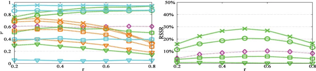
Figure 1. Power (left panel) and RSSR (right panel) versus sample allocation ratio. We plot the sequentialχ2_{-test (magenta··) and the}

z∗_{(green−−line), sequentialz(cyan−), andz}+_{(orange−·) tests with first stage/fixed/first step weighting vector 0 (×), 30}◦_{(◦), 60}◦ ₍₎ and 90◦() angle to the optimal. The remaining design parameters areJ=2,K=10,α=0.05,α_1,1=0.01,α_0,1=1,n_T =60,n0=0.5n1,

Dμ,=0.65.

this result and the results of Theorems 4.2 and 4.3 to perform power analysis studies.

5. EMPIRICAL STUDIES

To explore properties of the adaptivez∗andt∗-tests as well as alternative global tests and to perform comparisons, we present empirical studies making use of the results in Theorems 4.2, 4.3, and 4.4.

In addition toz∗ andt∗-tests, we consider linear combina-tionzandt-tests with fixed weighting vectors, a class that in-cludes the OLSzandt-test in O’Brien (1984). We also consider the likelihood-ratioχ2 _{and Hotelling’sT}2_{-test with statistics}

χ2_=nY¯−1_{Y¯ andT}2_{=n(n−K) ¯Y S}−1

Y Y¯/K(n−1) that

fol-low the noncentralχ2_{andFdistribution withKand (K, n−K)} degrees of freedom, respectively, and noncentrality parameter

D2

μ,. We consider both single stage and sequentialJ-stage de-signs for all these tests. Finally, the two-step, single-stage linear combinationz+andt+tests proposed in Minas et al. (2012) are also considered. Note that the latter tests can be derived as spe-cial cases of thez∗ andt∗-tests forJ =2, (α1,1, α0,1)=(0,1) andC(p2)=p2.

A range of experiments are performed under different values of the design parameters. The power function ofJ-stage (J >1) tests is not analytically tractable and therefore power is approx-imated by the rate of rejections in a large number of simulated replications, hereR=10,000, of a single experiment. Further-more, to study the reduction in sample size due to early stopping of the study, we also empirically compute the rate of sample size reduction (RSSR),

RSSR=100×

nT −E(N)

nT

%,

where n_T =n1+n2+ · · · +nJ the total sample size, N the sample size used for a single replication of the study andE(N) its expected value. Note that single-stage tests have RSSR=0, in contrast to sequential tests that allow for early stopping and thus have nonzero RSSR.

5.1 Simulation Data Examples

We next summarize the main results of a comprehensive study of the power behavior of the above tests in relation to the design parameters (more illustrations are included in Supplementary

Material B). First, larger values of D_μ, and/or n_T result in higher power values for all tests considered, except thezandt -tests with fixed weighting vectors ˜worthogonal to ˜ω∗for which

β =α. Considering the prior sample size, the results indicate that forn0 ∈(0.5n1,0.75n1) the prior estimates become influ-ential, but they do not dominate the accumulated data when selecting the weighting vector while larger values of n0 en-forcesz∗ andt∗ to have more similar behavior tozandt-tests with fixed weighting vector. Furthermore, simulation examples confirm that larger values of the acceptance critical valuesα0,j increase the power of multistage tests especially for larger po-tential power gain in subsequent stages, at the expense of less chance of early acceptance. Simulation examples also confirm that larger power is gained if larger rejection critical valuesα1,j

are allocated to stages with larger potential power gain, while the value of RSSR increases for largerα1,j in early stages.

We also consider power behavior related to allocation of sam-ple size to stages (Figure 1). For the sequentialzandχ2-test, the results show that higher power is achieved if sample allocation is analogous toα-rate allocation. Thez∗ andt∗-tests generally attain higher efficiency for close to balanced allocations. For

˜ wz∗

1 close to (far from) the optimal ˜ω

∗_{, slightly higher power is}

attained for assigning more sample to early (late) stages. Small to moderate allocation ratiosrare more appropriate for thez+ test since noαrate is spent in the first stage. Further, as in the

χ2_{-test, thez}∗_{achieves higher RSSR forr =0.5.}

Before we proceed to comparisons, it is worth consider-ing the impact of being unknown and thus estimated on the performance of the t∗-test. First, in the case of D1∝ I (λ1∝1=(1,1, . . . ,1)T), which as we show in Theorem 4.4 is somewhat easier case to consider, the estimation variability is substantially reduced and thus we generally expect ˜w_t∗

j to be closer to ˜wz∗

j. On the other hand, ifD1∝ I(λ1∝1), the direc-tion ofλ1is more influential on ˜wt∗

j with the consequence being double-edged (see Figure2). That is, compared to the situation of λ1∝1, the distance of ˜w_t∗

j’s to optimal can be larger (left panel) but also smaller (right panel) depending on how close the direction of λ−₁1=(1/λ11, . . . ,1/λ1K)T is to the optimal directionc∗.

Finally, it is useful to note that throughout our simulations of

t∗_{-test, the cos(ang(c}∗_,−1

1 cz∗1)) is shown to be a robust

0.4 0.8 1.2 1.6 0

0.2 0.4 0.6 0.8 1

D

μ,Σ

β

0.4 0.8 1.2 1.6

0 0.2 0.4 0.6 0.8 1

D_μ

,Σ

β

Figure 2. Power of thet∗-test versus Mahalanobis distance for variousc∗,c_z∗

1,λ1. In the left panel, the vectorsc

∗_=c

z∗

1∝1while in the

right panelc∗=e1=(1,0, . . . ,0)T andcz∗

1 ∝1which, forλ1=1(green−×−line), giveϕ=ang(c

∗_,−1

1 cz∗1)=ang(c

∗_,λ−1

1 )=0◦and 72◦,

respectively. In both panels,λ1∝1are also chosen to giveϕ=25◦(dark green−◦−line), 45◦ (dark green−+−line) and 65◦ (dark green −−line). The remaining design parameters areJ=2,K=10,α=0.05,α1,1=0.01,α0,1=1,nT =20,r=0.5,n0=0.75n1,ν0=n0−1.

and their prior estimates. For this reason, but also to reduce com-plexity, in the comparisons to follow, we focus on the case of λ1∝1(particularly, as we explain later on, in cases resembling the right panel of Figure 2), for various values of the summary cos(ang(c∗,−₁1c_z∗

1)).

In terms of comparisons, first note that, for fixed design parameters, single-stage tests attain higher power levels than multi-stage tests, nevertheless at the expense of not allowing for early stopping and thus not allowing for sample size reduction (RSSR=0). Furthermore, it might be useful to emphasize that for fixed design parameters, the power of the linear combination test with weighting vector (either fixed or initial) set equal to the optimal weighting vectorω∗ attains the maximum power and provides an upper bound to all the other presented procedures, including Hotelling’sT2_{-test as proved in Minas et al. (2012)} (Corollary 1). Compared to thez-tests with fixed weighting

vec-torsw, as we can see inFigure 3, the adaptivez∗lose some power for ˜w(=w˜_z∗

1) close to optimal but gains substantial amounts of

power for ˜wfar from optimal, importantly avoiding the problem ofz-tests having zero power for ˜worthogonal to optimal. This result emphasizes that, even though the power of the proposed tests remains sensitive to the prior information used to select the weighting vector, they are less sensitive to the initial selec-tion of the weighting vector than thezandt-tests, where the weighting vector is fixed. The adaptivez∗-test also has substan-tially higher power toz+ for small angles to the optimal and slightly lower power for large angles. Finally, the power of the single-stage and sequentialχ2_{-tests is approximately equal to} the power of thez∗-test for ˜w_z∗

1having respectively 60

◦_{and 45}◦

angle with ˜ω∗. Note that, as the results inFigure 3confirm, all the considered tests control the Type I error at the nominal level

α=0.05.

0 0.4 0.8 1.2 1.6

0 0.2 0.4 0.6 0.8 1

D_μ

,Σ

β

0 0.4 0.8 1.2 1.6

0 0.2 0.4 0.6 0.8 1

D_μ

,Σ

β

0 0.4 0.8 1.2 1.6

0 0.2 0.4 0.6 0.8 1

D_μ

,Σ

β

0 0.4 0.8 1.2 1.6

0% 15% 30% 45% 60% 75%

D_μ

,Σ

RSSR

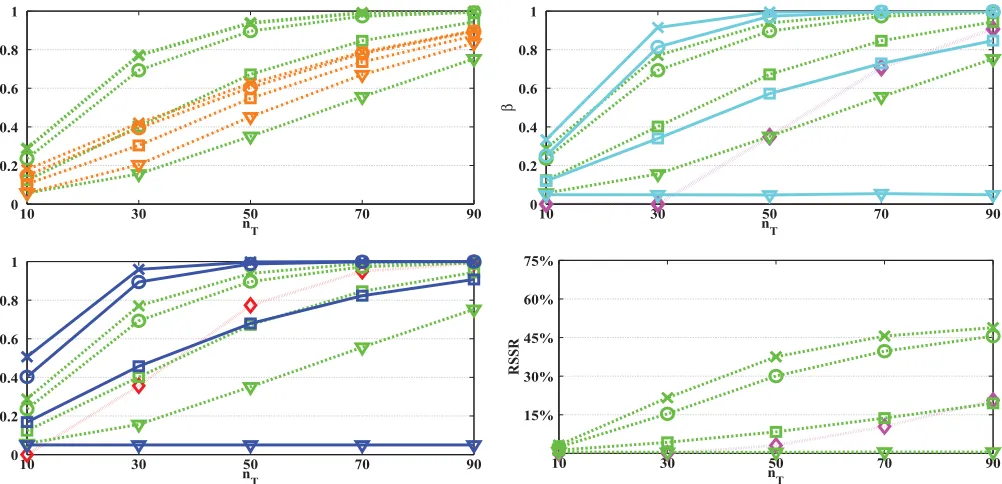
Figure 3. Power and RSSR versus Mahalanobis distance. We plot thez∗-test (green−−) with the testsz+(orange−.) (up left), sequential z(cyan−) andχ2 _{(magenta··) (up right), single stagez(blue−) andχ}2 _{(red··) (down left) and sequentialχ}2 _{(down right). The linear}

10 30 50 70 90 0

0.2 0.4 0.6 0.8 1

n

T

β

10 30 50 70 90

0 0.2 0.4 0.6 0.8 1

n

T

β

10 30 50 70 90

0 0.2 0.4 0.6 0.8 1

n

T

β

10 30 50 70 90

15% 30% 45% 60% 75%

n

T

RSSR

Figure 4. Power and RSSR versus the total sample sizen_T. We plot thet∗-test (green−−) with the tests,t+(orange−.) (up left), sequential t(cyan−) andT2 _{(magenta··) (up right), single staget(blue−) andT}2 _{(red··) (down left) and sequentialT}2 _{(down right). The linear}

combinationt∗/t/t+tests are performed with first stage/fixed/first step weighting vectors having 0 (×), 30◦(◦), 60◦(), and 90◦() angle to the optimal. The remaining design parameters areK=15,J =2,α=0.05,α_1,1=0.01,α_0,1=1,r=0.5,n0=6,ν0=n0−1,Dμ,=0.7.

In the case ofunknown, we consider comparisons for the case ofD1 =Iwhich, using the results of Theorem 4.4, they can be performed in a similar way to the case of known. For the simulations inFigure 4, the case ofD1=Ican be thought of as representative ofλ−₁1fairly distant toc∗(right panel ofFigure 2), since we takec∗ =e1resulting in cos(ang(c∗,λ−11))=

√

K/K

(∼=0.26, angle 75◦, forK=15). As we would expect, the power of all tests is lower than their counterparts forknown (same design parameters), but the patterns of power difference across tests remain the same except from Hotelling’s T2 which in contrast toχ2-test is highly dependent on the sample size.

As Figure 4 illustrates, fornT ≤KornTslightly larger thanK

(here,n_T =10−30 forK=15),T2_{is respectively inapplicable} or very inefficient with power levels lower than the power oft∗ even for angles close to orthogonal. As sample size becomes considerably bigger than K (n_T >50), the power of T2_-test increases sharply to yield power levels analogous to theχ2_-test. For instance, for the design parameters inFigure 4, the single stage and sequentialT2_{-tests, likewise to theχ}2_{-test, have power} close to the power of thet∗for angle 60◦and 45◦, respectively, for large sample sizes.

6. APPLICATION TO AN EEG STUDY

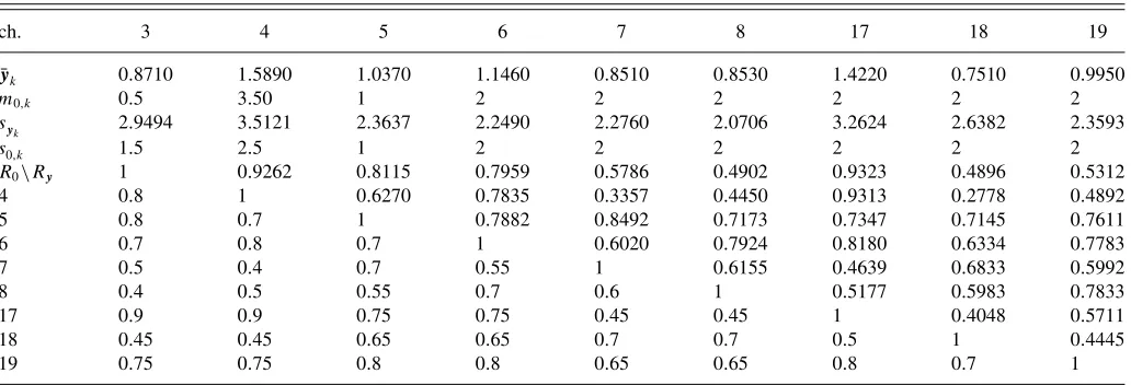
We consider applications to an electroencephalogram (EEG) study, the results of which are provided in L¨auter, Glimm, and Kropf (1996). As L¨auter et al. described, the data are collected fromnT =19 depressive patients at the beginning and at the end of a six week therapy. For demonstration,K =9 variables are used which represent the changes of the absolute theta power in channels 3–8, 17–19 of EEG during the therapy of each pa-tient. In Table 2,we present the means, standard deviations, and

correlation matrix of the data. Note that although an increase is indicated in all channels, none of them (min_kp_k=0.04) fall below the Bonferroni corrected thresholdα/K∼=0.0056 at the

α=5% significance level. Hotelling’sT2_{-test also fails to} re-jectH0 (pT2=0.261). On the contrary, the SS and PCt-tests

proposed by L¨auter et al. rejectH0at the 5% significance level (pSS=0.0489,pPC=0.0487).

We perform power analysis by setting the design parameters as in the above study, that is,n_T =19,K=9,μ=y¯,=S_y,

α=0.05. For these design parameters, the power of Hotelling’s

T2_isβ

T2∼=0.68 (Dμ,=1.15). This is larger than the power

of the SS and PC tests which are respectively βtSS ∼=0.52,

βtPC∼=0.51 (the contrasting results of the tests performed

us-ing these data are because of the different shape of the tand

F distributions). The latter power values are very close to the power of the OLSt-test in O’Brien (1984),β_tOLS ∼=0.52, which

uses the uniform weighting vectorwOLS∝1. This gives angle ang( ˜wOLS,ω˜∗)∼=71◦. Taking into account that the single-stage

t-test for a weighting vector equal to the optimal has power

βt∼=1, we can easily see that there is considerable scope for

improvement.

Table 2. Means, standard deviations, correlations, and their prior estimates for the EEG depression study presented in L¨auter, Glimm, and Kropf (1996)

ch. 3 4 5 6 7 8 17 18 19

¯

y_k 0.8710 1.5890 1.0370 1.1460 0.8510 0.8530 1.4220 0.7510 0.9950

m0,k 0.5 3.50 1 2 2 2 2 2 2

sy_k 2.9494 3.5121 2.3637 2.2490 2.2760 2.0706 3.2624 2.6382 2.3593

s0,k 1.5 2.5 1 2 2 2 2 2 2

R0\Ry 1 0.9262 0.8115 0.7959 0.5786 0.4902 0.9323 0.4896 0.5312

4 0.8 1 0.6270 0.7835 0.3357 0.4450 0.9313 0.2778 0.4892

5 0.8 0.7 1 0.7882 0.8492 0.7173 0.7347 0.7145 0.7611

6 0.7 0.8 0.7 1 0.6020 0.7924 0.8180 0.6334 0.7783

7 0.5 0.4 0.7 0.55 1 0.6155 0.4639 0.6833 0.5992

8 0.4 0.5 0.55 0.7 0.6 1 0.5177 0.5983 0.7833

17 0.9 0.9 0.75 0.75 0.45 0.45 1 0.4048 0.5711

18 0.45 0.45 0.65 0.65 0.7 0.7 0.5 1 0.4445

19 0.75 0.75 0.8 0.8 0.65 0.65 0.8 0.7 1

distances have smaller correlations, with larger correlations set at the highly active frontal regions (in accordance with the literature).

This prior estimate gives ang( ˜wt∗

1,ω˜

∗_)=37.27◦ _{which is}

much smaller than the angle under the uniform weighting vector. For a two-stage design (J =2), with balanced sam-ple allocation,n1=10,n2=9, andαallocationα1,1=0.01,

a2=0.0087, no early acceptance allowed,α0,1=1, prior sam-ple sizen0=7=0.7n1,ν0=6 (see previous section) and the remaining design parameters as the original study, thet∗-test has powerβ_t∗∼=0.84 with RSSR=∼22.3% (E(N)∼=15).

Sub-stantial power improvement is also obtained over thet+which, forn0=6,n1=13,n2=6 (r=0.3) and the remaining design parameters as above, has powerβ_t+ ∼=0.64.

7. DISCUSSION

The methods developed in this work demonstrate that lin-ear combination tests provide a substantial alternative to the classical Hotelling’s T2 _{global test, especially in the setting,} commonly encountered in recent important applications of clin-ical neuroscience, of the available sample sizen being small compared to the observation dimension K. It is also shown that adaptive linear combination tests provide power robustness across the set of alternative hypotheses since they can correct initial selections of the weighting vector which are far from the optimal selection. The adaptiveJ-stagez∗andt∗-tests achieve high power levels for largen, independently of the initial selec-tion of weighting vector, but most importantly they can achieve high-power performance even ifnis limited.

The proposed tests achieve optimality in the sense of max-imizing the predictive power of the test at each interim anal-ysis. Predictive power has been used for sample size calcula-tion (O’Hagan and Stevens2001), treatment selection (Kimani, Stallard, and Hutton 2009) and to select the component-wise significance levels in multiple testing (Westfall, Krishen, and Young 1998). It is a useful tool for incorporating prior infor-mation into the design of a study, particularly as such studies can often be viewed as a decision-making process. The appli-cation in Section6provides an example of a setting in which

prior information is available and can substantially improve the performance of existing tests.

Optimality is attained in our methods without undermining the two main targets of adaptive designs: flexibility and test specificity. This allows for future developments of the proposed test to consider further optimal design adaptations. The use of other adaptive designs techniques, such as sample size re-assessment, within our methodology can improve further the performance of the proposed tests.

The power characterization in Section4provides a tool for understanding and alleviating to some extent the complexities of multivariate tests especially those based on response dimen-sion reductions. The possibly high-dimendimen-sional model param-eters and their prior estimates are reduced to low-dimensional summaries which are still sufficient to compute power. Impor-tantly, these summaries have interpretations directly related to the strength of the treatment effect and the effect of the dimen-sion reduction on power. They provide a method for performing simple power analysis, but also understanding the behavior of linear combination tests.

The methods used to derive the power characterization are also interesting in their own right. They can be generally de-scribed by two steps: standardization and rotation invariance. The first standardization step is a prevalent technique for reex-pressing statistical models in the standard deviation unit and eliminating correlations. Here, it allows us to reexpress the weighting vector selection, which involves estimating the un-known model parameters, as a procedure of learning a single vector, that is, the optimal weighting vector. The second step of establishing a rotation invariance property for the power func-tion allows us to identify the measure quantifying the angular distance between the selected and the optimal weighting vector, reducing further the design space. The question whether these results can be derived under more relaxed modeling assumptions is an area of ongoing research.

SUPPLEMENTARY MATERIALS