Satisfiability-Based Algorithms for Boolean Optimization
Vasco M. Manquinho ([email protected]) Dept. of Informatics, Technical University of Lisbon IST/INESC
Lisbon, Portugal
Jo˜ao P. Marques-Silva ([email protected]) Dept. of Informatics, Technical University of Lisbon IST/INESC/Cadence European Labs.
Lisbon, Portugal
Abstract.
This paper proposes new algorithms for the Binate Covering Problem (BCP), a well-known restriction of Boolean Optimization. Binate Covering finds application in many areas of Computer Science and Engineering. In Artificial Intelligence, BCP can be used for computing minimum-size prime implicants of Boolean functions, of interest in Automated Reasoning and Non-Monotonic Reasoning. Moreover, Binate Covering is an essential modeling tool in Electronic Design Automation. The ob-jectives of the paper are to briefly review branch-and-bound algorithms for BCP, to describe how to apply backtrack search pruning techniques from the Boolean Satisfiability (SAT) domain to BCP, and to illustrate how to strengthen those prun-ing techniques by exploitprun-ing the actual formulation of BCP. Experimental results, obtained on representative instances indicate that the proposed techniques provide significant performance gains for a large number of problem instances.
Keywords:Binate Covering Problem, Propositional Satisfiability, Branch-and-Bound, Backtrack Search, Non-Chronological Backtracking
1. Introduction
In recent years, several powerful search pruning techniques have been proposed for solving BCP, allowing dramatic improvements in the ability to solving large and complex instances of BCP. (Details of the work on BCP can be found in [4, 12, 20].) Despite these improvements, and as with other NP-hard problems, additional search pruning ability allows in general very significant gains, both in the amount of search and in the run times. The ultimate consequence of proposing new pruning techniques is the potential ability for solving new classes of instances.
The main objective of this paper is to propose additional tech-niques for pruning the amount of search in branch-and-bound algo-rithms for solving binate covering problems. These techniques cor-respond to generalizations and extensions of similar techniques pro-posed in the Boolean Satisfiability (SAT) domain, where they have been shown to be highly effective [2, 17, 22]. In particular, and to our best knowledge, we provide for the first time conditions which enable branch-and-bound algorithms to backtrack non-chronologically whenever bounding due to the cost function is required to take place. Although our main focus is on one particular bounding mechanism (maximum independent set of clauses), we also establish conditions for non-chronological backtracking with other bounding procedures.
The paper is organized as follows. In Section 2 the notation used throughout the paper is introduced. Afterwards, branch-and-bound covering algorithms are briefly reviewed, giving emphasis to solutions based on SAT algorithms and in section 4 different bounding procedures are also described. In subsequent sections, we propose new techniques for reducing the amount of search. In particular we show how effective search pruning techniques from the SAT domain can be generalized and extended to the BCP domain. Experimental results are presented in Section 8, and the paper concludes in Section 9.
2. Preliminaries
An instance C of a covering problem is defined as follows,
minimize Pn j=1
cj ·xj
subject to A·x≥b, x∈ {0,1}n
(1)
wherecj is a non-negative integer cost associated with variablexj,1≤
j ≤nandA·x≥b, x∈ {0,1}n denote the set ofmlinear constraints. If every entry in the (m×n) matrixAis in the set{0,1}and bi= 1,1≤
Moreover, if the entriesaij ofAbelong to{−1,0,1}andbi = 1− |{aij :
aij = −1,1 ≤ j ≤ n}|, then C is an instance of the binate covering problem (BCP). Observe that ifC is an instance of the binate covering problem, then each constraint can be interpreted as a propositional clause.
Conjunctive Normal Form (CNF) formulas are introduced next. The use of CNF formulas is justified by noting that the set of constraints of an instance C of BCP is equivalent to a CNF formula, and because some of the search pruning techniques described in the remainder of the paper are easier to convey in this alternative representation.
A propositional formula ϕ in Conjunctive Normal Form (CNF) denotes a boolean function f :{0,1}n→ {0,1}. The formula ϕ con-sists of a conjunction of propositional clauses, where each clauseω is a disjunction of literals, and a literal lis either a variable xj or its com-plement ¯xj. If a literal assumes value 1, then the clause issatisfied. If all literals of a clause assume value 0, the clause isunsatisfied. Clauses with only one unassigned literal are referred to asunit. Finally, clauses with more than one unassigned literal are said to beunresolved. In a search procedure, a conflictis said to be identified when at least one clause is unsatisfied. In addition, observe that a clauseω = (l1+· · ·+lk), k≤n, can be interpreted as a linear inequality l1 +· · ·+lk ≥ 1, and the complement of a variable xj, ¯xj, can be represented by 1−xj.
When a clause is unit (with only one unassigned literal) an assign-ment can be implied. For example, consider a propositional formula ϕ
which contains clauseω= (x1+ ¯x2) and assume thatx2 = 1. Forϕto be satisfied, x1 must be assigned value 1 due to ω. Therefore, we say that
x2= 1impliesx1 = 1 due toωor that clauseωexplainsthe assignment
x1= 1. These logical implications correspond to the application of the unit clause rule [7] and the process of repeatedly applying this rule is called boolean constraint propagation [17, 22]. It should be noted that throughout the remainder of this paper some familiarity with backtrack search SAT algorithms is assumed. The interested reader is referred to the bibliography (see for example [1, 17] for additional references).
3. Search Algorithms for Covering Problems
The most widely known approach for solving covering problems is the classical branch-and-bound procedure [20], in which upper bounds on the value of the cost function are identified for each solution to the constraints, and lower bounds on the value of the cost function are estimated considering the current set of variable assignments. The search can be pruned whenever the lower bound estimate is higher than or equal to the most recently computed upper bound. In these cases we can guarantee that a better solution cannot be found with the current variable assignments and therefore the search can be pruned. The algorithms described in [5, 12, 20] follow this approach.
Several lower bound estimation procedures can be used, namely the ones based on linear-programming relaxations [12], Lagrangian relaxations [16] or the Log-approximation approach [4]. Nevertheless, and for BCP, the approximation of a maximum independent set of clauses [4] is the most commonly used. The tightness of the lower bounding procedure is crucial for the algorithm’s efficiency, because with higher estimates of the lower bound, the search can be pruned earlier. For a better understanding of lower bounding mechanisms, dif-ferent methods will be described. We will address linear programming relaxations, the Log-approximation approach, and will emphasize the approximation of the maximum independent set of clauses. Covering algorithms also incorporate several powerful reduction techniques, a comprehensive overview of which can be found in [4, 20].
With respect to the application of SAT to Boolean Optimization, P. Barth [1] first proposed a SAT-based approach for solving pseudo-boolean optimization (i.e. a generalization of BCP). This approach consists of performing a linear search on the possible values of the cost function, starting from the highest, at each step requiring the next computed solution to have a cost lower than the most recently com-puted upper bound. Whenever a new solution is found which satisfies all the constraints, the value of the cost function is recorded as the current lowest computed upper bound. If the resulting instance of SAT is not satisfiable, then the solution to the instance of BCP is given by the last recorded solution.
int bsolo(ϕ) { ub=Pcj+ 1;
while (TRUE) {
decide();
if (!consistent state()) return ub;
while (Estimate LB() ≥ ub) {
Issue LB based conflict(); if (!consistent state())
return ub;
} } }
int consistent state() {
while (Deduce() == CONFLICT) if (Diagnose() == CONFLICT)
return FALSE; if (Solution found())
Update ub(); return TRUE;
[image:5.612.216.375.47.276.2]}
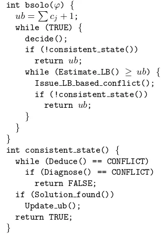
Figure 1. SAT-based branch-and-bound algorithm
branch-and-bound algorithms, and the search pruning techniques from SAT algorithms.
The algorithm presented in [14] already incorporates the main pruning techniques of the GRASP SAT algorithm [17]. Hence, bsolo is a branch-and-bound algorithm for solving BCP that implements a non-chronological backtracking search strategy, clause recording and identification of necessary assignments. Mainly due to an effective con-flict analysis procedure which allows non-chronological backtracking steps to be identified, bsolo performs better than other branch-and-bound algorithms in several classes of instances, as shown in [14]. However, non-chronological backtracking is limited to one specific type of conflict. In section 5 we describe how to apply non-chronological backtracking to alltypes of conflicts when using the approximation of a maximum independent set of clauses. Moreover, in section 7 we also describe how to apply the same concepts when using other lower bound estimation methods.
The main steps of a simplified version of thebsolo algorithm (see fig. 1) can be described as follows:
1. Initialize the upper bound to the highest possible value as defined (i.e. given byub=Pn
2. The function consistent state starts by checking whether the cur-rent state yields a conflict. This is done by applying boolean con-straint propagation and, in case a conflict is reached, by invok-ing the conflict analysis procedure, recordinvok-ing relevant clauses and proceeding with the search procedure or backtrack if necessary.
3. If a solution to the constraints has been identified, update the upper bound according to ub=Pnj=1cj·xj. (Observe that the only way to reduce the value of the current solution is to backtrack with the objective of finding a solution with a lower cost.)
4. Estimate a lower bound given the current variable assignments. If this value is higher than or equal to the current upper bound, issue a bound conflict and bound the search by applying the conflict analysis procedure to determine which decision node to backtrack to (using functionconsistent state). Continue from step 2.
3.1. Bound Conflicts
In bsolo two types of conflicts can be identified: logical conflicts that occur when at least one of the problem instance constraints becomes unsatisfied, and bound conflicts that occur when the lower bound is higher than or equal to the upper bound. When logical conflicts occur, the conflict analysis procedure from GRASP is applied and determines to which decision level the search should backtrack to (possibly in a non-chronological manner).
However, the other type of conflict is handled differently. Inbsolo, whenever a bound conflict is identified, a new clause mustbe added to the problem instance in order for a logical conflict to be issued and, consequently, to bound the search. This requirement is inherited from the GRASP SAT algorithm where, for guaranteeing completeness, both conflicts and implied variable assignments must be explained in terms of the existing variable assignments [17]. With respect to conflicts, each recorded conflict clause is built using the assignments that are deemed responsible for the conflict to occur. If the assignment xj = 1 (orxj = 0) is considered responsible, the literal ¯xj (respectively, literal xj) is added to the conflict clause. This literal basically states that in order to avoid the conflict one possibility is certainly to have instead the assignment xj = 0 (respectively, xj = 1). Clearly, by construction, after the clause is built its state is unsatisfied. Consequently, the conflict analysis procedure has to be called to determine to which decision level the algorithm must backtrack to. Hence the search is bound.
variables in the search tree. In this case, the conflict would always depend on the last decision variable. Therefore, backtracking due to bound conflicts would necessarily be chronological (i.e. to the previ-ous decision level), hence guaranteeing that the algorithm would be complete. Suppose that the set {x1 = 1, x2 = 0, x3 = 0, x4 = 1} corresponds to all the search tree decision assignments and ωbc is the clause to be added due to a bound conflict. Then we would have
ωbc= (¯x1+x2+x3+ ¯x4). Again, the drawback of this approach (which was used in [14]) is that backtracking due to bound conflicts is always chronological, since it depends on all decision assignments made. In section 5 we propose a new procedure to build these clauses, which enables non-chronological backtracking due to bound conflicts.
4. Computation of Lower Bounds
The estimation of lower bounds on the value of the cost function is a very effective method to prune the search tree and the accuracy of lower bounding procedures is critical for identifying areas of the search space where solutions to the constraints with lower values of the cost function cannot be found. In this section we review methods commonly used to estimate a lower bound on the value of the cost function in instances of BCP.
4.1. Maximum Independent Set of Clauses
The maximum independent set of clauses (MIS) is a greedy method to estimate a lower bound on the value of the cost function based on an independent set of clauses. (A more detailed definition can be found for example in [4]).
The greedy procedure consists of finding a set M IS of disjoint unate clauses, i.e. clauses with only positive literals and with no literals in common among them. Since maximizing the cost of M IS is an NP-hard problem, a greedy computation is used, as shown in fig. 2. The effectiveness of this method largely depends on the clauses included in M IS. Usually, one chooses the clause which maximizes the ratio between its weight and its number of elements.
The minimum cost for satisfying M IS is a lower bound on the solution of the problem instance and is given by,
Cost(M IS) = X ω∈M IS
W eight(ω) where (2)
W eight(ω) = min xj∈ω
maximal independent set(ϕ) {
MIS = ∅; do{
ω = choose clause(ϕ); MIS = MIS ∪ {ω};
ϕ = delete intersecting clauses(ϕ,ω);
} while (ϕ6=∅); return MIS;
}
Figure 2. Algorithm for computing a MIS
4.2. Linear Programming Relaxations
Linear programming relaxations have long been used as lower bound estimation procedures in branch-and-bound algorithms for solving in-teger programming problems [16]. For the binate covering problem, the utilization of linear programming relaxations as a lower bound estimation method is proposed in [12]. Moreover, it is also claimed that in most cases the linear programming relaxation (LPR) bound is higher than the one obtained with the MIS approach.
The general formulation of the LPR for a covering problem is obtained from (1) as follows:
minimize zlpr= n
P
j=1
cj ·xj
subject to A·x≥b x≥0
(4)
For simplicity the constraints x ≤ 1 are not included. The solution of (1) is referred to as z∗
cp, whereas the solution of (4) is referred to as
z∗ lpr.
It is well-known that the solution z∗
lpr of (4) is a lower bound on the solution z∗
cp of (1) [16]. Basically, any solution of (1) is also a feasible solution of (4), but the converse is not true. Moreover, for a given solution of (4) where x∈ {0,1}n, we necessarily havez∗
cp =z∗lpr. Hence, the result follows. Furthermore, different linear programming algorithms can be used for solving (4), some of which with guaranteed worst-case polynomial run time [16].
4.3. Log-Approximation
greedy solution(ϕ) {
SOL = ∅; while (ϕ6=∅) {
var = minvar∈V ar(ϕ)
Cost(var) Γ(cov clauses(var, ϕ));
ϕ=ϕ−cov clauses(var, ϕ); SOL = SOL ∪ var;
}
return SOL;
[image:9.612.190.399.49.157.2]}
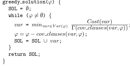
Figure 3. Algorithm for computation of a greedy solution
poor quality, tighter lower bounds can be established. In [5] a new lower bound computation algorithm for unate covering is introduced which guarantees a logarithmic ratio bound on the minimum cost solution.
The algorithm in Fig. 3 describes a procedure for constructing a greedy solution for a covering problem with a set ϕ of constraints to satisfy. At each step a decision variable var is chosen, the clauses that become satisfied by var are removed from ϕ and a solution set is updated. Observe that the algorithm was conceived to tackle unate covering problems [5], but it can be easily modified in order to attempt to find greedy solutions for binate covering instances1. The variable to add to the solution set is the one which minimizes the relation between its cost and the value given by Γ. Letγ be a positive weighting function defined on a set of clauses (e.g. the number of free literals). We can define Γ as:
Γ(ϕ′
) = X
ω∈ϕ′
γ(ω) (5)
It can be shown [5] that based on the greedy solution given by the algorithm in Fig. 3, it is possible to obtain a lower bound on the covering problem which is log-approximable to the optimum value
z∗
cp. This result is also valid for binate covering whenever the greedy algorithm is able to find a feasible solution. The lower bound is given by:
Cost(SOL)
r (6)
where r=
maxϕ′Γ(ϕ′)
X
k=1
1/k (7)
1 In binate covering, the greedy algorithm is unable to guarantee that a solution
5. SAT-Based Pruning Techniques for BCP
One of the main features of bsolo is the ability to backtrack non-chronologically when conflicts occur. This feature is enabled by the conflict analysis procedure inherited from the GRASP SAT algorithm. However, as illustrated in section 3.1, in the original bsolo algorithm non-chronological backtracking was only possible for logical conflicts. In the case of a bound conflict all the search tree decision assignments were used to explain the conflict. Therefore, these conflicts would always depend on the last decision level and backtracking would necessarily be chronological.
In this section we describe how to compute sets of assignments that explain bound conflicts. Moreover, we show that these assignments are not in general associated with all decision levels in the search tree; hence non-chronological backtracking can take place.
A bound conflict in an instance of the binate covering problem (BCP) C arises when the lower bound is equal to or higher than the upper bound. This condition can be written as C.path+C.lower ≥ C.upper, where C.path is the cost of the assignments already made, C.lower is a lower bound estimate on the cost of satisfying the clauses not yet satisfied (as given for example by an independent set of clauses), and C.upperis the best solution found so far. From the previous equa-tion, we can readily conclude that C.path and C.lower are the unique components involved in each bound conflict. (Notice thatC.upperis just the lowest value of the cost function for the solutions of the constraints computed earlier in the search process.) Therefore, we will analyze both C.path and C.lower components in order to establish the assignments responsible for a given bound conflict.
We start by studyingC.path. Clearly, the variable assignments that cause the value of C.path to grow are solely those assignments with a value of 1. Hence, we can define a set of literals ωcp, such that each variable in ωcp has positive cost and is assigned value 1:
ωcp={l= ¯xj :Cost(xj)>0∧xj = 1} (8)
which basically states that to decrease the value of the cost function (i.e. C.path) at least one variable that is assigned value 1 has instead to be assigned value 0.
0. If any of these literals was assigned value 1, ωi would certainly not be in M IS since it would be a satisfied clause. Consequently, we can define a set of literals that explain the value of C.lower:
ωcl ={l:l= 0∧l∈ωi∧ωi ∈M IS} (9)
Now, as stated above, a bound conflict is solely due to the two compo-nents C.path and C.lower. Hence, this bound conflict will hold as long as the following clause ωbc is unsatisfied:
ωbc=ωcp∪ωcl (10)
(Observe that the set union symbol in the previous equation denotes a disjunction of literals.) As long as this clause is unsatisfied, the val-ues of C.path and C.lower will remain unchanged, and so the bound conflict will exist. We can thus use this unsatisfied clause ωbc to an-alyze the bound conflict and decide where to backtrack to, using the conflict analysis procedure of GRASP [17]. We should observe that backtracking can be non-chronological, because clause ωbc does not necessarily depend on all decision assignments. Moreover, due to the clause recording mechanism,ωbccan be used later in the search process to prune the search tree. If these clauses would depend on all decision assignments, clause recording would not be used since the same set of decision assignments is never repeated in the search process.
Bound conflicts arise during the search process whenever we have
C.path+C.lower≥C.upper. Notice that when a new solution is found,
C.lower = 0 because the independent set is empty (all clauses are satisfied) andC.pathis equal to the cost of the new upper bound. There-fore, when we update C.upper with the new value, we have C.path+
C.lower=C.upper and a bound conflict is issued in order to backtrack in the search tree. These bound conflicts are just a particular case and the same process we described in this section is applied in order to build the conflict clause.
6. Reducing Dependencies in Bound Conflicts
non-chronologically. Hence, after computing explanations for bound conflicts, using the techniques described in the previous section, the next step is to identify assignments that can be discarded from each explanation by proving them irrelevant for the bound conflict to take place.
In this section we propose different techniques for reducing de-pendencies in the explanations of bound conflicts, hence reducing the number of literals inωbc.
6.1. Relating C.path and C.lower
Let lj be a literal such that lj ∈ ωcp and lj 6∈ ωcl. Then lj is in ωbc only due to the C.path component explaining the bound conflict. Let MIS be the independent set, computed with the procedure described in fig. 2, which is used to obtain the value ofC.lower. In this situation, literal lj can be removed from ωcp provided the following conditions apply:
− There exists a satisfied clause ωi such that ¯lj is the only literal which currently satisfiesωi.
− All literals ofωi besideslj must be positive, unassigned and must not intersect MIS (so that ωi can be added to MIS if lj assumes value 0).
− All literals inωi must have a cost higher than or equal to the cost of literal lj.
− No clause inMIS contains lj.
This reduction step can be made because if lj = 0, ωi would be in the independent set and the lower bound value would not decrease. Therefore, literal lj can be deemed irrelevant for explaining the bound conflict and can be removed fromωbc.
As an example, let us suppose that variablesx1,x2 andx3 belong to the cost function with the same cost andx1 = 1. If a bound conflict occurs, from (8) ¯x1 would be in ωbc. However, suppose that clause
ωi = (x1 +x2 +x3) is satisfied only due to x1, i.e., x2 and x3 are unassigned. If x2 and x3 do not belong to any clause in M IS, ¯x1 can be removed from ωbc becausex1 = 1 is not relevant for the conflict. If variable x1 was unassigned or assigned value 0, ωi would be in M IS and the bound conflict would still occur.
Letx1 = 1 andx2 = 0. Moreover, let the cost ofx1 be no greater than the cost of x2, let x3, x4 be such that ωi would be in MIS if x1 = 0, and let no other clause in MIS contain literal x2. In this situation, the dependency on x1 can be removed, and the dependency onx2need not be considered. Indeed, withx1 = 0,ωi would be inMIS and so the cost would not decrease. In addition, since the cost of x2 is larger than or equal to the cost of x1, by assigning value 1 tox2, the cost would also not decrease. Hence the result follows. One should note that the same reasoning applies for an arbitrarynumber of variables assigned value 0 in a given clause with a single literal assigned value 1.
Next we show how ωcl can be simplified by evaluating the conse-quences of modifying the value of some literals on the value of C.path. Suppose we have a literal l = xj, with l ∈ ωcl and let xj = 0. If
xj only belongs to one clause ωi of the independent set and its cost is greater than or equal to the minimum cost ofωi, thenlcan be removed from ωbc. To better understand how this is possible, suppose instead that xj = 1. In this situation, ωi would not be in the independent set (it would be a satisfied clause) and the C.lower component would be lower2. However, since the cost of the variable is higher than or equal to the minimum cost of ωi, the C.path component would be higher, and hence the conflict would still hold. So, the assignment xj = 0 is irrelevant for the conflict to arise and literal l can be removed from
ωbc. Observe that the same reasoning still applies even if a clause ωi, containing literalxj = 0, contains any number of other literals assigned value 0.
Another reduction technique consists of using a satisfied clause to reduce a dependency from ωcl. Let us consider the following set of clauses,
ω1 = (x1+x2+x3)
ω2 = (x1+x4+x5)
ω3 = (x1+x3+x4)
(11)
with x1 = 0, x2, x3, x4, x5 unassigned, and let ω1 and ω2 be part of MIS. Let the cost of x2, x3, x4, x5 be less than or equal to the cost of x1. Finally, let no other clause in MIS contain x1. If x1 would be assigned value 1, C.lower would decrease by 1 since ω1 and ω2 would be satisfied, but ω3 would now be in MIS. However, C.path would be raised due to the cost of x1 and the conflict would still hold. Hence, the dependency on x1 can be removed.
2 In fact, if theC.lowerwould be recomputed all over again, it is not guaranteed
that it would decrease. Nevertheless, we know that without clause ωi satisfied by xj = 1,M IS\{ωi} it is still an independent set of clauses. Therefore,M IS\{ωi}
6.2. Using Excess Cost Value
Let us consider a bound conflict and let diff = (C.path+C.lower)− C.upper. Clearly, diff ≥0.
It is plain that if C.path was lower by diff, the bound conflict would still hold since we would then haveC.path+C.lower=C.upper. Therefore, we may conclude that not all assignments in C.path are necessary for explaining the conflict, since if some assignments were not made, we would still have a bound conflict. In this case, it is possible to remove some literals from ωcp as long as their cost is lower than or equal to diff.
Moreover, the value ofdiff can also be used for reducing dependen-cies fromC.lower. Notice that if we remove a subset of clausesD M IS
from M IS (used to obtainC.lower) such that,
Cost(D M IS)≤diff where (12)
Cost(D M IS) = X ω∈D M IS
W eight(ω) (13)
then the lower bound conflict will still hold since C.path+C.lower ≥ C.upper, where C.lower is now obtained from the independent set of clauses M IS\D M IS. Therefore, the lower bound conflict clause ωbc can still be built using (10), but ωcl can now be reformulated as
ωcl={l:l= 0∧l∈ωi∧ωi∈M IS\D M IS} (14)
Moreover, the simplifications described above forωclcan now be applied to the resulting ωcl.
One should note that the reduction of the number of dependencies relies on which clauses we choose to include in D M IS. If a clause fromM IS is selected with assigned literals belonging toωbcbecause of other clauses in M IS or due toωcp, then the dependencies are exactly the same. Therefore, it is desirable that D M IS be a subset of M IS
such that the number of dependencies in ωbc be minimum. Currently, inbsolo, a greedy procedure is used for selecting the clauses to remove from M IS.
6.3. Resolution-Induced Dependency Reduction
The conditions proposed subsequently can be applied to removing dependencies fromωcpandωcl. In all cases, we use examples to illustrate the application of resolution, but provide the necessary conditions for generic application.
We start by studying simplifications to ωcp established with the resolution operation. Let us consider the following set of clauses,
ω1 = (x1+x2+x3)
ω2 = (x1+x2+x4) (15)
with x2 = 1, and such that x3, x4 are not covered by the currently computedMIS.x1can either be assigned or unassigned, and can either be or not be covered by the currently computedMIS. By applying res-olution between ω1 and ω2, with respect tox1, we obtain the resulting clauseω3 =c(ω1, ω2, x1) = (x2+x3+x4). Now,ω3is certainly satisfied solely by x2. Hence, we can conclude that the dependency onx2 can be removed by applying the results of sections 6.1 and 6.2 on simplifying
ωcp. Notice that x1 can be any variable. However, if x1 is unassigned and not covered byMIS, then we can immediately apply the previous results on simplifying ωcp.
Next, we illustrate one additional form of using the resolution operation for removing dependencies. As an example, assume a bound conflict, and consider the following set of clauses,
ω1 = (x1+x2+x3)
ω2 = (x1+x4+x5) (16)
wherex1 is assigned either value 0 or 1, its cost is 0, and such that the dependency on x1 is only due toω1 orω2. Furthermore, let us assume that ω1 would be part of MIS withx1 = 0, and thatω2 would be part of MIS with x1 = 1. In this situation the dependency on x1 can be removed. Notice that if the cost of x1 is non-zero, then the removal of the dependency onx1is guaranteed by the previous results (section 6.1) on simplifying ωcl.
Clearly, the application of the resolution operation can be general-ized and used for eliminating more than one variable, the only drawback being the computational effort involved.
7. Bound Pruning with Other Lower Bound Methods
equal to the best solution found so far. Notice that in the first case, the procedure does not depend on the method used for computing the lower bound3, whereas in the second case it is assumed that the lower bound computation method is the maximum independent set (MIS) described in section 4.1. If a different lower bound estimation procedure is used, the techniques proposed so far to allow non-chronological backtrack-ing cannot be utilized, since a different procedure will be required for identifying an explanation for the bound conflict. In the remainder of this section we present a theoretical framework which also allows non-chronological backtracking when the other lower bounding procedures described in section 4 are used.
7.1. Pruning with LP-Relaxation Lower Bounds
Linear programming relaxations (LPR) are a powerful method to esti-mate a lower bound value for binate covering instances [12]. However, the resulting backtrack from a bound conflict when using LPR has always been chronological. As mentioned previously, the techniques presented in sections 5 and 6 are useless since the application of the MIS procedure is assumed. The naive approach to build a clause to bound the search in bound conflicts when using LPR would be to include all decision variables in the search tree. However, as stated in sec-tion 3.1, the resulting backtrack would necessarily be chronological. In this section, we present a new framework that allows non-chronological backtracking in bound conflicts when linear programming relaxations are used to estimate the lower bound value.
Remember that a bound conflict occurs whenC.path+C.lower≥ C.upper, in which case a set of assignments that explains the conflict must be identified. Therefore, we must identify the assignments that explain the value onC.path(ωcp) andC.lower(ωcl) in order to build the bound conflict clauseωbc to bound the search. Notice that the value on
C.pathis independent on the lower bound computation procedure and it can be build as described in section 5. However, not every reduction technique presented in section 6 can be applied to ωcp, since some of these techniques depend on the fact that the MIS procedure is used to compute C.lower.
The approach to build ωcl must be different from what was pre-sented in section 5 , since C.lower depends on the value given by the LP-solver. Therefore, the information provided by the LP-solver must be used in order to implement a non-chronological backtracking
3 When a new solution is found, all clauses are satisfied and the lower bound
search strategy in a lower bound conflict when using LPR for bound computation.
Given the value ofC.lowerusing LPR as formulated in section 4.2, let S be the set of constraints withslack 4 variables assigned value 0. Observe that these are the constraints which actually limit the value of C.lower, and so will be referred to as the active constraints. When using LP-relaxations to obtain the value of C.lower, the literals that assume value 0 in the active constraints are directly responsible for its value. These literals correspond to the set ωcl in the bound conflict clause. Applying this reasoning to both assignments of a given variable, allows implementing non-chronological backtracking.
We now illustrate how non-chronological backtrack is possible when using LPR. Let C.lower be computed using LP-relaxations and let
dLP R denote the highest decision level, besides the current decision level, of the zero-valued literal assignments in the constraints for which the slack variables assume value 0. Let the current decision level be
d+kand let dbe the lowest decision level such that,
C.path(d) +Cl.lower(d+k)≥C.upper (17)
C.path(d) +Cr.lower(d+k)≥C.upper (18)
The highest decision levels involved, besides the current decision level
d+kare, respectively,dLP R,lfrom (17) anddLP R,rfrom (18). In this
sit-uation, the search process can backtrack to decision levelmax{d, dLP R,l, dLP R,r}. Observe that the highest decision level in max{d, dLP R,l, dLP R,r}
de-notes the first possibility for one of the constraints in (17) or (18) not to hold. Hence, the search process can safely and non-chronologically backtrack to this decision level.
7.2. Pruning with Log-Approximation Lower Bounds
When C.lower is estimated using the Log-approximation method de-scribed in section 4.3, its value depends on the variable assignments chosen by the greedy algorithm (see Fig. 3). Notice that each time a variable assignment is chosen, it depends on the value of function Γ. Therefore, choosing a variable assignment depends on the clauses which become satisfied with that assignment.
Suppose an assignment to variable xj is chosen at iteration k of the greedy algorithm. This assignment is due to the fact that there is a set of clauses given by cov clauses(xj, ϕ(k)′)5 which become satisfied
4 See [3] for a definition of slack and artificial variables. 5 Notice thatϕ(k)′
and this set of clauses allows variable xj to be chosen by the algo-rithm. Therefore, the clauses in cov clauses provide an explanation for the assignment to variable xj. Moreover, the literals assigned value 0 in cov clauses(xj, ϕ(k)′) are the ones deemed responsible since if they were to have a different value, cov clauses(xj, ϕ(k)′) would be a smaller set which could cause the assignment to variable xj unrequired and hence C.lower could be lower. Notice that if any of the literals considered responsible were to satisfy some of these clauses by having the opposite value, the set of clauses to satisfy (given by cov clauses) would be smaller and a lower value for C.lower could be obtained, possibly solving the bound conflict situation.
Let C.lower be estimated using the Log-approximation method and letSOL be the solution found by the greedy algorithm inn itera-tions which yields a bound conflict. In that case, a bound conflict clause
ωbcmust be created to bound the search. The explanation onC.pathis determined as described previously in section 5, since it does not depend on the lower bound estimation method. Moreover, the explanation on
C.lower is given by:
ωcl ={l:l= 0∧l∈ωi∧ωi ∈π(n)} (19)
where π(n) is the set of all clauses covered by the assigned variables chosen until iteration nwhich is equivalent to:
π(n) =cov clauses(SOL[1], ϕ(1)′
)∪...∪cov clauses(SOL[n], ϕ(n)′ ) (20) where SOL[k] is the selected assignment at iteration k in the greedy algorithm.
Notice that at iteration nall clauses from ϕ(clauses that are not yet satisfied) are in π(n), since all are covered at iteration n of the greedy algorithm. Nevertheless, it is possible that the resulting bound conflict clauseωbcdoes not depend on the last decision assignment level and non-chronological backtracking can take place.
8. Experimental Results
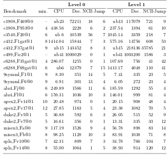
the algorithm was unable to solve the instance due to time restrictions, the best upper bound found at the time is shown. Otherwise, if no upper bound was computed, the reason of failure is shown, which was either due to the time (time) or memory (mem.) limits imposed. In Tables I and II, besides the time taken and the number of decisions made to solve the instances, it is also shown the number of non-chronological backtracks and the highest jump made in the search tree.
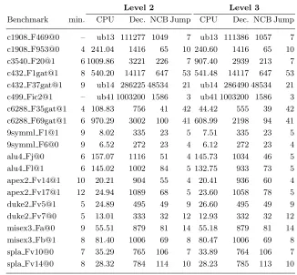
The experimental procedure consisted of running a selected set of problem instances with the bsoloalgorithm, as described in Sections 3, 5 and 6. These results are shown in Tables I and II. Here we can see the differences between several levels of computational effort in identifying dependencies in bound conflicts. Level 0 corresponds to Section 3 where bsolocan only backtrack chronologically in bound conflicts, while level 1 corresponds to the identification of dependencies described in Section 5. The techniques for reducing the number of dependencies presented in Sections 6.1 and 6.2 are only considered into level 2. Level 3 differs from the previous level since it also includes the resolution-based dependency reduction techniques from Section 6.3.
In Table I we can clearly observe significant gains due to the fact that non-chronological backtracking in bound conflicts is implemented in level 1. In several cases we can observe the increase on both the number of non-chronological backtracks and the highest jump in the search tree. For example, instance c3540 F20@1 could not be solved with bsolo’s level 0, but was solved in less than one third of the given time limit with the identification of dependencies in bound conflicts.
Table I. Results for bsolo levels 0 and 1
.
Level 0 Level 1
Benchmark min. CPU Dec. NCB Jump CPU Dec. NCB Jump
c1908 F469@0 – ub23 72211 18 6 ub13 117079 721 9 c1908 F953@0 4 438.56 2228 6 2 237.54 1394 61 10 c3540 F20@1 6 ub 6 10539 56 7 1045.14 3359 218 7 c432 F1gat@1 8 1414.04 15844 7 3 575.16 14756 608 53 c432 F37gat@1 9 ub15 143452 8 3 ub15 218136 35785 21 c499 Fic2@1 – ub41 1000029 0 1 ub41 1003200 1586 3 c6288 F35gat@1 4 286.07 1255 0 1 107.69 756 41 42 c6288 F69gat@1 6 ub6 12379 7 15 1413.17 4048 110 41 9symml F1@1 9 8.30 351 14 5 7.41 335 23 5 9symml F6@0 9 6.91 301 13 4 6.05 272 23 4 alu4 Fj@0 6 249.89 1566 11 6 185.59 1292 55 4 alu4 Fl@1 6 159.31 1036 10 3 146.01 999 81 4 apex2 Fv14@1 10 20.48 974 0 1 20.15 908 48 4 apex2 Fv17@1 12 27.85 1163 5 4 23.38 1082 70 5 duke2 Fv5@1 5 36.88 592 6 3 26.05 515 52 9 duke2 Fv7@0 5 16.61 356 0 1 13.31 335 33 12 misex3 Fa@0 9 117.19 1526 9 4 56.78 898 83 14 misex3 Fb@1 8 98.25 1128 10 3 83.91 1038 71 8 spla Fv10@0 7 42.31 809 7 3 34.78 766 104 7 spla Fv14@0 8 55.00 1064 1 5 38.93 914 120 12
9. Conclusions
Table II. Results for bsolo levels 2 and 3
.
Level 2 Level 3
Benchmark min. CPU Dec. NCB Jump CPU Dec. NCB Jump
c1908 F469@0 – ub13 111277 1049 7 ub13 111386 1057 7 c1908 F953@0 4 241.04 1416 65 10 240.60 1416 65 10 c3540 F20@1 6 1009.86 3221 226 7 907.40 2939 213 7 c432 F1gat@1 8 540.20 14117 647 53 541.48 14117 647 53 c432 F37gat@1 9 ub14 286225 48534 21 ub14 286490 48534 21 c499 Fic2@1 – ub41 1003200 1586 3 ub41 1003200 1586 3 c6288 F35gat@1 4 108.83 756 41 42 44.42 555 39 42 c6288 F69gat@1 6 970.29 3002 100 41 608.99 2198 94 41 9symml F1@1 9 8.02 335 23 5 7.51 335 23 5 9symml F6@0 9 6.52 272 23 4 6.12 272 23 4 alu4 Fj@0 6 157.07 1116 51 4 145.73 1034 46 5 alu4 Fl@1 6 145.02 1002 84 5 132.75 933 73 5 apex2 Fv14@1 10 20.21 904 55 4 20.41 936 60 4 apex2 Fv17@1 12 24.94 1089 68 5 23.60 1058 78 5 duke2 Fv5@1 5 24.89 495 49 9 26.60 495 49 9 duke2 Fv7@0 5 13.01 333 32 12 12.93 332 32 12 misex3 Fa@0 9 55.51 879 81 14 55.18 879 81 14 misex3 Fb@1 8 81.40 1006 69 8 80.47 1006 69 8 spla Fv10@0 7 35.29 765 106 7 33.89 764 106 7 spla Fv14@0 8 28.32 784 114 10 28.23 785 113 10
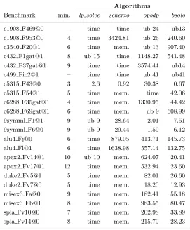
Preliminary results obtained on several instances of the Binate Covering Problem indicate that the proposed techniques are indeed effective and can be significant for specific classes of instances, in par-ticular for instances of covering problems with sets of constraints that are hard to satisfy.
Future research work will naturally include seeking further simpli-fication of the clauses created for each type of conflict, and generalizing the bsoloalgorithm to other boolean optimization problems.
References
1. P. Barth. A Davis-Putnam Enumeration Algorithm for Linear Pseudo-Boolean Optimization. Technical Report MPI-I-95-2-003, Max Plank Institute for Computer Science, 1995.
Table III. Algorithm comparison
Algorithms
Benchmark min. lp solve scherzo opbdp bsolo
c1908 F469@0 – time time ub 24 ub13 c1908 F953@0 4 time 3424.81 ub 26 240.60 c3540 F20@1 6 time mem. ub 13 907.40 c432 F1gat@1 8 ub 15 time 1148.27 541.48 c432 F37gat@1 9 time time 3574.44 ub14 c499 Fic2@1 – time time ub 41 ub41
c5315 F43@0 3 2.6 0.92 30.38 0.67
c5315 F54@1 5 time mem. time 42.06 c6288 F35gat@1 4 time mem. 1330.95 44.42 c6288 F69gat@1 6 time mem. ub 9 608.99 9symml F1@1 9 ub 9 28.64 2.01 7.51 9symml F6@0 9 ub 9 29.44 1.59 6.12 alu4 Fj@0 6 time 879.05 413.71 145.73 alu4 Fl@1 6 time 1638.98 557.14 132.75 apex2 Fv14@1 10 ub 10 mem. 624.07 20.41 apex2 Fv17@1 12 time mem. 532.94 23.60 duke2 Fv5@1 5 time mem. 82.01 26.60 duke2 Fv7@0 5 time mem. 18.20 12.93 misex3 Fa@0 9 time mem. 182.41 55.18 misex3 Fb@1 8 time mem. 983.55 80.47 spla Fv10@0 7 time mem. 202.98 33.89 spla Fv14@0 8 time mem. 215.79 28.23
3. M. S. Bazaraa, J. J. Jarvis and H. D. Sherali Linear Programming and Network Flows. 2nd Ed., John Wiley & Sons, 1989.
4. O. Coudert. Two-Level Logic Minimization, An Overview. Integration, The VLSI Journal, vol. 17(2):677–691, October 1993.
5. O. Coudert. On Solving Covering Problems. InProceedings of the ACM/IEEE Design Automation Conference, June 1996.
6. O. Coudert and J. C. Madre. New Ideas for Solving Covering Problems. In
Proceedings of the ACM/IEEE Design Automation Conference, June 1995. 7. M. Davis and H. Putnam. A Computing Procedure for Quantification Theory.
Journal of the Association for Computing Machinery, vol. 7:201–215, 1960. 8. P. F. Flores, H. C. Neto, and J. P. Marques Silva. An exact solution to the
minimum-size test pattern problem. InProceedings of the IEEE International Conference on Computer Design, pages 510–515, October 1998.
9. J. Gimpel. A Reduction Technique for Prime Implicant Tables. IEEE Transactions on Electronic Computers, vol. EC-14:535–541, August 1965. 10. E. Goldberg, L. Carloni, T. Villa, R. K. Brayton, and A. L.
to unate covering. InProceedings of the ACM/IEEE International Conference on Computer-Aided Design, 1997.
11. G. Hachtel and F. Somenzi. Logic Synthesis and Verification Algorithms. Kluwer Academic Pub., 1996.
12. S. Liao and S. Devadas. Solving Covering Problems Using LPR-Based Lower Bounds. In Proceedings of the ACM/IEEE Design Automation Conference, 1997.
13. M. R. C. M. Berkelaar UNIX Manual Page of lp-solve. In Eindhoven University of Technology, Design Automation Section, ftp://ftp.es.ele.tue.nl/pub/lp solve, 1992.
14. V. M. Manquinho, P. F. Flores, J. P. Marques Silva, and A. L. Oliveira. Prime implicant computation using satisfiability algorithms. In Proceedings of the IEEE International Conference on Tools with Artificial Intelligence, pages 232– 239, November 1997.
15. D. De Micheli. Synthesis and Optimization of Digital Circuits. McGraw-Hill, 1994.
16. G. L. Nemhauser and L. Wolsey. Integer and Combinatorial Optimization. John Wiley & Sons, 1988.
17. J. P. Marques Silva and K. ˜A. Sakallah. GRASP: A new search algorithm for satisfiability. In Proceedings of the ACM/IEEE International Conference on Computer-Aided Design, pages 220–227, November 1996.
18. C. Pizzuti Computing Prime Implicants by Integer Programming. In Proceed-ings of the IEEE International Conference on Tools with Artificial Intelligence, pages 332–336, November 1996.
19. S. J. Russell and P. Norvig Artificial Intelligence: A Modern Approach. Prentice-Hall, 1994.
20. T. Villa, T. Kam, R. K. Brayton, and A. L. Sangiovanni-Vincentelli. Explicit and Implicit Algorithms for Binate Covering Problems.IEEE Transactions on Computer Aided Design, vol. 16(7):677–691, July 1997.
21. S. Yang. Logic Synthesis and Optimization Benchmarks User Guide. Micro-electronics Center of North Carolina, January 1991.
22. H. Zhang. SATO: An efficient propositional prover. In Proceedings of the International Conference on Automated Deduction, pages 272–275, July 1997.
Authors’ Vitae
Vasco Manquinho
Jo˜ao Marques-Silva