On Automated Model-Based Extraction and Analysis of Gait
David K Wagg and Mark S Nixon
School of Electronics and Computer Science, University of Southampton, SO17 1BJ, UK
dkw02r | [email protected]
Abstract
We develop a new model-based extraction process guided by biomechanical analysis for walking people, and analyse its data for recognition capability. Hierarchies of shape and motion yield relatively modest computational demands, while anatomical data is used to generate shape models consistent with normal human body proportions. Mean gait data is used to create prototype gait motion models, which are adapted to fit individual subjects.
Our approach is evaluated on a large gait database, comprising 4824 sequences from 115 subjects, demonstrating gait extraction and description capability in laboratory and real-world capture conditions. Recognition capability is illustrated by an 84% CCR in laboratory conditions, which is reduced for real-world (outdoor) data. Preliminary results from a statistical analysis of the extracted gait parameters, suggest that recognition capability is primarily gained from cadence and from static shape parameters, although gait is the cue by which these are derived.
1. Introduction
Gait may be defined as the individual pattern of movement produced as a person walks. When all gait parameters are considered, this pattern is sufficiently unique for each individual to be employed as a biometric [1, 2]. Gait analysis is usable from a distance and does not require the subject to be aware of or cooperate with its use, making it particularly valuable in surveillance, or other applications where non-contact operation is required [3].
Most existing approaches to gait analysis are data-driven, typically using a person’s silhouette or features derived from it as the basis for recognition [4, 5, 6, 7, 8, 9, 10]. This methodology has many advantages, chiefly of speed and simplicity, but has the disadvantage that silhouette dynamics are only indirectly linked to gait dynamics. It is difficult to infer the importance of different gait components from silhouette dynamics, and it is unclear how a silhouette-based feature set could be normalised for noise, variations in clothing and other dependencies.
Model-based approaches incorporate knowledge of the shape and dynamics of human gait into the extraction process [11, 12, 13, 14]. Using a model ensures that only image data corresponding to allowable human shape and motion is extracted, reducing the effects of noise. This also means that gait dynamics are extracted directly by determining joint positions, rather than inferring dynamics from other measures. An indirect benefit is that a parametric gait model enables us to measure the relative importance of different components of gait in the recognition process.
However, the use of a parametric model introduces its own problems. Success in recognition is dependent on the gait signature being sufficiently complex to incorporate individual variation across the subject population, so that a given subject can be distinguished from all the other subjects under test. As gait is dependent on a large number of parameters (such as joint angles and body segment sizes), this requirement leads to complex models with many free parameters. Finding the best fit model for the subject thereby necessitates searching a high-dimensional parameter space, with correspondingly high computational requirements.
Early approaches have dealt with this problem by severely limiting model complexity, improving speed at the cost of extraction accuracy. Later solutions have often applied numerical optimisation and search strategies, to strike a balance between speed, reliability and accuracy. Finding the correct balance is, however, difficult. To reduce the computational requirements of a model-based approach, we employ a model hierarchy composed of shape and motion components. We assume that a single subject is present in the scene, moving at an approximately constant speed fronto-parallel to the camera, against a cluttered background.
2. Gait Signature Extraction
Fig. 1b demonstrates how the edges of an object at each frame will accumulate to a single area at the correct accumulation velocity, producing an average global view of the object.2.1. Bulk Motion and Shape Estimation
For subjects walking fronto-parallel to a static camera, motion is dominated by velocity in the horizontal plane. This motivates a hierarchical decimation of motion, determining initially horizontal motion and, subsequently, articulated motion components.
Each moving object in the scene will appear as a peak in a plot of maximal accumulation intensity against velocity. If the subject is the most significant moving object in the scene (in terms of edge strength and visibility), their velocity can be inferred by selecting the highest peak in this plot. However, for uncontrolled capture conditions this assumption may not hold true. Consequently, this measure is used as a filtering step, to remove velocities from consideration that do not appear significant or consistent. Currently a threshold is set at the mean of the peak accumulation intensities, typically removing around 75% of candidate velocities.
Image data is pre-processed (Fig. 1a) using a Gaussian averaging filter for noise suppression, followed by Sobel edge detection and background subtraction (the background is computed as the temporal median of neighbouring frames). This removes all static objects, leaving only edges belonging to moving objects.
To determine the bulk motion of the subject in the horizontal plane, we employ a motion-compensated temporal accumulation algorithm [15]. This is effectively the same global temporal accumulation step as in the velocity Hough transform [16], but without shape specificity:
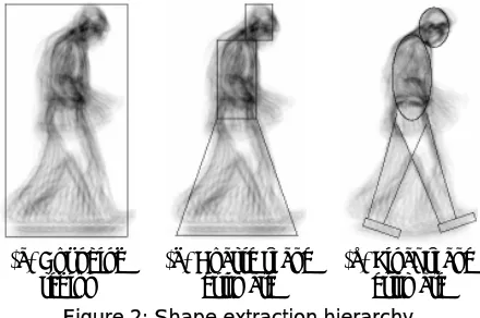
The remaining accumulations are evaluated using a combination of region-based and boundary-based template matching, finding the accumulation best matching a coarse person-shaped template. This template is constructed from mean anatomical data [17] scaled to the subject’s apparent height (Fig. 2b).
( )
∑
−=
−
− + = 1
0
, 2 ,
N
t
t t
v t j dy
N v i E j
i
A (1)
Where Av is the accumulation for velocity v (in pixels per frame), Et is the edge strength image at frame t, i and j are coordinate indices, N is the number of frames in the gait sequence and dyt is the y-displacement of the subject from their centre of oscillation at frame t. This final quantity is initially unknown and set to zero. However, after estimating articulated motion (Sect. 2.2), this information can be used to obtain an improved temporal accumulation.
(a) Bounding
region (b) Coarse shape estimate (c) Final shape estimate Noting that Eqn. 1 simply shifts and accumulates each
[image:2.612.326.546.336.482.2]frame, we can improve computational efficiency by first run-length encoding the input data. This representation is shift-invariant and, as runs of zero magnitude edge strength can simply be discarded, the order of the algorithm is reduced to O(V⋅E⋅N); where V is the number of possible velocities, E is the mean number of edge points in each frame and N is the number of frames in the gait sequence.
Figure 2: Shape extraction hierarchy
By this process we derive an initial estimate of the subject’s starting position, velocity and size, sufficient for estimation of their gait period (Sect. 2.2). This information may in turn be used to predict motion in the vertical plane using Eqn. 6, which permits a re-estimation of the subject’s temporal accumulation using Eqn. 1.
(a) Section of pre-processed
image data (b) Global temporal accumulation
To this accumulation we can apply a more accurate model of the subject’s bulk shape (Fig. 2c), using an ellipse for the torso and for the head. Four line segments are used to model each leg and a rectangle for each foot; parameters describing leg segment lengths and widths are initially set to fixed proportions of the subject’s height. The parameters describing the head and torso are determined separately by template matching within the locality of the initial segmentation, constrained by mean anatomical proportions:
B I y x
S x y r r T T
[image:2.612.65.276.545.699.2]T ( , , , )= +2 (2)
Where TS is the score for a template with position (x,y)
and radii (rx,ry), TI is the sum accumulation intensity within the template region and TB is the sum accumulation intensity on the template boundary. Note that TI is an expansion term favouring larger ellipses, and TB is effectively a stopping criterion. The score weighting was determined empirically and should not be considered optimal, though it performs sufficiently well here.
Gait frequency is determined by finding the frequency and phase that minimises the error function given by Eqn. 4. This minimisation can be performed very quickly for the typical ranges of frequency and phase expected for a walking person.
(
)
(
)
∑
− = + + − = 1 0 2 11 2 sin N t j i s ts R A wt
X
φ
π
(4)Where Xs is the energy function to be minimised, N is the number of frames, Rt is the normalised signal magnitude at frame t, As is the sinusoid amplitude (a fixed ratio of the signal mean magnitude), wi and φj are the proposed gait frequency and phase. Note that the dominant signal frequency is twice that of gait frequency, and a small constant phase shift is required to align the two sinusoids. Although all shape dynamics are lost in the temporal
accumulation process, it is still possible to estimate the amplitude of hip rotation, which may be used to aid articulated motion estimation.
2.2. Articulated Motion Estimation
The motion of the leg during normal gait is periodic, and may be approximately modelled by a single sinusoid [11]. In general, motion periodicity is determined by measuring some quantity related to shape over time and analysing this signal for periodicity. Cutler et al. [18] present a general method for periodicity detection by measuring silhouette self-similarity over time, using autocorrelation-based analysis to extract the gait period. However, this method has relatively high computational demands, particularly for long gait sequences. Other common methods involve analysing periodicity in silhouette width or height [4, 5], which result in far lower computational requirements. We employ a similar strategy, measuring instead sum edge strength within the outer region of the subject’s legs over time (Fig. 3). This region is computed as a fixed ratio of the subject’s height, assuming mean stride length and leg proportions.
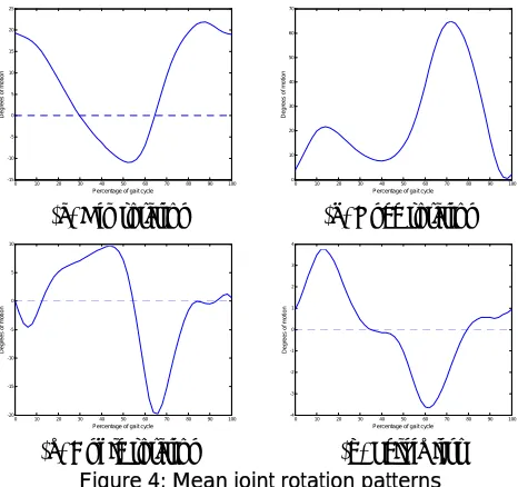
We use data collected from clinical gait studies [2, 19] to build prototypical models for hip, knee, ankle and pelvis rotation. Fig. 4 shows these mean rotation models for a single gait cycle, from right strike to right heel-strike.
0 10 20 30 40 50 60 70 80 90 100 -15 -10 -5 0 5 10 15 20 25
Percentage of gait cycle
D e gr ee s of m o ti on
(a) Hip rotation
0 10 20 30 40 50 60 70 80 90 100 0 10 20 30 40 50 60 70
Percentage of gait cycle
D e gr ee s of m o ti on
(b) Knee rotation
0 10 20 30 40 50 60 70 80 90 100 -20 -15 -10 -5 0 5 10
Percentage of gait cycle
D e gr ee s of m o ti on
(c) Ankle rotation
0 10 20 30 40 50 60 70 80 90 100 -4 -3 -2 -1 0 1 2 3 4
Percentage of gait cycle
D e gr ee s of m o ti on
[image:3.612.318.551.311.530.2](d) Pelvic list
Figure 4: Mean joint rotation patterns
[image:3.612.70.284.441.592.2]Movement of the pelvis includes both axial rotation and list (resulting in horizontal and vertical oscillation respectively in the sagittal plane), but pelvic axial rotation is simple enough to be modelled by a single sinusoid, with a minimal degree of error:
Figure 3: Gait period estimation using within-region edge strength measurements
(
h)
p
p t A wt φ
θ ( )= cos + (5) The measured signal is normalised to remove major
variations due to noise and occlusions [15]: Where θp is pelvic axial rotation, Ap is the amplitude of rotation (approximately 5° for normal gait), w is the gait frequency and φh is the starting gait phase. Although the magnitude of pelvic rotation is small, accounting for this source of variation in hip joint position can significantly reduce errors in the estimation of hip joint rotation. ) | ) ( | ( ) ( M p M p M p M R − −
= (3)
Where R is the normalised signal, M is the measured signal and p(x) denotes the best 2nd-order polynomial fit to
using TCB spline interpolation [20]. This yields an initial estimate of the subject’s limb motion, providing a good basis for adaptation (Sect. 2.3).
The vertical oscillation of the subject’s upper body is also modelled by a single sinusoid, with parameters proportional to the subject’s height and gait motion:
(
8)
2
sin +φ +π
= y h
t A wt
dy (6)
Where dyt is the y-displacement of the centre of the torso at frame t (as used in Eqn. 1), Ay is the amplitude of oscillation, w is the gait frequency and φh is the starting gait phase.
2.3. Gait Motion Model Adaptation
The use of mean gait models allows us to extract approximate joint positions for the subject, but this is not sufficient for recognition purposes. The estimation process assumes average gait motion, implying no individuality. To capture individual variation, adaptation of our mean leg motion models (Fig. 4) is required.
However, before we can match our leg model to image data, it is necessary to improve our estimate of the shape of the subject’s leg. Our initial estimates of leg width at the hip, knee and ankle may not be appropriate for certain types of clothing (baggy trousers, shorts or skirts for example). An improved estimate is obtained by computing a line Hough transform for each frame within the upper and lower leg regions (above and below knee level). Within each Hough space we find the pair of accumulation peaks satisfying constraints on the expected rotation of the leg and the distance between the two lines (leg width), yielding an estimate of leg shape for that frame. Final estimates of leg width are computed as the mean of the best parameters from each frame, weighted by accumulation intensity:
∑
∑
−= −
=
= 1
0 1
0
N
t t N
t t t
m pw p
w (7)
Where wm is the mean width of the leg (at the hip, knee or ankle) over N frames, and wt and pt are the estimated leg width and the peak accumulation intensity respectively at frame t. This process yields estimates of width at the hip and ankle, and two at the knee (from upper leg and lower leg estimation), allowing for discontinuity in leg width at the knee (caused by a skirt or shorts).
For the purpose of adaptation, the rotation models are sampled at 15 points over a single gait cycle. This choice is motivated by a study [21] indicating that the majority of gait information is contained below 5Hz, implying a minimum sampling rate of 10Hz. For a typical gait cycle duration of 1 second, 15 samples per cycle is equivalent to a sampling frequency of 15Hz; this leaves us some room for subjects with long gait cycles.
Adaptation of the joint rotation models is performed via a simple iterative gradient descent procedure with smoothness constraints. The hip and knee models are
adapted jointly for increased accuracy and robustness; ankle rotation is adapted in a subsequent stage. The left and right legs are assumed to move identically at a constant phase difference of π radians, so the same rotation model can be applied to both legs. This additional averaging reduces difficulties caused by self-occlusion of the subject’s legs during gait, contributing to a more robust extraction.
Rotation models are adapted by adding or subtracting a Gaussian function to each model sample. The use of a Gaussian adaptation function enforces the smoothness of motion constraint; any change in sample magnitude proportionally affects neighbouring samples:
0 2 4 6 8 10 12 14
-0.2 -0.1 0 0.1 0.2 0.3 0.4 0.5
Sample number
R
o
ta
ti
o
n
(
radi
ans
) Figure 5: Joint
rotation model adaptation by Gaussian addition
Eqn. 8 describes the model update function applied to each model time instance:
] [ ] [ ]
['n =θ n +δ⋅Gn
θ ,
0
≤
n
<
N
, (8)
} 1 , 0 , 1
{ −
∈
δ
Where θ[n] and θ’[n] are the original and updated joint rotation models respectively (hip, knee or ankle), n is a time index, N is the number of frames and G[n] is a Gaussian function of fixed (small) amplitude and width, centred about the current sample and δ determines the sign of the function. The choice of δ at each sample instance is determined by template matching the leg shape model (Fig. 2c) against edge data over the whole gait sequence. The hip and knee joint rotations are adapted jointly, yielding the evaluation function:
(
)
∑
−=
= 1
0
), ' , ' ( )
, (
N
t
t k h t k
h match M E
S δ δ θ θ (9)
Where S denotes the score for the set (δh, δk), Mt is the shape model at frame t given by the rotation models (θ’h,
θ’k) and Et is the edge intensity image at frame t. The function match denotes the template matching operation summing the edge strength coinciding with the leg shape model over all N frames in the gait sequence.
[image:4.612.323.549.235.341.2]3. Results
Prior to measuring recognition performance, analysis of variance (ANOVA) was applied to the feature vectors extracted for each sequence, aiming to identify which features best distinguish the subjects under test. The ANOVA f-statistic is an approximate measure of discriminatory capability; a high number indicates low intra-subject variance and high inter-subject variance. The performance of the gait extraction process was [image:5.612.319.551.183.262.2]evaluated on the Southampton HiD database [22]. Each subject was filmed from a fronto-parallel viewpoint, in controlled laboratory conditions and in uncontrolled outdoor conditions. The database is encoded in Digital Video (DV) format at a resolution of 720x576 pixels, recorded at a rate of 25 frames per second with approximately 90 frames per gait sequence.
Table 1: ANOVA analysis, indoor dataset
Rank Feature F-statistic 1 Lower knee width 249.54
2 Ankle width 207.76
3 Gait frequency 168.12
4 Upper knee width 86.28
5 Head x-displacement 77.93
Table 2: ANOVA analysis, outdoor dataset
Rank Feature F-statistic 1 Lower knee width 72.26
2 Gait frequency 58.50
3 Ankle width 56.45
4 Upper knee width 48.79
5 Head x-displacement 34.92
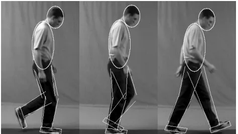
Figure 6: Example model extraction (indoor data)
This analysis suggests that the majority of the system’s discriminatory capability is derived from gait frequency (cadence) and from some static shape parameters (head displacement refers to the displacement of the subject’s head centre from their torso centre). Of course, these shape parameters will be highly dependent on clothing, which limits the utility of performing recognition solely on the basis of these parameters. However, these results may in part explain why approaches using primarily static parameters [7] or cadence [4] can attain good recognition capability with relatively few parameters.
Figure 7: Example model extraction (outdoor data)
There is a significant reduction in discriminatory capability in features extracted from the outdoor dataset compared to those from the indoor dataset, resulting from lower extraction accuracy on this more difficult dataset. Despite the reduction, there is still a strong case for recognition potential using this data.
Recognition performance is evaluated on a large database of 115 subjects, totalling 2163 indoor and 2661 outdoor gait sequences. A 2.4GHz Pentium 4-based PC was used for all testing, requiring approximately 15 hours in pre-processing and 15 hours in gait extraction for the whole database, equivalent to an overall processing rate of around 4 frames per second. This extraction process is fully automated, producing a feature vector for each gait sequence of 63 parameters. 45 of these parameters are the joint rotation model samples for the hip, knee and ankle. The remainder are static parameters describing the subject’s speed, gait frequency and body proportions. The subject’s speed and body segment parameters are divided by the apparent height of the subject to make them size-invariant (the measured size of the subject will vary according to their distance from the camera).
[image:5.612.59.296.200.333.2][3] L Wang, W Hu and T Tan. “Recent Developments in Human Motion Analysis.” Pattern Recognition, 36 (3), pp. 585-601,
2003.
0.3 0.4 0.5 0.6 0.7 0.8 0.9 1.0
1 2 3 4 5 6 7 8 9 10 11 12 13 14 15 16 17 18 19 20
Rank
Ma
tc
h
P
ro
b
a
b
ili
ty
Indoor Dataset Outdoor Dataset
[4] C BenAbdelkader, R Cutler and L Davis. “Stride and Cadence as a Biometric in Automatic Person Identification and Verification.” Proc. FGR, pp. 372-377, 2002.
[5] R T Collins, R Gross and J Shi. “Silhouette-based Human Identification from Body Shape and Gait.” Proc. FGR, pp. 351-356, 2002.
[6] J B Hayfron-Acquah, M S Nixon and J N Carter. “Automatic Gait Recognition by Symmetry Analysis.” Pattern Recognition Letters, 24 (13), pp. 2175-2183.
[7] A Y Johnson and A F Bobick. “A Multi-View Method for Gait Recognition Using Static Body Parameters.” Proc. AVBPA, pp. 301-311, 2001.
[image:6.612.63.294.72.237.2][8] A Kale, N Cuntoor, B Yegnanarayana, A N Rajagopolan and R Chellappa. “Gait Analysis for Human Identification.” Proc. AVBPA, pp. 706-714, 2003.
Figure 8: Cumulative Match Characteristic
Note that the Correct Classification Rate (CCR) is given by the CMC for a rank of one, showing a CCR of approximately 84% on the indoor dataset and 64% on the outdoor dataset.
[9] L Lee and W E L Grimson. “Gait Analysis for Recognition and Classification.” Proc. FGR, pp. 155-162, 2002.
[10] P J Phillips, S Sarkar, I Robledo, P Grother and K Bowyer. “The Gait Identification Challenge Problem: Data Sets and Baseline Algorithm.” Proc. FGR, pp. 137-142, 2002.
4. Conclusions
[11] D Cunado, M S Nixon and J N Carter. “Automatic Extraction and Description of Human Gait Models for Recognition Purposes.” CVIU, 90 (1), pp. 1-41, 2003.We have presented a new fully automated model-based method for gait extraction, based on the hierarchical application of mean shape and motion information and local adaptation. This yields fast and accurate operation even in relatively noisy data, and has proved capable of handling a large database of indoor and outdoor data, generating a parameterised model of an unknown subject suitable for recognition purposes.
[12] D Meyer, J Posl and H Niemann. “Gait Classification with HMMs for Trajectories of Body Parts Extracted by Mixture Densities.” Proc. BMVC, pp. 459-468, 1998.
[13] H Ning, L Wang, W Hu and T Tan. “Articulated Model-Based People Tracking Using Motion Models.” Proc. Int. Conf. on Multimodal Interfaces, 2002.
[14] C Yam, M S Nixon and J N Carter. “On the Relationship of Human Walking and Running: Automatic Person Identification by Gait.” Proc. ICPR, pp. 287-290, 2002. Our statistical analysis suggests that the majority of
recognition potential lies in static shape parameters and cadence, although a more complex parametric model may reveal greater recognition potential in gait dynamics.
[15] D K Wagg and M S Nixon. “Model-Based Gait Enrolment in Real-World Imagery.” Proc. Multimodal User Authentication, pp. 189-195, 2003.
[16] J M Nash, J N Carter and M S Nixon. “Dynamic Feature Extraction via the Velocity Hough Transform.” Pattern Recognition Letters, 18 (10), pp. 1035–1047, 1997.
In the future we intend to investigate the use of more flexible model-based methods, in an effort to resolve the conflict between model complexity and model descriptive
capability. [17] D A Winter. “Biomechanics and Motor Control of Human Movement (2nd Edition).” John Wiley and Sons, 1990. [18] R Cutler and L Davis. “Robust Real-Time Periodic Motion Detection, Analysis, and Applications.” IEEE Trans. PAMI,
22 (8), pp. 781-796, 2000. Acknowledgements
[19] M W Whittle and D Levine. “Three-dimensional Relationships between the Movements of the Pelvis and Lumbar Spine during Normal Gait.” Human Movement Science, 18, pp. 681-692, 1999.
We gratefully acknowledge partial support by the European Research Office of the US Army under Contract No. N68171- 01-C-9002.
[20] D Kochanek and R Bartels. “Interpolating Splines with Local Tension, Continuity and Bias control.” Computer Graphics, 18 (3), pp. 33-41, 1984.
References
[21] C Angeloni, P O Riley and E D Krebs. “Frequency Content of Whole Body Gait Kinematic Data.” IEEE Trans. Rehabilitation Engineering, 2 (1), pp. 40-46, 1994.
[1] M S Nixon, J N Carter, D Cunado, P S Huang and S V Stevenage. “Automatic Gait Recognition.” Biometrics: Personal Identification in Networked Society, Kluwer
Academic Publishing, pp. 231-250, 1999. [22] J D Shutler, M G Grant, M S Nixon and J N Carter. “On a Large Sequence-based Human Gait Database.” Proc. Recent Advances in Soft Computing, pp. 66-71, 2002.