On the Eigenspectrum of the Gram Matrix and the
Generalisation Error of Kernel PCA
John Shawe-Taylor
School of Electronics and Computer Science, University of Southampton
Email:
[email protected]
Christopher K.I. Williams
Division of Informatics, University of Edinburgh
Email:
[email protected]
Nello Cristianini
Department of Statistics, University of California at Davis
Email:
[email protected]
Jaz Kandola
Merrill Lynch Quantitative Analytics Division
2 King Edward Street London EC1A 1HQ
Email:
Jasvinder [email protected]
Abstract— In this paper we analyze the relationships between
the eigenvalues of the m×m Gram matrix K for a kernel κ(·,·) corresponding to a sample x1, . . . ,xm drawn from a densityp(x)and the eigenvalues of the corresponding continuous eigenproblem. We bound the differences between the two spectra and provide a performance bound on kernel PCA showing that we can expect good performance even in very high dimensional feature spaces provided the sample eigenvalues fall sufficiently quickly.
I. INTRODUCTION
Over recent years there has been a considerable amount of in-terest in kernel methods such as Support Vector Machines [1], Gaussian Processes etc in the machine learning area. In these methods the Gram matrix plays an important rˆole. Them×m Gram matrix K has entriesκ(xi,xj),i, j= 1, . . . , m, where
{xi:i = 1, . . . , m} is a given dataset and κ(·,·)is a kernel
function. For Mercer kernels K is symmetric positive semi-definite. We denote its eigenvalues ˆλ1 ≥ ˆλ2. . . ≥ ˆλm ≥ 0
and write its eigendecomposition as K = VΛVˆ 0 where Λˆ
is a diagonal matrix of the eigenvalues and V0 denotes the
transpose of matrix V. The eigenvalues are also referred to as the spectrum of the Gram matrix, while the corresponding columns of V are their eigenvectors.
A number of learning algorithms rely on estimating spectral data on a sample of training points and using this data as input to further analyses. For example in Principal Component Anal-ysis (PCA) the subspace spanned by the firstkeigenvectors is used to give ak dimensional model of the data with minimal residual, hence forming a low dimensional representation of the data for analysis or clustering. Recently the approach has been applied in kernel defined feature spaces in what has become known as kernel-PCA [2]. This representation has also been related to an Information Retrieval algorithm known
as latent semantic indexing, again with kernel defined feature spaces [3].
Furthermore eigenvectors have been used in the HITS [4] and Google’s PageRank [5] algorithms. In both cases the entries in the eigenvector corresponding to the maximal eigenvalue are interpreted as authority weightings for individual articles or web pages.
The use of these techniques raises the question of how reliably these quantities can be estimated from a random sample of data, or phrased differently, how much data is required to obtain an accurate empirical estimate with high confidence. Ng et al. [6] have undertaken a study of the sensitivity of the estimate of the first eigenvector to perturbations of the connection matrix. They have also highlighted the potential instability that can arise when two eigenvalues are very close in value, so that their eigenspaces become very difficult to distinguish empirically.
Other authors have studied the concentration of linear func-tionals of the spectral measure or single eigenvalues of random matrices generated through distributions defined over their entries, see for example Guionnet and Zeitouni [7] and Alon
et al. [8].
performance even in very high dimensional feature spaces provided that the sample eigenvalues fall sufficiently quickly. In this sense the results give a dimension independent bound on the performance of kernel PCA.
The second question that motivated the research reported in this paper is the relation between the eigenvalues of the Gram matrix and those of the underlying process. For a given kernel function and density p(x) on a space X, we can also write down the eigenfunction problem
Z
X
κ(x,y)p(x)φi(x)dx=λiφi(y). (1)
Note that the eigenfunctions are orthonormal with respect to p(x), i.e. Z
X
φi(x)p(x)φj(x)dx=δij.
Let the eigenvalues of the underlying process be ordered so that λ1 ≥ λ2 ≥ . . .. This continuous eigenproblem can be approximated in the following way. Let {xi:i = 1, . . . , m}
be a sample drawn according to p(x). Then
Z
X
κ(x,y)p(x)φi(x)dx' 1
m
m
X
k=1
κ(xk,y)φi(xk) (2)
As pointed out in [9], the standard numerical method (see, e.g., [10], chapter 3) for approximating the eigenfunctions and eigenvalues of equation (1) is to use a numerical approxima-tion such as equaapproxima-tion (2) to estimate the integral, and then plug iny=xj for j= 1, . . . , m to obtain a matrix eigenproblem
m
X
k=1
κ(xk,xj)φi(xk) = ˆλiφi(xj).
Thus we see that µidef=m1λˆi is an obvious estimator for the
ith eigenvalue of the continuous problem. The theory of the numerical solution of eigenvalue problems ([10], Theorem 3.4) shows that for a fixed k,µk will converge toλk in the limit
as m→ ∞.
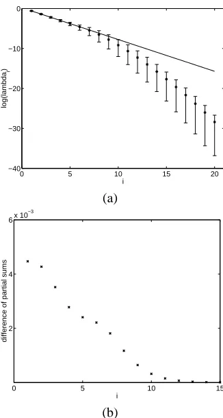
For the case that X is one dimensional andp(x)is Gaussian and κ(x, y) = exp−b(x−y)2 (the RBF kernel with length-scaleb−1/2), there are analytic results for the eigenvalues and eigenfunctions of equation (1) as given in section 4 of [11]. To compare the process eigenvalues with empirical eigenvalues 1000 samples of size m = 100 were used, with parameters b= 3andp(x)∼ N(0,1/4). The 1000 repetitions were used to characterize the variability of the empirical eigenvalues. For this case we can therefore compare the values of µi with the
corresponding λi, as shown in Figure 1(a). Figure 1(b) plots
the difference between the average (over 1000 samples) of the partial sum of the firstiempirical eigenvalues against the same partial sum of the process eigenvalues. These two plots show that for i= 1the average empirical eigenvalue overestimates λ1, but that for i >1 the converse is true. Figure 1(b) also shows that the empirical partial sum initially overestimates the process partial sum, but that this gradually declines. One of the results of this paper will be bounds on the degree of overestimation for these partial sums in a fully general setting.
0 5 10 15 20
−40 −30 −20 −10 0
i
log(lambda
i
)
(a)
0 5 10 15
2 4 6x 10
−3
i
difference of partial sums
[image:2.612.357.520.51.356.2](b)
Fig. 1. (a) A plot of the log eigenvalue against the index of the eigenvalue. The straight line is the theoretical relationship. The centre point (marked with a star) in the error bar is the log of the average value ofµk. The upper and lower ends of the error bars are the 97.5% and 2.5% centiles of oflog(µk) respectively taken over 1000 repetitions. (b) A plot of the difference between the average ofPij=1µjandPij=1λjagainsti.
Koltchinskii and Gine [12] discuss a number of results in-cluding rates of convergence of the µ-spectrum to the λ-spectrum. The measure they use compares the whole spectrum rather than individual eigenvalues or subsets of eigenvalues. They also do not deal with the estimation problem for PCA residuals.
Johnstone [13] studies the distribution of the largest eigenvalue of the Gram matrix of a set of vectors whose components are independent Gaussians, though his is also an asymptotic analysis as the dimension of the feature space and the number of vectors tends to infinity at a fixed ratio greater than 1.
In an earlier version of this paper, [14] discussed the con-centration of spectral properties of Gram matrices and of the residuals of fixed projections. However, these results gave deviation bounds on the sampling variability ofµiwith respect
to E[µi], but did not address the relationship of µi to λi or
the estimation problem of the residual of PCA on new data.
In order to state our main results consider a general probability spaceX and a measurable feature mapping ψ
ψ:x∈ X 7−→ψ(x)∈F
that the support of this distribution is bounded in a ball of radiusR inF. We draw an i.i.d. sampleS of mpoints
S= (x1, . . . ,xm)
from X according to p and form the Gram matrix K(S) of their projections intoF
K(S)ij=hψ(xi),ψ(xj)i.
We refer to the composition of the inner product with the projections as the kernel function κ:
κ(x,z) =hψ(x),ψ(z)i,
and similarly to the matrix K(S) as the kernel matrix. It is often convenient to specify the kernelκand define the feature space implicitly by this choice. Such a feature space will exist provided the kernel is symmetric and has the property that all finite kernel matrices are positive semi-definite (see [15] for details). We refer to the eigenvalues λˆ1(S) ≥ ˆλ2(S) ≥
· · · ≥ˆλm(S)of K(S) as the empirical eigenvalues dropping
the dependency onS if this is clear from the context. There is a corresponding self-adjoint operator in the inner product space L2
p(X) defined by
K(f)(x) =
Z
X
f(x0)κ(x,x0)dp(x0).
We refer to the eigenvalues of this operator as the process eigenvalues and denote them byλ1≥λ2≥ · · · ≥λi≥ · · ·.
Given a sequence of numbers ν1≥ν2≥ · · · ≥νm, wherem
may be infinity, we use the notations
ν>k= m
X
i=k+1
νi and ν≤k= k
X
i=1 νi
to denote the tail and initial sums respectively.
We must introduce a further definition before quoting the main results of the paper. This is concerned with the procedure known as Principal Components Analysis that projects multi-dimensional data in the feature spaceF onto the subspaceVˆk
spanned by the first keigenvectors of the correlation matrix
C(S) = 1 m
m
X
i=1
ψ(xi)ψ(xi)0.
Note that we do not restrict the space F to be finite dimen-sional. However, for any finite set of points x1, . . . ,xm, the
feature vectors ψ(x1), . . . ,ψ(xm) span a finite dimensional
subspace of F. Hence, by choosing a basis that spans this subspace and extending to a basis of the whole space, the cor-relation matrix C(S)becomes effectively finite dimensional. We denote projection onto a subspace V by PV(ψ(x)). We
denote the projection onto the orthogonal complement of V by PV⊥(ψ(x)). If V is a one dimensional subspace withv a non-zero element ofV, we will also writePv in place ofPV.
The norm of the orthogonal projection is also referred to as the residual since it corresponds to the distance between the original point and its projection.
We can now state the three main results of this paper. The first is concerned with the residual projections and the sum of the last eigenvalues.
Theorem 1: If we perform PCA in the feature space defined
by a kernel κ(x,z) then with probability greater than1−δ over random m-samples S, for all1≤k≤m, if we project new data onto the space Vˆk, the expected squared residual is
bounded by
λ>k ≤ EhkP⊥
ˆ
Vk(ψ(x))k 2i
≤ min
1≤`≤k
1
mλˆ
>`(S) +1 +
√
`
√
m
v u u
t2
m
m
X
i=1
κ(xi,xi)2
+R2
s
18 mln
µ
2m δ
where the support of the distribution is in a ball of radiusRin the feature space andλi andλˆi are the process and empirical
eigenvalues respectively.
The theorem states that when projecting into the empirical eigen-subspace spanned by the first k eigenvectors the ex-pected squared residual of a randomly drawn test point can with high probability be bounded by a minimum over `≤k of the sum of all but the first ` empirical eigenvalues plus a complexity term that scales likep`/m.
The last term on the right hand side represents the usual dependency on the confidence parameter δ. The expression inside the minimisation involves two terms. The first term is the empirical estimate of the squared residual, which decreases as`increases. The second term is the complexity penalty that grows with increasing`. The expression will reach a minimum at a value `0 approximately where the two expressions have equal values. Hence, the overall bound decreases askincreases up to `0 and remains constant from that point onwards. In practice we expect that the left hand side will continue to decline slowly beyond this point as further dimensions are included. This effect is indeed evident in the experiments reported in the final section.
For applications of kernel PCA the theorem suggests that good capture of the data can be expected provided the empirical eigenvalues decay beforep`/mgrows too big. Indeed this can be used as a criterion for deciding whether subspace projection is justified based on the available training data.
The second theorem considers the sum of the firstk eigenval-ues and the projections into the space spanned by the firstk eigenvectors.
Theorem 2: If we perform PCA in the feature space defined
eigenvalues is bounded by
λ≤k ≥ EhkP
ˆ
Vk(ψ(x))k 2i
≥ max
1≤`≤k
1
mˆλ
≤`(S)−1 +
√
`
√
m
v u u
t2
m
m
X
i=1
κ(xi,xi)2
−R2
s
19 mln
µ
2(m+ 1) δ
where the support of the distribution is in a ball of radiusRin the feature space and λi andˆλi are the process and empirical
eigenvalues respectively.
This result is perhaps more interesting from the perspective of the relation between process and empirical eigenvalues. In particular, it implies a good fit between the partial sums of the largest eigenvalues with indicesk for whichpk/mis small. The final result concerns the projections of data into the 1-dimensional subspace determined by a single eigenvector. In this case it is not possible to obtain a relationship with the process eigenvalues, but the ‘generalisation’ of the empirical projection obeys an even tighter bound than for the larger subspaces.
Theorem 3: If we perform PCA in the feature space defined
by a kernelκ(x,z)then with probability greater than1−δover random m-samples S, for all 1≤k ≤m, if we project new data onto the one dimensional subspaceUˆk spanned by the
k-th eigenvector of C(S), the expected value of the projection of new data satisfies
E h
kPUˆk(ψ(x))k2
i
≥ 1
mλˆk(S)− 2
√
m
v u u
t2
m
m
X
i=1
κ(xi,xi)2
−R2
s
19 mln
µ
2(m+ 1) δ
where the support of the distribution is in a ball of radius R in the feature space and ˆλi are the empirical eigenvalues.
The paper is organised as follows. In Section 2 we give the background results and develop the basic techniques that are required to develop the necessary framework in sections 3 and 4. Section 5 then gives the main results of the paper. We provide experimental verification of the theoretical findings in Section 6, before drawing our conclusions.
II. BACKGROUND ANDTECHNIQUES
We will make use of the following results that can be traced back to the work of Hoeffding [16] and Azuma [17]. We quote versions given by McDiarmid [18]. Results of this type bounding the deviation of a random variable from its expected value are often referred to as concentration inequalities. More advanced results of this type due to Boucheron et al. and Talagrand can be found in [19] and [20].
Theorem A : LetX1, . . . , Xnbe independent random variables
taking values in a set A, and assume that f :An →R, and that there existfi:An−1→Rfor 1≤i≤nsatisfying
sup
x1,...,xn
|f(x1, . . . , xn)−fi(x1, . . . , xi−1, xi+1, . . . , xn)| ≤ci,
then for all² >0,
P{f(X1, . . . , Xn)−Ef(X1, . . . , Xn)> ²} ≤exp
µ
−2²2
Pn
i=1c2i
Theorem B : LetX1, . . . , Xnbe independent random variables
taking values in a set A, and assume that f : An →R, for 1≤i≤n
sup
x1,...,xn,xˆi
|f(x1, . . . , xn)−f(x1, . . . , xi−1,xˆi, xi+1, . . . , xn)| ≤ci,
then for all² >0,
P{f(X1, . . . , Xn)−Ef(X1, . . . , Xn)> ²} ≤exp
µ
−2²2
Pn
i=1c2i
We will also make use of the following theorem characteris-ing the eigenvectors of a self-adjoint completely continuous operator in a Hilbert space. This theorem is usually referred to as the Courant Fischer Weyl theorem in its matrix version. We quote it here in the more general form [21].
Theorem C : [Courant-Fischer-Weyl Minimax Theorem] IfT is
a self-adjoint completely continuous operator on a real Hilbert space, then fork= 1,2, . . . ,
λk(T) = max
dim(V)=k06=vmin∈V
hTv,vi hv,vi
= min
dim(T)=m−k+10max6=v∈T
hTv,vi hv,vi ,
with the extrema achieved by the corresponding eigenvector.
The approach we adopt in the first stage of the analysis is to relate the eigenvalues to the sums of squares of residuals. This is well-known particularly in the case of matrices, following from consideration of the singular value decomposition. We sketch the analysis in the more general operator form since we require this for the process eigenvalues mentioned above. The matrix form is a simple consequence of this general result.
Recall the operator of the form
Kq(f)(x) =
Z
X
f(x0)κ(x,x0)dq(x0),
in the space L2q(X), where q is some distribution over X. Furthermore consider the self-adjoint operator
Cq(·) =
Z
X
hψ(x),·iψ(x)dq(x).
Letv(·), λbe an eigenfunction, eigenvalue pair forKq, that is
Kq(v)(x) =λv(x). Consider the point
u=fq(v) =
Z
X
v(x)ψ(x)dq(x)∈F.
We have
Cq(u) =
Z
X Z
X
κ(x,z)v(z)dq(z)ψ(x)dq(x)
= λ
Z
X
It follows that fq(v), λ is an eigenvector, eigenvalue pair for
Cq. Furthermore, we have
kfq(v)k2 =
Z
X Z
X
v(x)v(z)κ(x,z)dq(x)dq(z)
= λ
Z
X
v(z)2dq(z) =λkvk2q,
in the norm determined by the distribution q. Similarly it is easily verified that if u, λ is an eigenvector, eigenvalue pair for Cq the function
g(u)(·) =hψ(·),ui
is an eigenfunction for Kq with eigenvalueλand
kg(u)k2
q =λkuk2.
Furthermore, we have that
g(fq(v)) =Kq(v) and fq(g(u)) =Cq(u).
It follows from this analysis that the two operators have the same non-zero eigenvalues and there is a 1-1 correspondence between the corresponding eigenvectors, eigenfunctions given by the functions f andg.
If we consider the case where q is the empirical distribution, that is the uniform distribution on a fixed m-sample S, we will see that this analysis forms the basis of kernel PCA. If we chooseqto be the empirical distribution uniform on a fixed sample S, we will denote the operatorsCq andKq byCS and
KS respectively.
If ui, λi are the i-th normalised eigenvector, eigenvalue pair
of the operatorCS in the feature space, this corresponds to the
i-th eigenvector of the correlation matrix
C(S) = 1 m
m
X
i=1
ψ(xi)ψ(xi)0.
The PCA projection of an input xontoui is given by
hψ(x),uii = λi−1/2hψ(x), fq(vi)i
= λ−i 1/2m−1
m
X
j=1
vi(xj)κ(xj,x),
where vi(·), λi are the corresponding eigenfunction,
eigen-value pair of the operator Kq. This equation forms the basis
of kernel PCA, since it implies that the projection of a new point into the space spanned by the i-th eigenvector can be computed as
Pui(ψ(x)) =
λˆ−1/2
i m
X
j=1
vijκ(x,xj)
ui,
where(vij)mj=1,λˆi are thei-th eigenvector and eigenvalue of
the kernel matrix K(S).
Now consider the first eigenvalue of the operatorKq for
gen-eral distributionq. By Theorem C and the above observations
we have
λ1(Kq) = max
06=v∈F
hCq(v),vi
hv,vi
= max 06=v∈F
1
kvk2
Z
X
hψ(x),vi2dq(x) = max
06=v∈FEq
£
kPv(ψ(x))k2
¤
= Eq
£
kψ(x)k2¤− min 06=v∈FEq
£
kP⊥
v(ψ(x))k2
¤
,
where Eq denotes expectation with respect to q, since
kψ(x)k2 = kP
v(ψ(x))k2 +kPv⊥(ψ(x))k2. It follows that the first eigenvector is characterised as the direction for which the expected square of the residual is minimal.
Applying the same line of reasoning to the first equality of Theorem C, delivers the following equality
λk(Kq) = max
dim(V)=k,V⊆F06=vmin∈VEq
£
kPv(ψ(x))k2
¤
. (3)
Notice that this characterisation implies that ifuk is the k-th
eigenvector ofCq, then
λk(Kq) =Eq
£
kPuk(ψ(x))k2
¤
, (4)
which in turn implies that ifVk is the space spanned by the
firstk eigenvectors, then
k
X
i=1
λi(Kq) = Eq
£
kPVk(ψ(x))k 2¤
= Eq
£
kψ(x)k2¤−E
q
£
kP⊥
Vk(ψ(x))k 2¤.(5)
It readily follows by induction over the dimension ofV that we can equally characterise the sum of the first k and last m−k eigenvalues by
k
X
i=1
λi(Kq) = max
dim(V)=kEq
£
kPV(ψ(x))k2
¤
=Eq
£
kψ(x)k2¤− min dim(V)=kEq
£
kPV⊥(ψ(x))k2
¤
, (6)
∞ X
i=k+1
λi(Kq) = Eq
£
kψ(x)k2¤−
k
X
i=1
λi(Kq) (7)
= min dim(V)=kEq
£
kPV⊥(ψ(x))k2
¤
. (8)
Hence, as for the case whenk= 1, the subspace spanned by the first k eigenvalues is characterised as that for which the sum of the squares of the residuals is minimal.
In the case that q is the empirical distribution the results correspond to the matrix form of the residual result, namely that projecting into the eigenspaces corresponding to the largest eigenvalues minimises the average squared residual. If we takeqto be the data generating distributionp, the result describes the fact that the eigenvectors of the operator Cp
characterise the subspaces ofF capturing the largest expected squared residual:
λk(K) = max
dim(V)=k06=vmin∈VE[kPv(ψ(x))k
where V is a linear subspace of the feature space F and we use Eto denote expectation with respect top. Similarly,
k
X
i=1
λi(K) = max
dim(V)=kE
£
kPV(ψ(x))k2
¤
=E£kψ(x)k2¤− min dim(V)=kE
£
kP⊥
V(ψ(x))k2
¤
(10)
∞ X
i=k+1
λi(K) = E
£
kψ(x)k2¤−
k
X
i=1 λi(K)
= min dim(V)=kE
£
kP⊥
V(ψ(x))k2
¤
. (11)
One of the aims of this paper is to elucidate the relationship between these two projections, demonstrating conditions when the quality of the empirical projection matches that of the ‘ideal’ process projection.
We are now in a position to motivate the main results of the paper. We consider the general case of a kernel defined feature space with input space X and probability density p(x). We fix a sample size m and a draw of m examples S = {x1,x2, . . . ,xm} according to p. We fix the feature
space determined by the kernel as given by the mapping
ψ. We can therefore view the eigenvectors of correlation matrices corresponding to finite Gram matrices as lying in this space. Further we fix a feature dimension k. Let Vˆk
be the space spanned by the first k eigenvectors of the correlation matrix corresponding to the sample kernel matrix K(S) with corresponding eigenvalues λˆ1,λˆ2, . . . ,ˆλk, while
Vk is the space spanned by the first k process eigenvectors
with corresponding eigenvalues λ1, λ2, . . . , λk. Similarly, let
ˆ
E[f(x)] denote the expectation with respect to the sample or the empirical mean:
ˆ
E[f(x)] = 1 m
m
X
i=1 f(xi),
while as before E[·] denotes expectation with respect top. We are interested in the relationships between the following quantities:
ˆ
EhkPVˆk(ψ(x))k2
i
= 1 m
m
X
j=1
kPVˆk(ψ(x))k2
= 1 m
k
X
i=1 ˆ λi
E£kPVk(ψ(x))k 2¤ =
k
X
i=1 λi
EhkPVˆk(ψ(x))k2
i
and Eˆ£kPVk(ψ(x))k 2¤.
Bounding the difference between the first and second will relate the process eigenvalues to the sample eigenvalues, while the difference between the first and third will bound the expected performance of the space identified by kernel PCA when used on new data.
Our first two observations follow simply from equation (10),
ˆ
E h
kPVˆk(ψ(x))k2
i
= 1 m
k
X
i=1 ˆ λi≥Eˆ
£
kPVk(ψ(x))k
2¤ (12) and
E£kPVk(ψ(x))k 2¤=
k
X
i=1 λi ≥E
h
kPVˆk(ψ(x))k
2i (13)
Our strategy will be to show that the right hand side of inequality (12) and the left hand side of inequality (13) are close in value making the two inequalities approximately a chain of inequalities. We then bound the difference between the first and last entries in the chain.
First, however, in the next section we will examine averages over random m samples. We will use the notation Em[·] to
denote this type of average though we could equivalently write
Em[·] in the sense that this is simply the expectation with
respect to them-fold product distribution.
III. AVERAGING OVERSAMPLES ANDPOPULATION EIGENVALUES
The sample correlation matrix is C(S) = 1
mXX0 with
eigenvaluesµ1 ≥µ2. . . ≥µd. (Ifx is a zero-mean random
variable then this is also the covariance matrix.) In the notation of the section IIµi= (1/m)ˆλi. The corresponding population
correlation matrix has eigenvalues λ1 ≥ λ2. . . ≥ λd and
eigenvectors u1, . . . ,ud. Again by the observations above
these are the process eigenvalues.
Statisticians have been interested in the sampling distribution of the eigenvalues of C(S) for some time. There are two main approaches to studying this problem, as discussed in section 6 of [22]. In the case thatxhas a multivariate normal distribution, the exact sampling distribution ofµ1, . . . , µd can
be given [23]. Alternatively, the “delta method” can be used, expanding the sample roots about the population roots. For normal populations this has been carried out in [24] (if there are no repeated roots of the population covariance) and [25] (for the general case), and extended in [26] to the non-Gaussian case.
The following proposition describes howEm[µ1]is related to λ1 andEm[µd] is related toλd. It requires no assumption of
Gaussianity.
Proposition A : [Anderson, 1963, pp 145-146] Em[µ1] ≥λ1
andEm[µd]≤λd.
Proof : By the results of the previous section we have
µ1 = max 06=c
m
X
i=1 1
mkPc(xi)k 2
≥ 1
m
m
X
i=1
kPu1(xi)k2= ˆE
£
kPu1(x)k2
¤
.
We now apply the expectation operatorEmto both sides. On
the RHS we get
EmEˆ
£
kPu1(x)k2
¤
=E£kPu1(x)k2
¤
=λ1
by equation (11), which completes the proof. Correspondingly µd is characterized by µd = min06=cEˆ
£
kPc(xi)k2
¤
Interpreting this result, we see thatEm[µ1]overestimates λ1, while Em[µd] underestimatesλd.
Proposition A can be generalized to give the following result where we have also allowed for a kernel defined feature space of dimension NF ≤ ∞.
Proposition 4: Using the above notation, for any k, 1 ≤
k ≤ m, Em[
Pk
i=1µi] ≥
Pk
i=1λi and Em[
Pm
i=k+1µi] ≤
PNF
i=k+1λi.
Proof : Let Vk be the space spanned by the first k process
eigenvectors. Then from the derivations above we have
k
X
i=1
µi= max V: dimV=k
ˆ
E£kPV(ψ(x))k2
¤
≥Eˆ£kPVk(ψ(x))k 2¤.
Again, applying the expectation operator Em to both sides
of this equation and taking equation (11) into account, the first inequality follows. To prove the second we turn max into min,P intoP⊥ and reverse the inequality. Again taking
expectations of both sides proves the second part.
Furthermore, [26] (equation 2) gives the asymptotic relation-ship
Em[µi] =λi+ 1
m
X
j=1,j6=i
λiλj+κij22
λi−λj +O(m
−2), (14)
whereκij22is the bivariate cumulant of order 4 of the marginal distribution of φi andφj (assumed finite).
Remark 5: Proposition 4 also implies that
ENF
"N
F
X
i=1 µi
#
=
NF
X
i=1 λi
if we sample NF points.
We can tighten this relation and obtain another relationship from the trace of the matrix when the support of p satisfies κ(x,x) = C, a constant. For example if the kernel is stationary, this holds since κ(x,x) =κ(x−x) =κ(0) =C. Thus
trace
µ
1 mK
=C=
m
X
i=1 µi.
Also we have for the continuous eigenproblem
R
Xκ(x,x)p(x)dx = C. Using the feature expansion
representation of the kernel κ(x,y) = PNF
i=1λiφi(x)φi(y) and the orthonormality of the eigenfunctions we obtain the following result
m
X
i=1 µi=
NF
X
i=1 λi.
Applying the results obtained in this section, it follows that Em[µ1] will overestimate λ1, and the cumulative sum
Pk
i=1Em[µi] will overestimate
Pk
i=1λi. This behaviour is illustrated in Figure 1(b). At the other end, clearly forNF ≥
k > m,µk≡0 is an underestimate ofλk.
IV. CONCENTRATION OF EIGENVALUES
Section II outlined the relatively well-known perspective that we now apply to obtain the concentration results for the eigenvalues of positive semi-definite matrices. The key to the results is the characterisation in terms of the sums of residuals given in equations (3) and (8).
Theorem 6: Let κ(x,z) be a positive semi-definite kernel
function on a space X, and let p be a probability density function onX. Fix natural numbers m and1 ≤k < m and letS = (x1, . . . ,xm)∈Xm be a sample ofmpoints drawn
according top. Then for all² >0, P
½¯ ¯ ¯
¯m1λˆk(S)−Em
·
1 mˆλk(S)
¸¯ ¯ ¯
¯≥²
¾
≤2 exp
µ
−2²2m R4
,
whereˆλk(S)is thek-th eigenvalue of the matrixK(S)with
entriesK(S)ij =κ(xi,xj)andR2= maxx∈Xκ(x,x).
Proof : The result follows from an application of Theorem A
provided
sup
S
¯ ¯ ¯
¯m1λˆk(S)− 1
mˆλk(S\ {xi})
¯ ¯ ¯
¯≤R2/m.
Let Sˆ = S \ {xi} and let V (Vˆ) be the k dimensional
subspace spanned by the first k eigenvectors of CS (CSˆ). Let κ correspond to the feature mappingψ. Using m times equation (3) for the empirical distribution we have
ˆ
λk(S) ≥ min v∈Vˆ
m
X
j=1
kPv(ψ(xj))k2
≥ min
v∈Vˆ
X
j6=i
kPv(ψ(xj))k2= ˆλk( ˆS)
ˆ
λk( ˆS) ≥ min v∈V
X
j6=i
kPv(ψ(xj))k2
≥ min
v∈V m
X
j=1
kPv(ψ(xj))k2−R2= ˆλk(S)−R2.
Surprisingly a very similar result holds when we consider the sum of the lastm−keigenvalues or the first keigenvalues.
Theorem 7: Let κ(x,z) be a positive semi-definite kernel
function on a space X, and let p be a probability density function onX. Fix natural numbers m and1 ≤k < m and letS = (x1, . . . ,xm)∈Xm be a sample ofmpoints drawn
according top. Then for all² >0, P
½¯ ¯ ¯
¯m1λˆ>k(S)−Em
·
1 mˆλ
>k(S)
¸¯ ¯ ¯
¯≥²
¾
≤2 exp
µ
−2²2m R4
,
and
P
½¯¯
¯
¯m1λˆ≤k(S)−Em
·
1 mˆλ
≤k(S)
¸¯¯
¯
¯≥²
¾
≤2 exp
µ
−2²2m R4
,
where λˆ≤k(S) (λˆ>k(S)) is the sum of (all but) the largest
k eigenvalues of the matrix K(S) with entries K(S)ij =
κ(xi,xj)andR2= maxx∈Xκ(x,x).
Proof : The result follows from an application of Theorem A
provided
sup
S
¯ ¯ ¯
¯m1ˆλ>k(S)−m1ˆλ>k(S\ {xi})
¯ ¯ ¯
Let Sˆ = S \ {xi} and let V (Vˆ) be the k dimensional
subspace spanned by the first k eigenvectors of CS (CSˆ). Let κ correspond to the feature mapping ψ. Usingm times equation (8) for the empirical distribution we have
ˆ
λ>k(S) ≤
m
X
j=1
kPV⊥ˆ(ψ(xj))k2≤
X
j6=i
kPV⊥ˆ(ψ(xj))k2+R2
= ˆλ>k( ˆS) +R2 λ>k( ˆS) ≤ X
j6=i
kP⊥
V(ψ(xj))k2
=
m
X
j=1
kPV⊥(ψ(xj))k2− kPV⊥(ψ(xi))k2≤λ>k(S).
A similar derivation proves the second inequality.
Corollary 8: Consider a feature space F defined by a kernel
κ(x,z)in a spaceX with a distribution densityp(x). Further-more let ˆλi, i= 1, . . . , mbe the empirical eigenvalues. With
probability1−δ over the selection of a random sample ofm points drawn according to p(x)
¯ ¯ ¯
¯m1λˆ≤k(S)−Em
·
1 mˆλ
≤k(S)
¸¯¯
¯
¯≤R2
r
1 mln
2 δ Our next result concerns the concentration of the residuals with respect to a fixed subspace.
Theorem 9: Let p be a probability density function on X.
Fix natural numbers m and a subspace V and let S = (x1, . . . ,xm)∈Xmbe a sample ofmpoints drawn according
to a probability density functionp. Then for all² >0, P{|Eˆ£kPV(ψ(x))k2
¤
−E£kPV(ψ(x))k2
¤
| ≥²} ≤
2 exp
µ
−²2m 2R4
.
Proof : Since we have that
Em
h
ˆ
E£kPV(ψ(x))k2
¤i
=E£kPV(ψ(x))k2
¤
,
the result follows from an application of Theorem B provided
sup
S,xˆi
¯ ¯
¯EˆS
£
kPV(ψ(x))k2
¤
−EˆS\{xi}∪{xiˆ} £
kPV(ψ(x))k2¤¯¯¯≤
R2/m.
Clearly the largest change will occur if one of the pointsψ(xi)
and ψ(ˆxi) lies in the subspace V and the other does not. In
this case the change will be at mostR2/m.
We apply the theorem to the subspaceVk spanned by the first
k process eigenvalues to obtain the following corollary.
Corollary 10: Consider a feature spaceF defined by a kernel
κ(x,z) in a space X with a distribution density p(x). Fur-thermore let Vk be the subspace of F spanned by the first k
process eigenvectors. With probability1−δover the selection of a random sample of mpoints drawn according to p(x)
¯ ¯
¯Eˆ£kPVk(ψ(x))k
2¤−E£kP
Vk(ψ(x))k
2¤¯¯¯≤R2
r
1 mln
2 δ The concentration results of this section are very tight. In the notation of the earlier sections they show that with high
probability
ˆ
EhkPVˆk(ψ(x))k2
i
= 1 m
k
X
i=1 ˆ λi≈Em
h
ˆ
EhkPVˆk(ψ(x))k2
ii
= Em
"
1 m
k
X
i=1 ˆ λi
#
and E£kPVk(ψ(x))k 2¤=
k
X
i=1 λi
≈ Eˆ£kPVk(ψ(x))k
2¤, (15)
where we have used Theorem 7 to obtain the first approximate equality and Theorem 9 with V = Vk to obtain the second
approximate equality.
This gives the sought relationship to create an approximate chain of inequalities
ˆ
E h
kPVˆk(ψ(x))k
2i = 1 m
k
X
i=1 ˆ λi≥Eˆ
£
kPVk(ψ(x))k 2¤
≈ E£kPVk(ψ(x))k 2¤=
k
X
i=1 λi
≥ E
h
kPVˆk(ψ(x))k2
i
. (16)
Notice that using Proposition 4 we also obtain the following diagram of approximate relationships
ˆ
EhkPVˆk(ψ(x))k2
i
≥ Eˆ£kPVk(ψ(x))k 2¤
≈ ≈
Em
h
1
m
Pk
i=1λˆi
i
≥ E£kPVk(ψ(x))k2
¤
.
Hence, the approximate chain could have been obtained in two ways. It remains to bound the difference between the first and last entries in this chain. This together with the concentration results of this section will deliver the required bounds on the differences between empirical and process eigenvalues, as well as providing a performance bound on kernel PCA.
V. LEARNING A PROJECTION MATRIX
This section will work up to a proof of the three main results given in the introduction. The key observation that enables the analysis bounding the difference between
ˆ
E h
kPVˆk(ψ(x))k2
i
= 1 m
k
X
i=1 ˆ λi
and E h
kPVˆk(ψ(x))k
2i is that we can view the projection
normkPVˆk(ψ(x))k2 as a linear function of pairs of features from the feature spaceF.
Proposition 11: LetVˆ be the subspace spanned by some fixed
subsetIofkeigenvectors of the kernel matrix. The projection normkPVˆ(ψ(x))k2 is a linear functionfˆin a feature space
ˆ
F for which the kernel function is given by
ˆ
κ(x,z) =κ(x,z)2.
Proof : Let X =UΣV0 be the singular value decomposition
of the sample matrix X in the feature space. The projection norm is then given by
ˆ
f(x) =kPVˆ(ψ(x))k2=ψ(x)0U(I)U(I)0ψ(x), where U(I) is the matrix containing the k columns of U in the set I. Hence we can write
kPVˆ(ψ(x))k2=
NF
X
ij=1
wijψ(x)iψ(x)j= NF
X
ij=1
wijψˆ(x)ij,
where ψˆ is the projection mapping into the feature space Fˆ consisting of all pairs ofFfeatures andwij = (U(I)U(I)0)ij.
The standard polynomial construction gives
ˆ
κ(x,z) = κ(x,z)2=
ÃN
F
X
i=1
ψ(x)iψ(z)i
!2
=
NF
X
i,j=1
ψ(x)iψ(z)iψ(x)jψ(z)j
=
NF
X
i,j=1
(ψ(x)iψ(x)j)(ψ(z)iψ(z)j)
=
D
ˆ
ψ(x),ψˆ(z)
E
ˆ
F.
It remains to show that the norm of the linear function is k. The norm satisfies (note thatk·kF denotes the Frobenius norm
andui the columns ofU)
kfˆk2 =
NF
X
i,j=1 α2
ij =kU(I)U(I)0k2F
=
* X
i∈I
uiu0i,
X
j∈I
uju0j
+
F
= X
i,j∈I
(u0
iuj)2=k
as required.
We are now in a position to apply a learning theory bound where we consider a regression problem for which the target output is the square of the norm of the sample pointkψ(x)k2. We restrict the linear function in the space Fˆ to have norm
√
k. The loss function is then the shortfall between the output of fˆand the squared norm.
The approach we adopt here makes use of the Rademacher variables and the measure is therefore known as the Rademacher complexity. We refer the reader to Ledoux and Talagrand [27] as a core reference, though we will only be using the results and approach described in [28].
Definition 12: Given a sample S = {x1, . . . ,xm} generated
by a distributionDon a setX and a real-valued function class
F with domain X, the empirical Rademacher complexity of
F is the random variable
ˆ
Rm(F) =Eσ
"
sup
f∈F ¯ ¯ ¯ ¯ ¯
2 m
m
X
i=1
σif(xi)
¯ ¯ ¯ ¯ ¯ ¯ ¯ ¯ ¯
¯x1, . . . ,xm #
,
whereσ={σ1, . . . , σm} are independent uniform{−1,+1}
-valued (Rademacher) random variables. The Rademacher
com-plexity ofF is
Rm(F) =ES
h
ˆ Rm(F)
i
=ESσ
"
sup
f∈F ¯ ¯ ¯ ¯ ¯
2 m
m
X
i=1
σif(xi)
¯ ¯ ¯ ¯ ¯ #
.
Note that we denote the input space with Z in the theorem, so that in the case of supervised learning we would haveZ= Y ×X. The following theorem follows closely the proof of Theorem 8 in Bartlett and Mendelson [28], the small changes allow us to obtain slightly tighter bounds for our special case. We omit the details just noting that bounding in terms of the empirical Rademacher complexity follows from one further application of Theorem B.
Theorem D : (Bartlett and Mendelson, 2002) LetFbe a class
of functions mapping fromZ to[0,1]and letS= (zi)mi=1be drawn independently according to a probability distributionD and fix δ ∈(0,1). Then with probability at least 1−δ over samples of length meveryf ∈ F satisfies
ED[f(z)] ≤ Eˆ[f(z)] +Rm(F) +
r
2ln(2/δ) m
≤ Eˆ[f(z)] + ˆRm(F) +
r
18ln(2/δ) m . (17) Given a training set S the class of functions that we will primarily be considering are linear functions with bounded norm
(
x→
m
X
i=1
αiκ(xi,x) :α0Kα≤B2
)
⊆
{x→ hw, φ(x)i: kwk ≤B}=FB,
where φ is the feature mapping corresponding to the kernel κ(·,·). Note that although the choice of functions appears to depend on S, the definition of FB does not depend on the
particular training set. Bartlett and Mendelson [28] bound the empirical Rademacher complexity of this function class.
Theorem E : (Bartlett and Mendelson, 2002) Ifκ:X×X →
R is a kernel, and S = {x1, . . . ,xm} is a sample of points
from X, then the empirical Rademacher complexity of the classFB satisfies
ˆ
Rm(FB)≤2B
m
v u u
tXm
i=1
κ(xi,xi) = 2B
m
p
tr (K)
The final ingredient that will be required to apply the technique are the properties of the Rademacher complexity that allow it to be bounded in terms of large classes. The following standard theorem summarises the properties of the empirical Rademacher complexity that we require.
Theorem F : LetF andHbe classes of real functions. Then
1) If F ⊆ H, thenRˆm(F)≤Rˆm(H).
2) For everyc∈R,Rˆm(cF) =|c|Rˆm(F)
Theorem 13: If we perform PCA on a randomly drawn
train-ing set S of size min the feature space defined by a kernel κ(x,z) and project new data onto the space Vˆ spanned by a subset I of k eigenvectors, with probability greater than 1−δover the generation of the sampleSthe expected squared residual is bounded by
E£kP⊥
ˆ
V (ψ(x))k
2¤ ≤ 1 m
X
i6∈I
ˆ λi(S)
+1 +
√
k
√
m
v u u
t2
m
m
X
i=1
κ(xi,xi)2+R2
s
18 mln
µ
2 δ
,
where the support of the distribution is in a ball of radius R in the feature space.
Proof. As indicated in Proposition 11 we consider the function
class Fˆ√
k with respect to the kernel
ˆ
κ(x,z) =κ(x,z)2,
with corresponding feature mapping ψˆ. Note that the weight vectors considered satisfy the special condition that they are positive semi-definite, that is that
X
ij
wijψˆ(x)ij≥0,
for all x. Furthermore the function corresponds to the norm squared of a projection mapping. We will denote the subset of functions satisfying this condition by P. We augment the corresponding primal weight vectors with one further dimension while augmenting the corresponding input vectors with a feature
kψ(x))k2k−0.25 = κ(x,x)k−0.25=k−0.25pˆκ(x,x) = kψˆ(x))kk−0.25
that is the norm squared in the original feature space divided by the fourth root ofk. We now apply Theorem D to the class
ˆ
F =
n
f`: ( ˆψ(x),kψˆ(x))kk−0.25)
7→ (kψˆ(x))k −f( ˆψ(x)))R−2 |f ∈Fˆ√
k∩ P
o
⊆ R−2Fˆ√0
k+√k,
where we have restricted the inputs to images of points in the input space as indicated. The squared norm of the image of the inputxunder this feature mapping isˆk(x,x)(1 +k−0.5). The theorem is applied to the functionfˆ`wherefˆis the projection
function of Theorem 11. We must first verify that the range of the function class on the restricted inputs is [0,1]. Since we have restricted ourselves to positive semi-definite weight vectors f( ˆψ(x))≥0, so that
f`( ˆψ(x))≤ kψˆ(x))kR−2≤1.
Furthermore, since we have restrictedFˆ to only contain func-tions that correspond to taking the norm squared of projection mappings in the original feature space we have that
f( ˆψ(x))≤ kψˆ(x))k,
so that f`( ˆψ(x)) ≥ 0 as required. We can therefore apply
Theorem 11. First note that for the functionfˆ` the left hand
side of the expression is equal to 1
R2E
£
kPV⊥ˆ(ψ(x))k 2¤,
whereVˆ is the space spanned by thekeigenvectors in the set I. Hence, to obtain the result it remains to evaluate the two expressions on the right hand side of equation (17). The first is a scaling of the empirical squared residual when projecting into the spaceVˆ, that is
1 R2Eˆ
£
kP⊥
ˆ
V(ψ(x))k
2¤= 1 mR2
X
i6∈I
ˆ λi.
The second expression isRˆm( ˆF)which by Theorem F parts
1 and 2 can be bounded by R−2Rˆ
m
µ
ˆ
F√0
k+√k
. Next we
apply Theorem E to obtain
ˆ Rm
µ
ˆ
F√0
k+√k
≤
p
k+√k m
p
tr (K)
=
s
k+√k m
v u u
t2(1 +k−0.5)
m
m
X
i=1
κ(xi,xi)2
=1 +
√
k
√
m
v u u
t2
m
m
X
i=1
κ(xi,xi)2.
Assembling all the components and multiplying through by R2 gives the result.
We can apply the bound m times to obtain a proof of Theorem 1.
Proof of Theorem 1. We apply Theorem 13 taking I =
{1, . . . , k}, fork= 1, . . . , m, in each case replacingδbyδ/m. This ensures that with probability 1−δ the assertion holds for all m applications. The second inequality of Theorem 1 follows from the observation that fork≥`
E h
kP⊥
ˆ
Vk(ψ(x))k
2i≤EhkP⊥
ˆ
V`(ψ(x))k 2i,
while the first inequality follows from the last inequality of equation (16).
A similar argument applies for Theorem 2.
Proof of Theorem 2. We apply Theorem 13 taking I =
{1, . . . , k}, for k = 1, . . . , m, in each case replacing δ by δ/(m+1). This ensures that with probability1−δthe assertion holds for allm applications together with the assertion that
¯ ¯
¯E
h
kψ(x)k2
i
−Eˆ h
kψ(x)k2
i¯ ¯
¯≤R2
r
1 mln
2(m+ 1) δ . This final inequality follows from a straightforward application of McDiarmid’s inequality. The second inequality of Theo-rem 2 follows from the observations above together with the fact that
1 mλˆ
≤k = ˆEhkψ(x)k2i
− 1
mλˆ
>k,
Finally we give the proof of Theorem 3.
Proof of Theorem 3. Consider applying Theorem 13 taking
I={k}, and replacingδbyδ/(m+1). This ensures that with probability 1−δ the assertion holds for all m applications together with the assertion that
¯ ¯
¯Ehkψ(x)k2i−Eˆhkψ(x)k2i¯¯¯≤R2
r
1 mln
2(m+ 1) δ . This final inequality follows from a straightforward application of McDiarmid’s inequality. The inequality of Theorem 3 follows from the observations above together with the fact that
1 m
X
i6=k
ˆ λi= ˆE
h
kψ(x)k2
i
− 1
mλˆk.
VI. EXPERIMENTS
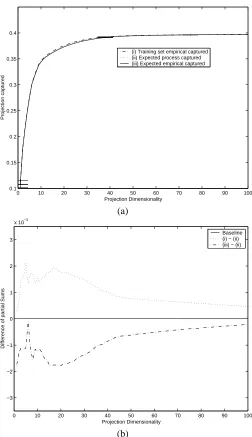
To illustrate the results described in this paper experiments were carried out with the Breast cancer data set [29] which contains 683 data points. This dataset is available from the UCI data repository. A normalised cubic polynomial kernel was chosen,
κN Chxi,xji= hxi,xji
3
p
hxi,xii3hxj,xji3
(18)
from a range of other kernels, based on the empirical obser-vation that the process eigenspectrum did not decay too fast.
We compare three quantities
(i) Eˆ h
kPVˆk(ψ(x))k 2i= 1
m
Pk
i=1λˆi,
(ii) E£kPVk(ψ(x))k
2¤=Pk i=1λi, (iii) E
h
kPVˆk(ψ(x))k 2i.
From inequality (13) we have (ii)≥(iii) and from Proposition 2 we have (i)≥(ii) in the expectationEmwith respect to the
product distribution.
We randomly selected 50% of the data as a ‘training’ set. The process eigenspectrum was obtained by performing an eigen-value decomposition of the kernel matrix constructed from the entire dataset. Similarly the spectrum {ˆλi} was obtained
from an eigendecomposition of the appropriate submatrix. The computation of kPVˆk(ψ(x))k
2 is carried out as explained in
[15].
Figure 2(a) shows the projected squared norm plotted against k for these three quantities. Curves (i) and (iii) have been averaged over 20 random choices of the training set. The error bars give one standard deviation. Notice the close agreement between the curves (i) and (iii), indicating that the subspace identified as optimal for the training set is indeed capturing almost the same amount of information for all data points. The very tight error bars show clearly the very tight concentration of the sums of tail of eigenvalues as predicted by Theorem 7. In order to amplify the information depicted in Figure 2(a), Figure 2(b) plots the differences (i)-(ii) and (iii)-(ii). As expected we see that (i)-(ii)≥0 and (iii)-(ii) ≤0. For larger projection dimensions the theory predicts that the accuracy
0 10 20 30 40 50 60 70 80 90 100
0.1 0.15 0.2 0.25 0.3 0.35 0.4
Projection Dimensionality
Projection captured
(i) Training set empirical captured (ii) Expected process captured (iii) Expected empirical captured
(a)
0 10 20 30 40 50 60 70 80 90 100
−3 −2 −1 0 1 2 3
x 10−3
Difference of partial Sums
Projection Dimensionality
Baseline (i) − (ii) (iii) − (ii)
[image:11.612.313.565.51.488.2](b)
Fig. 2. (a) Plot of the projected squared norm plotted against the projection dimension. The plot shows three curves, (i) expected squared norm for training set when projected into empirical eigenspace averaged over 20 random splits, (ii) expected squared norm for the true process eigenspectrum and (iii) expected squared norm for empirical eigenspace again averaged over 20 random splits. (b) Zooms in on plot (a) by displaying the differences between (i) and (ii) and between (iii) and (ii).
will level off and remain constant and this effect can be observed in Figure 2(b).
VII. CONCLUSIONS
The paper has shown that the eigenvalues of a positive semi-definite matrix generated from a random sample is concen-trated. Furthermore the sum of the last m−k eigenvalues is similarly concentrated as is the residual when the data is projected into a fixed subspace.
dimension of the subspace that captures most of the training data. The results provide a basis for performing PCA or kernel-PCA from a randomly generated sample, as they confirm that the subspace identified by the sample will indeed ‘generalise’ in the sense that it will capture most of the information in a test sample provided that the dimension is small compared to the sample size and that the subspace captures most of the variance in the training data. The result is somewhat counter-intuitive in that the dimension of the feature space does not appear explicitly. The critical quantity is the ratio of the empirical or ‘effective’ dimension of the sample data to the number of examples it comprises.
Experiments are presented that confirm the theoretical predic-tions on a real world data-set for small projection dimensions. For larger projection dimensions the theory predicts that the accuracy will level off and remain constant. In practice there is a slow attenuation with increasing projection dimension. This is not inconsistent with the theory and accords with intuitive expectations.
ACKNOWLEDGEMENTS
CW thanks Matthias Seeger for comments on an earlier version of the paper. We would like to acknowledge the fi-nancial support of EPSRC Grant No. GR/N08575, EU Project KerMIT, No. IST-2000-25341, the Neurocolt working group No. 27150, and the PASCAL Network of Excellence, No. IST-2002-506778.
REFERENCES
[1] N. Cristianini and J. Shawe-Taylor, An Introduction to Support Vector
Machines. Cambridge University Press, 2000.
[2] S. Mika, B. Sch¨olkopf, A. Smola, K.-R. M¨uller, M. Scholz, and G. R¨atsch, “Kernel PCA and de-noising in feature spaces,” in Advances
in Neural Information Processing Systems 11, 1998.
[3] N. Cristianini, H. Lodhi, and J. Shawe-Taylor, “Latent seman-tic kernels for feature selection,” NeuroCOLT Working Group, http://www.neurocolt.org, Tech. Rep. NC-TR-00-080, 2000.
[4] J. Kleinberg, “Authoritative sources in a hyperlinked environment,” in
Proceedings of 9th ACM-SIAM Symposium on Discrete Algorithms,
1998.
[5] S. Brin and L. Page, “The anatomy of a large-scale hypertextual (web) search engine,” in Proceedings of the Seventh International World Wide
Web Conference, 1998.
[6] A. Y. Ng, A. X. Zheng, and M. I. Jordan, “Link analysis, eigenvectors and stability,” in To appear in the Seventeenth International Joint
Conference on Artificial Intelligence (IJCAI-01), 2001.
[7] A. Guionnet and O. Zeitouni, “Concentration of the spectral measure for large matrices,” Electron. Comm. Prob., vol. 5, pp. 119–136, 2000. [8] N. Alon, M. Krivelevich, and V. H. Vu, “On the concentration of eigen-values of random symmetric matrices,” Israel Journal of Mathematics, vol. 131, pp. 259–267, 2002.
[9] C. K. I. Williams and M. Seeger, “The Effect of the Input Density Distribution on Kernel-based Classifiers,” in Proceedings of the
Sev-enteenth International Conference on Machine Learning (ICML 2000),
P. Langley, Ed. Morgan Kaufmann, 2000.
[10] C. T. H. Baker, The numerical treatment of integral equations. Oxford: Clarendon Press, 1977.
[11] H. Zhu, C. K. I. Williams, R. J. Rohwer, and M. Morciniec, “Gaussian regression and optimal finite dimensional linear models,” in Neural
Networks and Machine Learning, C. M. Bishop, Ed. Berlin:
Springer-Verlag, 1998.
[12] V. Koltchinskii and E. Gine, “Random matrix approximation of spectra of integral operators,” Bernoulli, vol. 6(1), pp. 113–167, 2000. [13] I. Johnstone, “On the distribution of the largest
prin-cipal component,” Stanford University, http://www-stat.stanford.edu/ imj/Reports/index.html, Tech. Rep., 2000.
[14] J. Shawe-Taylor, N. Cristianini, and J. Kandola, “On the Concentration of Spectral Properties,” in Advances in Neural Information Processing
Systems 14, T. G. Diettrich, S. Becker, and Z. Ghahramani, Eds. MIT
Press, 2002.
[15] J. Shawe-Taylor and N. Cristianini, Kernel Methods for Pattern Analysis. Cambridge, UK: Cambridge University Press, 2004.
[16] W. Hoeffding, “Probability inequalities for sums of bounded random variables,” J. Amer. Stat. Assoc., vol. 58, pp. 13–30, 1963.
[17] K. Azuma, “Weighted sums of certain dependent random variables,”
Tohoku Math J., vol. 19, pp. 357–367, 1967.
[18] C. McDiarmid, “On the method of bounded differences,” in Surveys in
Combinatorics 1989. Cambridge University Press, 1989, pp. 148–188.
[19] S. Boucheron, G. Lugosi, and P. Massart, “A sharp concentration in-equality with applications,” Random Structures and Algorithms, vol. 16, pp. 277–292, 2000.
[20] M. Talagrand, “New concentration inequalities in product spaces,”
Invent. Math., vol. 126, pp. 505–563, 1996.
[21] H. Voss, “Variational characterization of eigenvalues of nonlinear eigen-problems,” in Proceedings of the International Conference on
Mathe-matical and Computer Modelling in Science and Engineering, 2003, pp.
379–383.
[22] M. L. Eaton and D. E. Tyler, “On Wielandt’s Inequality and Its Application to the Asymptotic Distribution of the Eigenvalues of a Random Symmetric Matrix,” Annals of Statistics, vol. 19(1), pp. 260– 271, 1991.
[23] A. T. James, “The distribution of the latent roots of the covariance matrix,” Annals of Math. Stat., vol. 31, pp. 151–158, 1960.
[24] D. N. Lawley, “Tests of Significance for the Latent Roots of Covariance and Correlation Matrices,” Biometrika, vol. 43(1/2), pp. 128–136, 1956. [25] T. W. Anderson, “Asymptotic Theory for Principal Component Analy-sis,” Annals of Mathematical Statistics, vol. 34(1), pp. 122–148, 1963. [26] C. M. Waternaux, “Asymptotic Distribution of the Sample Roots for a
Nonnormal Population,” Biometrika, vol. 63(3), pp. 639–645, 1976. [27] M. Ledoux and M. Talagrand, Probability in Banach Spaces:
isoperime-try and processes. Springer, 1991.
[28] P. L. Bartlett and S. Mendelson, “Rademacher and gaussian complexi-ties: Risk bounds and structural results,” Journal of Machine Learning
Research, 2002.