Proof Complexity of Propositional Default Logic

This is a repository copy of

Proof Complexity of Propositional Default Logic

.

White Rose Research Online URL for this paper:

http://eprints.whiterose.ac.uk/74805/

Proceedings Paper:

Beyersdorff, O, Meier, A, Mueller, S et al. (2 more authors) (2010) Proof Complexity of

Propositional Default Logic. In: Strichman, O and Szeider, S, (eds.) Theory and

applications of satisfiability testing. SAT 2010, 11-14 July 2010, Edinburgh, UK. Lecture

notes in computer science, 6175 . Springer Verlag , 30 - 43 . ISBN 978-3-642-14185-0

https://doi.org/10.1007/978-3-642-14186-7_5

[email protected] https://eprints.whiterose.ac.uk/

Reuse See Attached Takedown

If you consider content in White Rose Research Online to be in breach of UK law, please notify us by

Proof Complexity of Propositional Default Logic

Olaf Beyersdorff1, Arne Meier2, Sebastian M¨uller3, Michael Thomas2, and Heribert Vollmer2

1 _{Institute of Computer Science, Humboldt University Berlin, Germany}

[email protected]

2 _{Institute of Theoretical Computer Science, Leibniz University Hanover, Germany}

{meier,thomas,vollmer}@thi.uni-hannover.de

3 _{Faculty of Mathematics and Physics, Charles University Prague, Czech Republic}

[email protected]

Abstract. Default logic is one of the most popular and successful formalisms for non-monotonic reasoning. In 2002, Bonatti and Olivetti introduced several sequent calculi for credulous and skeptical reasoning in propositional default logic. In this paper we examine these calculi from a proof-complexity perspec-tive. In particular, we show that the calculus for credulous reasoning obeys almost the same bounds on the proof size as Gentzen’s systemLK. Hence prov-ing lower bounds for credulous reasonprov-ing will be as hard as provprov-ing lower bounds forLK. On the other hand, we show an exponential lower bound to the proof size in Bonatti and Olivetti’s enhanced calculus for skeptical default reasoning.

1 Introduction

Trying to understand the nature of human reasoning has been one of the most fascinating adventures since ancient times. It has long been argued that due to its monotonicity, classical logic is not adequate to express the flexibility of com-monsense reasoning. To overcome this deficiency, a number of formalisms have been introduced (cf. [20]), of which Reiter’s default logic [21] is one of the most popular and widely used systems. Default logic extends the usual logical (first-order or propositional) derivations by patterns for default assumptions. These are of the form “in the absence of contrary information, assume . . . ”. Reiter argued that his logic adequately formalizes human reasoning under theclosed world assumption. Today default logic is widely used in artificial intelligence and computational logic.

The semantics and the complexity of default logic have been intensively studied during the last decades (cf. [7] for a survey). In particular, Gottlob [13] has identified and studied two reasoning tasks for propositional default logic: thecredulous and theskeptical reasoning problem which can be understood as analogues of the classical problems SAT and TAUT. Due to the stronger ex-pressibility of default logic, however, credulous and skeptical reasoning become harder than their classical counterparts—they are complete for the second level

Σp

2 and Π p

2 of the polynomial hierarchy, respectively [13].

⋆_{Research supported in part by DFG grants KO 1053/5-2 and VO 630/6-1, by a grant from}

Less is known about the complexity of proofs in default logic. While there is a rich body of results for propositional proof systems (cf. [17]), proof com-plexity of non-classical logics has only recently attracted more attention, and a number of exciting results have been obtained for modal and intuitionistic logics [14–16]. Starting with Reiter’s work [21], several proof-theoretic methods have been developed for default logic (cf. [1, 11, 18, 19, 22] and [9] for a survey). However, most of these formalisms employ external constraints to model non-monotonic deduction and thus cannot be considered purely axiomatic (cf. [10] for an argument). This was achieved by Bonatti and Olivetti [4] who designed simple and elegant sequent calculi for credulous and skeptical default reasoning. Subsequently, Egly and Tompits [10] extended Bonatti and Olivetti’s calculi to first-order default logic and showed a speed-up of these calculi over classical first-order logic, i.e., they construct sequences of first-order formulae which need long classical proofs but have short derivations using default rules.

In the present paper we investigate the original calculi of Bonatti and Olivetti [4] from a proof-complexity perspective. Apart from some preliminary observations in [4], this comprises, to our knowledge, the first comprehensive study of lengths of proofs in propositional default logic. Our results can be summarized as follows. Bonatti and Olivetti’scredulous default calculus BOcred

obeys almost the same bounds to the proof size as Gentzen’s propositional se-quent calculus LK, i.e., we show that upper bounds to the proof size in both calculi are polynomially related. The same result also holds for the proof length (the number of steps in the system). Thus, proving lower bounds to the size of BOcred will be as hard as proving lower bounds to LK (or, equivalently,

to Frege systems), which constitutes a major challenge in propositional proof complexity [5,17]. This result also has implications for automated theorem prov-ing. Namely, we transfer the non-automatizability result of Bonet, Pitassi, and Raz [6] for Frege systems to default logic: BOcred-proofs cannot be efficiently

generated, unless factoring integers is possible in polynomial time.

While alreadyBOcred appears to be a strong proof system for credulous

de-fault reasoning, admitting very concise proofs, we also exhibit a general method of how to construct a proof system Cred(P) for credulous reasoning from a propositional proof system P. This system Cred(P) bears the same relation to

P with respect to proof size as BOcred does to LK. Thus, choosing for

exam-ple P as extended Frege might lead to stronger proof systems for credulous reasoning.

For skeptical reasoning, the situation is different. Bonatti and Olivetti [4] construct two proof systems for this task. While they already show an exponen-tial lower bound for their first skeptical calculus, we obtain also an exponenexponen-tial lower bound to the proof length in their enhanced skeptical calculus. This lower bound also holds if the enhanced calculus is augmented by further rules such as the cut rule.

calculi. Our main results on the proof complexity of credulous and skeptical default reasoning follow in Sects. 4 and 5, respectively. In Sect. 6, we conclude with a discussion and some open questions.

2 Preliminaries

We assume familiarity with propositional logic and basic notions from com-plexity theory (cf. [17]). ByL we denote the set of all propositional formulae over some fixed standard set of connectives. For T ⊆ L, the set of all logical consequences ofT will be denoted by T h(T).

2.1 Proof Systems

Cook and Reckhow [8] defined the notion of a proof system for an arbitrary languageLas a polynomial-time computable functionf with rangeL. A string

w withf(w) =x is called an f-proof for x∈L. Proof systems for L= TAUT are calledpropositional proof systems. The sequent calculusLK of Gentzen [12] is one of the most important and best studied propositional proof systems. It is well known thatLK and Frege systems mutually p-simulate each other(cf. [17]). There are two measures which are of primary interest in proof complexity. The first is the minimal size of an f-proof for some given element x ∈ L. To make this precise, let sf(x) = min{|w| | f(w) = x} and sf(n) = max{sf(x) | |x| ≤ n}. We say that the proof system f is t-bounded if sf(n) ≤ t(n) for all

n ∈ N_{. If t is a polynomial, then f is called polynomially bounded. Another} interesting parameter of a proof is the length defined as the number of proof steps. This measure only makes sense for proof systems where proofs consist of lines containing formulae or sequents. This is the case for LK and most systems studied in this paper. For such a system f, we let tf(ϕ) = min{k |

f(π) =ϕand π uses ksteps} and tf(n) = max{tf(ϕ) | |ϕ| ≤ n}. Obviously, it

holds that tf(n) ≤sf(n), but the two measures are even polynomially related

for a number of natural systems as extended Frege (cf. [17]).

For sequent calculi one distinguishes between dag-like and tree-like proofs where in the latter notion each derived sequent can be used at most once as a prerequisite of a rule. While forLK these two measures are equivalent [17], we will concentrate here only on the stronger dag-like model.

2.2 Default Logic

Default logic is an extension of classical logic that has been proposed by Reiter [21]. The logic is non-monotonic in the sense that an increase in information may decrease the number of consequences. Adefault theory hW, Di consists of a setW of propositional sentences and a setDofdefaults. A default (rule)δ is an inference rule of the form α:β

γ , whereαandγ are propositional formulae

andβis a set of propositional formulae. Theprerequisite αis also referred to as

p(δ), the formulae inβ are calledjustifications (referred to asj(δ)), andγ is the

terms of a fixed-point equation [21], but we use the following characterization as a starting definition:

Theorem 1 (Reiter [21]). Let E ⊆ L be a set of formulae and hW, Di be a default theory. Furthermore let E0 =W,and

Ei+1=T h(Ei)∪ {c(δ)|δ ∈D, Ei⊢p(δ),¬j(δ)∩E =∅},

where ¬j(δ) denotes the set of all negated sentences contained inj(δ). Then E

is a (stable) extension of hW, Di if and only if E =S

i∈NEi.

A default theoryhW, Dican have none or several stable extensions (cf. [2,13] for examples). A sentenceψ∈ Liscredulously entailed byhW, Diifψ holds in

some stable extension of hW, Di. If ψ holds inevery extension of hW, Di, then

ψ isskeptically entailed byhW, Di.

Default rules with empty justification are called residues. Let Lres _{= L ∪} n

α

γ |α, γ ∈ L

o

be the set of all formulae and residues. Residues can be used to alternatively characterize stable extensions. For a set Dof defaults and E⊆ L

let

RES(D, E) =

p(δ)

c(δ)

δ ∈D, E∩ ¬j(δ) =∅

.

Apparently,RES(D, E) is a set of residues. We can then build stable extensions via the following closure operator. For a setRof residues we defineCl0(W, R) =

W and

Cli+1(W, R) =T h(Cli(W, R))∪

γ

α

γ ∈R, α∈T h(Cli(W, R))

.

Let Cl(W, R) = S∞

i=0Cli(W, R). Then for the sets Ei from Theorem 1 the

following holds:

Proposition 2 (Bonatti, Olivetti [4]). Let hW, Di be a default theory and let E ⊆ L. Then Ei =Cli(W, RES(D, E)) for all i∈N. In particular, E is a stable extension of hW, Di if and only if E =Cl(W, RES(D, E)).

If Donly contains residues, then there is an easier way of characterizing Cl: Lemma 3 (Bonatti, Olivetti [4]). ForD⊆ Lres_{\ L, W ⊆ L, and fori∈N}

let

C0=W and Ci+1=Ci∪

γ

α

γ ∈D, α∈T h(Ci)

.

Then γ ∈Cl(W, D) if and only if there exists k∈N _{withγ ∈T h(Ck).}

3 Proof Complexity of the Antisequent and Residual Calculi

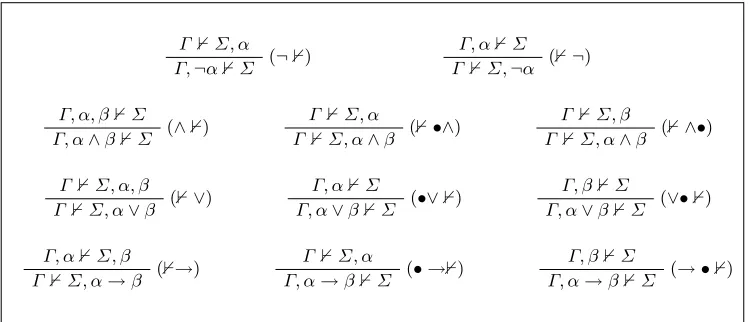
We start with the definition of Bonatti’s antisequent calculus AC from [3]. A related refutation calculus for first-order logic was previously developed by Tiomkin [23]. In AC we use antisequents Γ 0_{∆, where Γ, ∆ ⊆ L. Intuitively,}

Γ 0_{∆means that}W

∆does not follow fromV

Γ. Axioms ofAC are all sequents

Γ 0_{∆, whereΓ and∆are disjoint sets of propositional variables. The inference} rules ofAC are shown in Fig. 1. For this calculus, Bonatti [3] shows:

Γ 0_{Σ, α} (¬0)

Γ,¬α0_Σ

Γ, α0_Σ (0_¬)

Γ 0_Σ,¬α

Γ, α, β0Σ

(∧0)

Γ, α∧β0_Σ

Γ 0Σ, α

(0_•∧)

Γ 0_{Σ, α∧β}

Γ 0Σ, β

(0_∧•)

Γ 0_{Σ, α∧β}

Γ 0_{Σ, α, β} (0_∨)

Γ 0_{Σ, α∨β}

Γ, α0_Σ

(•∨0)

Γ, α∨β0_Σ

Γ, β0_Σ

(∨•0)

Γ, α∨β0_Σ

Γ, α0_{Σ, β}

(0_→)

Γ 0_{Σ, α→β}

Γ 0_{Σ, α}

(• →0)

Γ, α→β0_Σ

Γ, β0_Σ

(→ •0)

Γ, α→β0_Σ

Fig. 1.Inference rules of the antisequent calculusAC.

Theorem 4 (Bonatti [3]). The antisequent calculus AC is sound and com-plete.

Concerning the size of proofs in the antisequent calculus we observe: Proposition 5. The antisequent calculus AC is polynomially bounded.

Proof. Observe that the calculus contains only unary inference rules, each of which reduces the logical complexity of one of the contained formulae (if per-ceived bottom-up). Thus each use of an inference rule decrements the size of the formulae by at least one. After a linear number of steps we end up with only propositional variables which we cannot reduce any further. Each antisequent is of linear size, hence the complete derivation has quadratic size. ⊓⊔

The above observation is not very astounding, since, to verify Γ 0 _{∆ we} could alternatively guess assignments to the propositional variables inΓ and ∆

and thereby verify antisequents inNP_.

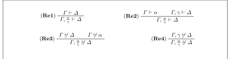
We now turn to the residual calculus RC of Bonatti and Olivetti [4]. Its objects areresidual sequents hW, Ri ⊢∆and residual antisequents hW, Ri0_∆ whereW, ∆⊆ L and R⊆ Lres_{. The intuitive meaning is that ∆ does}

(respec-tively does not) follow fromW using the residuesR. The rules ofRC comprise of the inference rules from Fig. 2 together with the rules ofLK andAC. How-ever, the use of rules from LK and AC is restricted to purely propositional (anti)sequents. For this calculus, Bonatti and Olivetti [4] showed:

Γ ⊢∆

(Re1)

Γ,α γ ⊢∆

Γ ⊢α Γ, γ⊢∆

(Re2)

Γ,α γ ⊢∆

Γ 6⊢∆ Γ 6⊢α

(Re3)

Γ,α γ 6⊢∆

Γ, γ6⊢∆

(Re4)

Γ,α γ 6⊢∆

Fig. 2.Inference rules of the residual calculusRC.

1. hW, Ri ⊢∆ is derivable in RC if and only if W

∆∈Cl(W, R); 2. hW, Ri0_{∆ is derivable in RC if and only if} W

∆ /∈Cl(W, R).

To bound the lengths of proofs in this calculus we exploit the property that residues only have to be used at a certain level and are not used to deduce any formulae afterwards (cf. Lemma 3). Using this we prove that the complexity of

RC is tightly linked to that of LK.

Lemma 7. There exist a polynomial p and a constant c such that sRC(n) ≤

p(n)·sLK(cn) and tRC(n)≤p(n)·tLK(cn).

Proof. The proof consists of two parts. First we will show the bounds stated above for sequents. In the second part we will then show that antisequents even admit polynomial-size proofs inRC.

Assume first that we want to derive the sequenthW, Ri ⊢∆, whereW, ∆⊆ L

and R ={r1, . . . , rk} is a set of residues withri = αi_γi. Let R′ ⊆R be minimal

with respect to the size |R′| such that hW, R′i ⊢ ∆. We may w.l.o.g. assume that R′ ={r1, . . . , rk′} and k′ ≤k. Furthermore, by Lemma 3, we may assume

that the rules ri are ordered in the way they are applied when computing the

setsCi. In particular, this means that for each i= 1, . . . , k′,

W ∪ {γ1, . . . , γi−1} ⊢αi

is a true propositional sequent for which we fix an LK-proof Πi. We augment

Πi by k′−iapplications of rule (Re1) to obtain

hW ∪ {γ1, . . . , γi−1},{ri+1, . . . , rk′}i ⊢α_i .

Let us call the proof of this sequentΠ_i′.

The proof tree depicted in Fig. 3 for derivinghW, Ri ⊢∆unfurls as follows. We start with an LK-proof for the sequent W ∪ {γ1, . . . , γk′} ⊢ ∆ and then

applyk′-times the rule (Re2) in the step

hW∪ {γ1, . . . , γi−1},{ri+1, . . . , rk′}i ⊢αi hW∪ {γ1, . . . , γi},{ri+1, . . . , rk′}i ⊢∆ hW∪ {γ1, . . . , γi−1},{ri, . . . , rk′}i ⊢∆

to reachhW, R′i ⊢∆. To derive the left prerequisite we use the proofΠ_i′. Finally we use k−k′ _{applications of the rule (Re1) to gethW, Ri ⊢∆.}

Our proof for hW, Ri ⊢ ∆ uses at most (k′ _{+ 1)·t}

LK(n) + k

′_(k′₊₁₎

2 +k

steps, i.e.,tRC(n)≤ O(n·tLK(n) +n2). Each sequent is of linear size. Hence,

Π′

1

Π′

2

Πk′′ hW∪ {γ1, . . . , γk′},∅i ⊢∆ (Re2) ..

.

hW∪ {γ1, γ2},{r3, . . . , rk′}i ⊢∆ (Re2) hW∪ {γ1},{r2, . . . , rk′}i ⊢∆

(Re2) hW, R′i ⊢∆

(Re1) ..

. hW, Ri ⊢∆

Fig. 3.Proof tree for the sequenthW, Ri ⊢∆in the residual calculus.

In the second part of the proof we will now show that any true antisequent has anRC-proof of polynomial size, thus concluding the proof. LethW, Ri0_∆ be the antisequent we wish to prove. Again, letR={r1, . . . , rk} withri = αi_γi,

and let {i1, . . . , iℓ}=I ⊆ {1, . . . , k} be a set of maximal cardinality such that

W ∪S

i∈I{γi}

0_{∆and letI}′_{={iℓ+1, . . . , ik}={1, . . . , k} \I.}

Because of hW, Ri 0 _{∆, the set I contains all indices i with αi ∈ Cl(W).} Therefore, for each j ∈ I′ we have W ∪S

i∈I{γi} 0 αj. We fix a

polynomial-size AC-proof Πj of this antisequent. Augmenting these proofs with ℓ

appli-cations of (Re4) we obtain a proof Π_j′ of

W,S

i∈I{ri}

0 _{αj. Similarly, as}

W ∪S

i∈I{γi}

0_{∆we get a polynomial-size proofΠ}′

k+1of

W,S

i∈I{ri}

0_∆. Now, the proof forhW, Ri0_{∆ends with the following application of (Re3)}

W,{ri1, . . . , rik−1}

0_∆

W,{ri1, . . . , rik−1}

0_αi

k hW,{ri1, . . . , rik}i0∆

More generally, for all choices ofs, twithℓ < s < t≤k+ 1 we use the (Re3)-step

W,{ri1, . . . , ris−1}

0_{αit W,{ri}

1, . . . , ris−1}

0_αis hW,{ri1, . . . , ris}i0αit

where we set αk+1 = W∆. After all these steps, it remains to derive the

an-tisequents hW,{ri1, . . . , riℓ}i 0 αit for ℓ < t ≤ k+ 1. But for these we have

already built the proofs Πt′. Therefore, we have constructed an RC-proof of hW, Ri0_{∆which apart from the AC-proofsΠt}′ _{uses onlyO(k}2_{) applications of} (Re3) and (Re4). As each antisequent in the proof is of linear size, we obtain a polynomial-sizeRC-proof of hW, Ri0_{∆. ⊓⊔} Let us remark that while theRC-proof of hW, Ri ⊢∆ in Fig. 3 is tree-like, this is not true for our dag-like RC-proof of hW, Ri 0 _{∆ constructed in the} second part of the proof of Lemma 7.

4 Proof Complexity of Credulous Default Reasoning

formLαor¬Lαwithα∈ L. A setE ⊆ Lsatisfies a constraintLαifα∈T h(E). Similarly, E satisfies ¬Lα ifα6∈T h(E).

We can now describe the calculus BOcred of Bonatti and Olivetti [4] for

credulous default reasoning. A credulous default sequent is a 3-tuplehΣ, Γ, ∆i, denoted by Σ;Γ|∼∆, where Γ = hW, Di is a default theory, Σ is a set of provability constraints and ∆is a set of propositional sentences. Semantically, the sequent Σ;Γ|∼∆ is true, if there exists a stable extension E of Γ which satisfies all of the constraints inΣandW

∆∈E. The calculusBOcred uses such

sequents and extendsLK,AC, and RC by the inference rules in Fig. 4.

Γ ⊢∆

(cD1) (Γ ⊆ Lres₎

; Γ|∼∆

Γ ⊢α Σ; Γ|_∼∆

(cD2) (Γ ⊆ Lres₎ Lα, Σ; Γ|∼∆

Γ 6⊢α Σ; Γ|_∼∆

(cD3) (Γ ⊆ Lres₎

¬Lα, Σ; Γ|∼∆

L¬βi, Σ; Γ|∼∆ (cD4)

Σ; Γ,α:β1...βn

γ |∼∆

¬L¬β1. . .¬L¬βn, Σ; Γ,α_γ|∼∆ (cD5)

Σ; Γ,α:β₁...βn

γ |∼∆

Fig. 4.Inference rules for the credulous default calculusBOcred.

For this calculus Bonatti and Olivetti [4] show the following:

Theorem 8 (Bonatti, Olivetti [4]). BOcred is sound and complete, i.e., a

credulous default sequent is true if and only if it is derivable in BOcred.

We now investigate lengths of proofs inBOcred. Our next lemma shows that

upper bounds on the proof size ofRC can be transferred to BOcred.

Lemma 9. For any functiont(n), if RC ist(n)-bounded, then BOcred isp(n)·

t(n)-bounded for some polynomialp. The same relation holds for the number of steps in RC and BOcred.

Proof. Let Σ;Γ|∼∆ be a true credulous default sequent. We will construct a

BOcred-derivation ofΣ;Γ|∼∆starting from the bottom with the given sequent.

Observe that we cannot use any of the rules (cD1) through (cD3) as long as Γ contains proper defaults with nonempty justification. Thus we first have to reduce all defaults to residues plus some set of constraints using (cD4) or (cD5). As one of these rules has to be applied exactly once for each appearance of some default in Γ we end up with Σ′;Γ′|∼∆, where |Σ′| is polynomial in

|Γ ∪Σ|andΓ′ is equal to Γ on its propositional part and contains some of the corresponding residues instead of the defaults from Γ. From this point on we can only use rules (cD2) and (cD3) until we have eliminated all constraints and then finally apply rule (cD1) once. Thus, BOcred-proofs look as shown in

RC

RC

RC _(cD1)

Γ′|_∼∆

(cD2) or (cD3)

σ;Γ′|∼∆

(cD2) or (cD3)

.. .

Σ′′;Γ′|∼∆

(cD2_{) or (}cD3₎

Σ′;Γ′|∼∆

(cD4_{) or (}cD5₎ ..

.

Σ;Γ|∼∆

Fig. 5.The structure of theBOcred-proof in Lemma 9

Combining Lemmas 7 and 9 we obtain our main result in this section stating a tight connection between the proof complexity ofLK and BOcred.

Theorem 10. There exist a polynomialpand a constantcsuch thatsLK(n)≤

sBOcred(n)≤p(n)·sLK(cn) andtLK(n)≤tBOcred(n)≤p(n)·tLK(cn).

In the light of this result, proving either non-trivial lower or upper bounds to the proof size of BOcred seems very difficult—as such a result would mean a

major breakthrough in propositional proof complexity (cf. [3, 17]).

4.1 On the Automatizability of BO_cred

Practitioners are not only interested in the size of a proof, but face the more complicated problem to actually construct a proof for a given instance. Of course, in the presence of super-polynomial lower bounds to the proof size this cannot be done in polynomial time. Thus, in proof search the best one can hope for is the following notion of automatizability:

Definition 11 (Bonet, Pitassi, Raz [6]). A proof system P for a language

L isautomatizable if there exists a deterministic procedure that takes as input a string x and outputs a P-proof of x in time polynomial in the size of the shortest P-proof ofx if x∈L. If x 6∈L, then the behaviour of the algorithm is unspecified.

For practical purposes automatizable systems would be very desirable. Search-ing for a proof we may not find the shortest one, but we are guaranteed to find one that is only polynomially longer. Unfortunately, forBOcred there are strong

limitations towards this goal as our next result shows:

Theorem 12. BOcred is not automatizable unless factoring integers is possible

in polynomial time.

Proof. First we observe that automatizability ofBOcred implies

automatizabil-ity of Frege systems. For this let ϕ be a propositional tautology. By assump-tion, we can construct a BOcred-proof of ∅|∼ϕ. This BOcred-proof contains an

automatizable unless Blum integers can be factored in polynomial time (a Blum integer is the product of two primes which are both congruent 3 modulo 4). ⊓⊔

4.2 A General Construction of Proof Systems for Credulous Default Reasoning

In this section we will explain a general method how to construct proof systems for credulous default reasoning. These proof systems arise from the canonical

Σp

2 algorithm for credulous default reasoning (Algorithm 1). Algorithm 1 first

guesses a generating setGextfor a potential stable extension and then verifies by

the stage construction from Theorem 1 that Gext indeed generates a stable

ex-tension which moreover contains the formulaϕ. Algorithm 1 is a Σp

2 procedure, i.e., it can be executed by a nondeterministic polynomial-time Turing machine

M with access to a coNP_{-oracle. The nondeterminism solely lies in line 1 and}

the oracle queries are made in lines 6 and 11 to the coNP_{-complete problem of}

propositional implication IMP ={hΨ, ϕi |Ψ ⊆ L, ϕ∈ L, and Ψ |=ϕ}.

Algorithm 1 A Σp

2 procedure for credulous default reasoning

Require: hW, Di,ϕ

1: guessD0⊆Dand letGext←W∪

n

γ|α:β γ ∈D0

o

2: Gnew←W

3: repeat

4: Gold←Gnew

5: for all α:β

γ ∈Ddo

6: if Gold|=αandGext6|=¬βthen

7: Gnew←Gnew∪ {γ}

8: end if

9: end for

10: untilGnew=Gold

11: if Gnew=GextandGext|=ϕthen

12: return true

13: else

14: return false

15: end if

Algorithm 1 can be converted into a proof system for credulous default reasoning as follows. We fix a propositional proof system P and define a proof systemCred(P) for credulous default reasoning where proofs are of the form

hW, D, ϕ,comp, q1, . . . , qk, a1, . . . , aki .

Here comp is a computation of M on input hW, D, ϕi and q1, . . . , qk are the

queries to IMP during this computation. If the IMP-query qi = hΨi, ϕii is

answered positively, thenai is aP-proof of

V

ψ∈Ψiψ

→ϕi, otherwiseai is an

assignment falsifying this formula. For this proof system we obtain the following bounds:

Proof. The first inequality holds because we can useCred(P) to prove propo-sitional tautologiesϕby choosingW =D=∅.

For the second inequality, we observe that Algorithm 1 has quadratic run-ning time. In particular, a computation of Algorithm 1 contains at most a quadratic number of queries to IMP. Each of these queries is of linear size because it only consists of formulae from the input. If the query is answered positively, then we have to supply a P-proof and there exists such a P-proof of size ≤sP(n). For a negative answer we just include an assignment of linear

size. This yields sCred(P)(n)≤ O(n2sP(n)). ⊓⊔

Theorem 13 tells us that proving lower bounds for proof systems for cred-ulous default reasoning is more or less the same as proving lower bounds to propositional proof systems. In particular, we get:

Corollary 14. There exists a polynomially bounded proof system for credulous default reasoning if and only if there exists a polynomially bounded propositional proof system.

5 Lower Bounds for Skeptical Default Reasoning

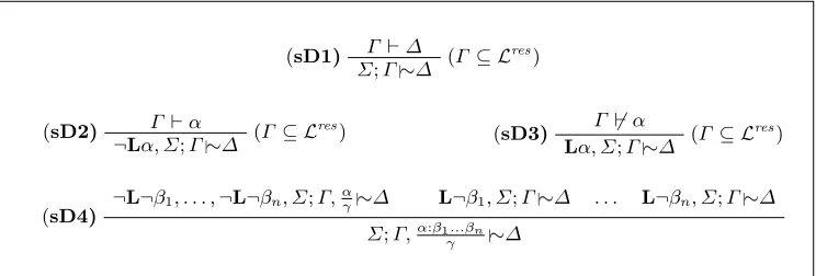
Bonatti and Olivetti [4] introduce two calculi for skeptical default reasoning. As before, objects are sequents of the formΣ;Γ|_∼∆, whereΣis a set of constraints,

Γ is a propositional default theory, and∆is a set of propositional formulae. But now, the sequentΣ;Γ|∼∆is true, ifW

∆holds in allextensions ofΓ satisfying the constraints inΣ.

The first calculus BOskep consists of the defining axioms of LK and AC,

the inference rules of LK, AC, RC, and the rules from Fig. 6. Bonatti and

Γ ⊢∆

(sD1) (Γ ⊆ Lres₎

Σ;Γ|_∼∆

Γ ⊢α

(sD2) (Γ ⊆ Lres₎

¬Lα, Σ;Γ|∼∆

Γ 6⊢α

(sD3) (Γ ⊆ Lres₎ Lα, Σ;Γ|∼∆

¬L¬β1, . . . ,¬L¬βn, Σ;Γ,α_γ|∼∆ L¬β1, Σ;Γ|∼∆ . . . L¬βn, Σ;Γ|∼∆

(sD4)

Σ;Γ,α:β1...βn

γ |∼∆

Fig. 6.Inference rules for the skeptical default calculusBOskep.

Olivetti show that each true sequent is derivable inBOskep,i.e., the calculus is

sound and complete. However, they already remark that proofs in BOskep are

of exponential size in the number of default rules in the sequent. This is due to the residual rules for they cannot be applied unless all defaults with nonempty justifications have been eliminated using rule (sD4).

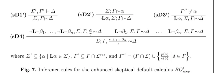
(sD3′) and rule (sD4) is kept (see Fig. 7). Bonatti and Olivetti prove sound-ness and completesound-ness forBO′

skep. Moreover, they show thatBOskep′ is

exponen-tially separated from BOskep, i.e., there exist sequents (Sn)n≥1 which require

exponential-size proofs in BOskep but have linear-size derivations inBOskep′ . In

Σ′, Γ′⊢∆

(sD1’)

Σ;Γ|∼∆

Σ;Γ|∼α (sD2’)

¬Lα, Σ;Γ|∼∆

Γ′′6⊢α

(sD3’)

Lα, Σ;Γ|∼∆

¬L¬β1, . . . ,¬L¬βn, Σ;Γ,α_γ|∼∆ L¬β1, Σ;Γ|∼∆ . . . L¬βn, Σ;Γ|∼∆ (sD4)

Σ;Γ,α:β₁...βn

γ |∼∆

whereΣ′⊆ {α|Lα∈Σ},Γ′⊆Γ ∩ Lres_{, andΓ}′′_{= (Γ ∩ L)∪}np(δ)

c(δ)

˛ ˛ ˛δ∈Γ

o .

Fig. 7.Inference rules for the enhanced skeptical default calculusBOskep′ .

our next result we will show an exponential lower bound to the proof length (and therefore also to the proof size) in the enhanced skeptical calculusBO_skep′ . Theorem 15. The calculus BO′

skep has exponential lower bounds to the lengths

of proofs. More precisely, there exist sequents Sn of size O(n) such that every BO_skep′ -proof of Sn uses 2Ω(n) steps. Therefore, sBO′

skep(n), tBOskep′ (n)∈2

Ω(n)_.

Proof. (Sketch)We construct a sequence (Sn)n≥1 = (Σn;Γn|∼ψn)n≥1 such that

for some constant c, every BO′

skep-proof of Sn has length at least 2Ω(n). We

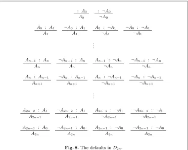
chooseΣn=∅,ψn=A2n, andΓn=h∅, D2ni, whereD2nconsists of the defaults

listed in Fig. 8. The default theoryΓnpossesses 2n+1stable extensions. Observe

that each of these contains A2n, but that each pair of stable extensions differs

in truth assigned to the propositional variablesA0, . . . , An. We claim that every

proof of Snhas exponential length inn. More precisely, we will show that rule

(sD4) has to be applied an exponential number of times.

We point out that our argument does not only work against tree-like proofs, but also rules out the possibility of sub-exponential dag-like derivations for

D2n|∼A2n. The lower bound is obtained from the fact that to deriveA2n, we have

to derive Ai and ¬Ai for eachn < i <2n, each of which can only be achieved

from ancestors with mutually different proof constraints. This, by definition of

BOskep, leads to mutually disjoint sets of ancestor sequents.

The complete proof of the theorem is contained in the appendix. ⊓⊔

6 Conclusion

In this paper we have shown that with respect to lengths of proofs, proof systems for credulous default reasoning and for propositional logic are very close to each other. Although deciding credulous default sequents is presumably harder than deciding tautologies (the former is Σp

2-complete [13], while the latter is

complete for coNP_{), the difference disappears when we want to prove these}

: A0

A0

: ¬A0

¬A0

A0 : A1

A1

¬A0 : A1

A1

A0 : ¬A1

¬A1

¬A0 : ¬A1

¬A1

.. .

An−1 : An

An

¬An−1 : An

An

An−1 : ¬An ¬An

¬An−1 : ¬An ¬An

An : An−1

An+1

¬An : An−1

An+1

An : ¬An−1

¬An+1

¬An : ¬An−1

¬An+1

.. .

A2n−2 : A1

A2n−1

¬A2n−2 : A1

A2n−1

A2n−2 : ¬A1

¬A2n−1

¬A2n−2 : ¬A1

¬A2n−1

A2n−1 : A0

A2n

¬A2n−1 : A0

A2n

A2n−1 : ¬A0

A2n

¬A2n−1 : ¬A0

A2n

Fig. 8.The defaults inD2nin the proof of Theorem 15.

For skeptical reasoning this is less clear. While skeptical default reasoning has polynomially bounded proof systems if and only if this holds for TAUT, we leave open whether this equivalence extends to other bounds. However, in the light of our exponential lower bound for BO′

skep (Theorem 15), searching for

natural proof systems for skeptical default reasoning with more concise proofs will be a rewarding task for future research.

In this direction Bonatti and Olivetti [4] themselves introduced two rules to supplement their enhanced calculus. These are the cut rule

Σ;Γ|∼α Σ;Γ, α|∼∆

(Cut)

Σ;Γ|∼∆

and the following version of the rule (sD4)

Σ0, Σ;Γ,α_γ|∼∆ Σ1, Σ;Γ|∼∆ . . . Σn, Σ;Γ|∼∆

(sD4′₎

Σ;Γ,α:β1...βn

γ |∼∆

whereΣi=L¬βπ(i),¬L¬βπ(i+1), . . . ,¬L¬βπ(n) for an arbitrary permutationπ

of {1, . . . , n}. While it is not hard to see that our lower bound in Theorem 15 still remains true if we add (sD4′) to BO_skep′ , we leave open the problem to show super-polynomial lower bounds in the presence of the cut rule.

Acknowledgement

References

1. G. Amati, L. C. Aiello, D. M. Gabbay, and F. Pirri. A proof theoretical approach to default reasoning I: Tableaux for default logic. Journal of Logic and Computation, 6(2):205–231, 1996.

2. G. Antoniou. A tutorial on default logics. ACM Comput. Surv., 31(4):337–359, 1999. 3. P. A. Bonatti. A Gentzen system for non-theorems. Technical Report CD/TR 93/52,

Christian Doppler Labor f¨ur Expertensysteme, 1993.

4. P. A. Bonatti and N. Olivetti. Sequent calculi for propositional nonmonotonic logics. ACM Transactions on Computational Logic, 3(2):226–278, 2002.

5. M. L. Bonet, S. R. Buss, and T. Pitassi. Are there hard examples for Frege systems? In P. Clote and J. Remmel, editors,Feasible Mathematics II, pages 30–56. Birkh¨auser, 1995. 6. M. L. Bonet, T. Pitassi, and R. Raz. On interpolation and automatization for Frege

systems. SIAM Journal on Computing, 29(6):1939–1967, 2000.

7. M. Cadoli and M. Schaerf. A survey of complexity results for nonmonotonic logics.Journal of Logic Programming, 17(2/3&4):127–160, 1993.

8. S. A. Cook and R. A. Reckhow. The relative efficiency of propositional proof systems. The Journal of Symbolic Logic, 44(1):36–50, 1979.

9. J. Dix, U. Furbach, and I. Niemel¨a. Nonmonotonic reasoning: Towards efficient calculi and implementations. In Handbook of Automated Reasoning, pages 1241–1354. Elsevier and MIT Press, 2001.

10. U. Egly and H. Tompits. Proof-complexity results for nonmonotonic reasoning. ACM Transactions on Computational Logic, 2(3):340–387, 2001.

11. D. Gabbay. Theoretical foundations of non-monotonic reasoning in expert systems. In Logics and Models of Concurrent Systems, pages 439–457. Springer-Verlag, Berlin Heidel-berg, 1985.

12. G. Gentzen. Untersuchungen ¨uber das logische Schließen. Mathematische Zeitschrift, 39:68–131, 1935.

13. G. Gottlob. Complexity results for nonmonotonic logics. Journal of Logic and Computa-tion, 2(3):397–425, 1992.

14. P. Hrubeˇs. On lengths of proofs in non-classical logics. Annals of Pure and Applied Logic, 157(2–3):194–205, 2009.

15. E. Jeˇr´abek. Frege systems for extensible modal logics.Annals of Pure and Applied Logic, 142:366–379, 2006.

16. E. Jeˇr´abek. Substitution Frege and extended Frege proof systems in non-classical logics. Annals of Pure and Applied Logic, 159(1–2):1–48, 2009.

17. J. Kraj´ıˇcek.Bounded Arithmetic, Propositional Logic, and Complexity Theory, volume 60 ofEncyclopedia of Mathematics and Its Applications. Cambridge University Press, Cam-bridge, 1995.

18. S. Kraus, D. J. Lehmann, and M. Magidor. Nonmonotonic reasoning, preferential models and cumulative logics. Artificial Intelligence, 44(1–2):167–207, 1990.

19. D. Makinson. General theory of cumulative inference. InProc. 2nd International Work-shop on Non-Monotonic Reasoning, pages 1–18. Springer-Verlag, Berlin Heidelberg, 1989. 20. V. W. Marek and M. Truszczy´nski.Nonmonotonic Logics—Context-Dependent Reasoning.

Springer-Verlag, Berlin Heidelberg, 1993.

21. R. Reiter. A logic for default reasoning. Artificial Intelligence, 13:81–132, 1980.

22. V. Risch and C. Schwind. Tableaux-based characterization and theorem proving for default logic. Journal of Automated Reasoning, 13(2):223–242, 1994.

Technical Appendix

The appendix contains the full proof of Theorem 15 which was only briefly sketched in the main part of the paper.

Theorem 15. The calculus BO′

skep has exponential lower bounds to the lengths

of proofs. More precisely, there exist sequents Sn of size O(n) such that every BO′

skep-proof of Sn uses 2Ω(n) steps. Therefore,sBO′

skep(n), tBOskep′ (n)∈2

Ω(n)_.

Proof. We construct a sequence (Sn)n≥1 = (Σn;Γn|∼ψn)n≥1 such that for some

constantc, everyBO_skep′ -proof ofSnhas length at least 2Ω(n). We choose Σn= ∅, ψn = A2n, and Γn = h∅, D2ni, where D2n consists of the defaults listed in

Fig. 8. The default theory Γn possesses 2n+1 stable extensions. Observe that

each of these contains A2n, but that each pair of stable extensions differs in

truth assigned to the propositional variablesA0, . . . , An. We claim that every

: A0

A0

: ¬A0

¬A0

A0 : A1

A1

¬A0 : A1

A1

A0 : ¬A1

¬A1

¬A0 : ¬A1

¬A1

.. .

An−1 : An

An

¬An−1 : An

An

An−1 : ¬An ¬An

¬An−1 : ¬An ¬An

An : An−1

An+1

¬An : An−1

An+1

An : ¬An−1

¬An+1

¬An : ¬An−1

¬An+1

.. .

A2n−2 : A1

A2n−1

¬A2n−2 : A1

A2n−1

A2n−2 : ¬A1

¬A2n−1

¬A2n−2 : ¬A1

¬A2n−1

A2n−1 : A0

A2n

¬A2n−1 : A0

A2n

A2n−1 : ¬A0

A2n

¬A2n−1 : ¬A0

A2n

Fig. 8.The defaults inD2n.

proof ofSn has exponential length inn. More precisely, we will show that rule

(sD4) has to be applied an exponential number of times.

To this end, letΠ be aBO_skep′ -proof ofD2n|∼A2n. We show that Π has to

contain an application of (sD4) to a default rule deriving Ai or ¬Ai for any

sequent

Σ;D, R|∼A2n (1)

such that Σ is consistent and D2n can be partitioned into three sets I1,I2,I3

1. ¬L¬j(δ)∈Σ and p_c((_δδ)₎ ∈R ifδ∈I1,

2. L¬j(δ)∈Σ ifδ ∈I2,

3. δ∈D ifδ∈I3, and

4. {Ai,¬Ai} ∩ {c(δ)|δ∈I1}=∅for somen < i≤2n

To prove this claim, let Σ;D, R|∼A_2n be a sequent as stated above and

n < i ≤ 2n be such that {Ai,¬Ai} ∩ {c(δ) | δ ∈ I1} = ∅. Suppose that Π

does not contain any application of (sD4) to default rules deriving Ai or¬Ai.

Consequently, Σ;D, R|∼A_2n is derived by an application of (sD1’), (sD2’), (sD3’) or (sD4) to a default rule not derivingAi or¬Ai. We distinguish among

these possibilities.

(sD1’) SupposeΣ;D, R|∼A2nwere derived by an application of (sD2’), thenΠ

had to contain the the sequent Σ′, R⊢ A2n, where Σ ⊆ {A2n−k,¬A2n−k |

n ≤ k ≤ 2n}. By the fourth condition, {Ai,¬Ai} ∩ {c(δ) | δ ∈ I1} = ∅.

Hence,Rcannot contain any of the residual rules αi−1

αi withαj ∈ {Aj,¬Aj}.

Consequently,Σ′;R|_∼A2n cannot be closed.

(sD2’) IfΣ;D, R|∼A_2nwere derived by an application of (sD2’), thenΠhad to contain the antecedentΣ′, D, R|∼¬α2n−k, where α2n−k ∈ {A2n−k,¬A2n−k}

withn ≤k ≤2n and Σ′ := Σ\ {¬L¬α2n−k}. However, Σ′;D, R|∼¬α2n−k

could in turn only be closed by using either of the default rules A2n−k−1 : ˜α2n−k _,

˜

α2n−k

¬A2n−k−1 : ˜α2n−k _, ˜

α2n−k

where ˜α2n−k ≡ ¬α2n−k: no other rules derives ¬A2n−k. Say that Π

con-tains an application of the first rule. By consistency of Σ, A2n−k−1: ˜α2n−k ˜

α2n−k

has to be contained in D. Suppose w.l.o.g. that Π contains this applica-tion in the previous step of Π. Then we obtain as the right ancestor se-quent Σ′;L¬α˜2n−k;D′, R|∼α˜2n−k, where D′ := D\

n_A

2n−k−1: ˜α2n−k ˜

α2n−k

o

. But

Σ′,L¬α˜2n−k;D′, R|∼α˜2n−k cannot be closed: The only default rule being

able to derive ˜α2n−k remaining inD′ has a premise that is contradictory to

the premise ofA2n−k−1: ˜α2n−k ˜

α2n−k . By soundness ofBO

′

skep, the ability to close this

sequent would therefore contradict the consistency of D2n. The case that

Π contains an application of the second rule, ¬A2n−k−1: ˜α2n−k ˜

α2n−k , is completely

analogous.

(sD3’) Similarly, if the sequent Σ;D, R|∼A₂n were derived by an application

of the rule (sD3’), thenΠ contained the sequent D′, R0_{¬αl for some αl} such that L¬αl ∈ Σ, where D′ =

n

p(δ) c(δ)

δ∈D

o

. But if D′, R 0 _{¬αl were} true, then there had to exist an 0 ≤ j ≤ l such that neither of the rules

Aj−1:αj

αj ,

¬Aj−1:αj

αj , where αj ∈ {Aj,¬Aj} forj < l, nor one of their residues

could be contained inD∪R. Consequently,Π would again have to contain the proof constraints L¬αj,L¬¬αj ∈ Σ, contradictory to the consistency

ofΣ.

(sD4’) Suppose that Σ;D, R|_∼A2n is derived by an application of (sD4) to

the default rule αk−1:α2n−k

αk ∈ Dwith αj ∈ {Aj,¬Aj} and n < k6=i. Then

Π contains the two ancestor sequents Σ,¬L¬α2n−k;D, R,α_αk−1

k |∼A2n and

Σ,L¬α2n−k;D, R|∼A2n. But asΣ,¬L¬α2n−k;D, R,αk_α−1

contain any residual rule deriving Ai or ¬Ai, the same arguments as for

Σ;D, R|∼A_2n apply.

Concluding, the containment ofΣ;D, R|∼A2nin Π enforces an application

of (sD4) to a default rule with conclusion Ai or¬Ai. This yields the ancestor

sequentsΣ,¬L¬α2n−i;D, R,αi_αi−1|∼A2nand Σ,L¬α2n−i;D, R|∼A2n. The latter

of these still satisfies the requirements of (1). Thus, by the same arguments as above, Π has to contain an application of (sD4) to a default rule α′i−1:α′2n−i

α′

i ,

whereα′_i ≡ ¬αiandα2′n−i ≡ ¬α2n−i. Each of these applications yields a sequent

satisfying (1) unless for these {Ai,¬Ai} ∩ {c(δ) | δ ∈ I1} 6= ∅ holds for all

n < i≤2n; however, with mutually different proof constraints.

Summing up, to prove D2n|∼A2n,Π has to contain 22n−i+1 applications of

(sD4) to default rules with conclusionAi or¬Ai. Therefore, every proof of Sn

has length at least 2Ω(n)_{. ⊓⊔}

We point out that the above argument does not only work against tree-like proofs, but also rules out the possibility of sub-exponential dag-like derivations forD2n|∼A2n. The lower bound is obtained from the fact that to deriveA2n, we

have to derive residual rules concludingAi and ¬Ai for each n < i≤2n, each