Visualization of parameter space for image analysis

This is a repository copy of

Visualization of parameter space for image analysis

.

White Rose Research Online URL for this paper:

http://eprints.whiterose.ac.uk/74328/

Article:

Pretorius, AJ, Bray, MA, Carpenter, AE et al. (1 more author) (2011) Visualization of

parameter space for image analysis. IEEE Transactions on Visualization and Computer

Graphics, 17 (12). 2402 - 2411 . ISSN 1077-2626

https://doi.org/10.1109/TVCG.2011.253

[email protected]

https://eprints.whiterose.ac.uk/

Reuse

Unless indicated otherwise, fulltext items are protected by copyright with all rights reserved. The copyright

exception in section 29 of the Copyright, Designs and Patents Act 1988 allows the making of a single copy

solely for the purpose of non-commercial research or private study within the limits of fair dealing. The

publisher or other rights-holder may allow further reproduction and re-use of this version - refer to the White

Rose Research Online record for this item. Where records identify the publisher as the copyright holder,

users can verify any specific terms of use on the publisher’s website.

Takedown

If you consider content in White Rose Research Online to be in breach of UK law, please notify us by

Visualization of Parameter Space for Image Analysis

A. Johannes Pretorius, Mark-Anthony P. Bray, Anne E. Carpenter, and Roy A. Ruddle

Abstract— Image analysis algorithms are often highly parameterized and much human input is needed to optimize parameter set-tings. This incurs a time cost of up to several days. We analyze and characterize the conventional parameter optimization process for image analysis and formulate user requirements. With this as input, we propose a change in paradigm by optimizing parameters based on parameter sampling and interactive visual exploration. To save time and reduce memory load, users are only involved in the first step - initialization of sampling - and the last step - visual analysis of output. This helps users to more thoroughly explore the parameter space and produce higher quality results. We describe a custom sampling plug-in we developed for CellProfiler - a popular biomedical image analysis framework. Our main focus is the development of an interactive visualization technique that enables users to analyze the relationships between sampled input parameters and corresponding output. We implemented this in a prototype called Paramorama. It provides users with a visual overview of parameters and their sampled values. User-defined areas of interest are presented in a structured way that includes image-based output and a novel layout algorithm. To find optimal parameter settings, users can tag high- and low-quality results to refine their search. We include two case studies to illustrate the utility of this approach.

Index Terms—Information visualization, visual analytics, parameter space, image analysis, sampling.

1 INTRODUCTION

There is a long tradition of visual analysis in the life sciences. For nearly four centuries scientists have peered down microscopes to do their work. During the past two decades biomedical researchers in-creasingly started scrutinizing digital images on computer monitors due to a shift toward virtual microscopy [6]. Today, high-throughput technologies and imaging techniques allow scientists to automate ex-periments and capture large result sets as digital images [27]. Automa-tion is essential to analyze the vast quantities of biomedical images that scientists generate. Such algorithms automatically identify objects -such as cell nuclei - and compute associated metrics - -such as the area occupied by each cell. In aggregate, metrics of a large collection of experiments can be used for rigorous statistical analysis.

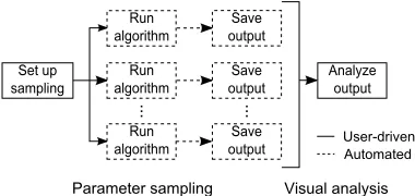
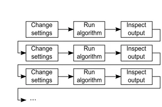
Image analysis algorithms are often highly parameterized and con-siderable human input is needed to optimize parameter settings. Fig-ure 1 illustrates the conventional approach of “parameter tweaking” by trial and error. Users start with a set of test images as input. They supply input parameter settings, initialize and wait for algorithms to execute, and inspect the output. Output is judged qualitatively, input settings are changed, and the process repeated until satisfactory results are achieved. At this point, users apply the algorithms and the settings arrived at to large collections of images that are similar to their test set. Parameter optimization presents a major usability challenge, which we attribute to:

• Time cost.Due to multiple input parameters, algorithm process-ing time, interruptions caused by waitprocess-ing for algorithms to exe-cute, and the number of iterations typically required, it can take days to identify appropriate settings.

• Memory load.The interruptions described above require users to rely on memory recall to compare current output with previous results. This is compounded for work spread over multiple days.

• A. Johannes Pretorius is with the School of Computing, University of Leeds, E-mail: [email protected].

• Mark-Anthony P. Bray is with the Broad Institute of MIT and Harvard, Email: [email protected].

• Anne E. Carpenter is with the Broad Institute of MIT and Harvard, Email: [email protected].

• Roy A. Ruddle is with the School of Computing, University of Leeds, E-mail: [email protected].

Manuscript received 31 March 2011; accepted 1 August 2011; posted online 23 October 2011; mailed on 14 October 2011.

For information on obtaining reprints of this article, please send email to: [email protected].

Run algorithm

Inspect output Change

settings

Run algorithm

Inspect output Change

settings

Run algorithm

Inspect output Change

settings

...

Fig. 1. The conventional approach for parameter optimization. Based on a qualitative assessment of current output, users iteratively change parameter settings and run algorithms to generate new output. This process is repeated until the output quality is satisfactory.

The above results in inadequate exploration of parameter space and the quality of results produced by image analysis algorithms suffers.

Machine-learning algorithms are one approach to potentially min-imize user overhead in achieving good object identification results. Users mark up regions of interest in several images, which the algo-rithms use to create complex classifiers that can recognize similar re-gions in other images. In the experience of domain experts, however, superior results can only be achieved using specific algorithms, when prior knowledge is available about the image, the objects, and their features (size and appearance). Also, machine learning approaches require a substantial amount of hand-labeling of images.

We present an alternative approach based on sampling and interac-tive visualization. In Section 2, we summarize related research before outlining CellProfiler - a popular image analysis framework - in Sec-tion 3. We discuss our work in SecSec-tion 4. This includes a requirements analysis (Section 4.1), a high-level strategy (Section 4.2), a custom plug-in for CellProfiler to sample parameter space (Section 4.3), and an interactive visualization technique for sampled parameter space and related output (Section 4.4). We validate our approach with two case studies in Section 5. We conclude and outline future work in Section 6.

2 RELATED WORK

The challenge of understanding the relationships between input pa-rameters and output underlies much of engineering design and applied science. Users are interested in exploring the mapping p1, ...,pn→

Linked charts. Tweedie et al were among the first to apply interac-tive visualization to parameter optimization [24]. Parameters and out-comes are represented asn+minteractive histograms. The domains of the parameters and outcomes are binned and a specific mapping is represented byn+mmarks, one on each histogram. When a mark is selected, it and all others associated with that mapping are high-lighted. Users can interactively specify a range for every parameter and outcome. This results in marks of mappings for which one or more dimensions fall outside this range being dimmed out.

In later work, Tweedie and Spence extended this approach to pro-section matrices [25]. These are linked 2D scatterplots, each with an associated third dimension on which users can specify an active range. Mappings for which one or more dimension fall outside these ranges are not shown on the scatterplots. Although more complex than his-tograms the underlying approach is identical: mappings are shown on multiple linked charts and are highlighted or dimmed out in real-time based on user interaction with the ranges of parameters and outcomes. Linked charts improve on conventional parameter optimization by showing an entire collection of results at one time. The dynamic querying capabilities enable users to investigate different scenarios. Moreover, users can quickly specify requirements on outcomes to identify those mappings for which the requirements are satisfied. In this way both time cost and memory load are addressed. Unfor-tunately, when considered in the context of image analysis, linked charts have a major drawback. By design there is the assumption that outcomes are ordinal and that users’ analyses are based on quantitative judgments of ranges on the charts’ axes. This makes them unsuitable for considering image-based output where judgments are qualitative.

Exploration graphs.Instead of focusing on the mapping between pa-rameters and outcomes, the changes in parameter values and their influence on outcomes can be emphasized. Ma took this approach by visualizing the parameter search process as a directed graph [15]. The aim is to assist users in finding rendering parameter settings for computer graphics scenes. Users start with the rendering that results from the default parameter settings shown as a thumbnail. When they change a parameter’s value, a new scene is rendered and displayed as another thumbnail. The change in a parameter’s value is represented by a directed edge connecting the initial scene to the new one.

The VisTrails visualization management system uses exploration graphs for history management [2, 4]. As different visualizations of a scientific data set are generated a history tree is maintained and shown to users. Users can select any node in the tree to view the correspond-ing visualization and proceed to change its parameter values. Like Ma’s work, such a change is shown by a new edge that leads to a child node that represents the new visual outcome.

An exploration graph enhances the parameter optimization process by serving as an external memory aid, augmenting each iteration in Figure 1 with a node representing the outcome. All outcomes that users have considered, as well as the exploration paths that led them there, are available in visual form. Using the graph, users are able to refine promising outcomes by introducing further parameter changes. If headed down a dead end, they can revisit a previous result and try other parameter changes to explore more of the parameter space. However, exploration graphs depend on laborious user interaction to explore parameter space. The exploration process is still linear and time cost remains an issue. This can be addressed by enabling users to script iterations over parameter values as in VisTrails [4], but assumes users are competent to write programming code. Because exploration graphs are not structured based on parameter values, it is difficult for users to interpret the analysis outcomes in the context of the parameter space.

Structured galleries.A number of techniques have been developed to present image-based outcomes in a structured fashion. Jankun-Kelly and Ma developed a technique based on a spreadsheet metaphor [10], again to investigate the influence of rendering parameters on computer graphics scenes. Pairs of parameters define a two-dimensional table with their domains, respectively, defining the coordinates of the

x-and y-axes. Renderings that result from a specific pair of settings are shown at the intersection of these two coordinates. All other parame-ters are fixed to constants. When users want to consider an additional parameter they assign a fixed value to one of the currently active pa-rameters. Next, the visualization is rotated in 3D before snapping to a new system of 2D axes that includes the newly selected parameter.

Further examples of structured galleries can be found in the work of Marks et al [16]. Instead of structuring outcomes based on input pa-rameter values, they focus on perceptually recognizable differences of outcomes. Underlying visual representations is a complex mechanism that considers distance metrics of perceptual properties. Parameter settings are chosen so that outcomes are perceptually well-distributed. One representation Marks et al developed is based on a hierarchical partitioning of the graph where edge weights represent the perceptual distances between rendered scenes. Users interactively explore the hierarchy as follows. First, they are shown a row of thumbnails cor-responding to the highest level of the hierarchy; perceptually the most coarse division of results. When they select one of these thumbnails its children, which are more similar, are shown on a second row of the hierarchy. The same approach can be applied repeatedly to converge on a result that satisfies users. Marks et al also developed a second representation based on a low-dimensional projection of outcomes in 2D. By employing multidimensional scaling on the distance metrics between outcomes, scenes that are similar map to positions close to each other on a 2D projection.

The above approaches offer a step up from conventional parameter optimization by either structuring outcomes based on the input parameter space or on a notion of their perceptual similarities. Both approaches offload some of the users’ memory load. However, due to the high degree of interaction required to consider multiple parameters, Jankun-Kelly and Ma’s approach retains much of the search by trial and error associated with the process illustrated in Figure 1. In the case of Marks et al, perceptually similar outcomes are conveniently mapped close to each other, but the relationships with input parameter settings are not always clear. Because similarity metrics have to be devised for each instance of a design problem, Marks et al concede that using their approach for more general problems, or even a class of problems, is difficult.

Preset landscapes.Van Wijk and Van Overveld introduced an innova-tive approach for parameter space exploration based on presets [26]. A preset serves as a reference point in parameter space and is defined as a vector of sizenthat contains a value for eachpi. Presets are visually represented as landmarks on a 2D plane that represents the parame-ter space. An outcome is also represented by an icon on this plane. Like the preset landmarks this icon can be moved. To compute the outcome, a linear combination of the inverse distances from the preset landmarks to the outcome is calculated.

Unless multiple outcomes are shown on the plane, exploration by presets does not alter the linear nature of conventional parameter op-timization (see Figure 1). Also, memory load is not significantly re-duced because users cannot readily compare different outcomes. An-other fundamental limitation of preset landscapes is that they require meaningful presets to have been defined. This is a valid assumption in the case of audio mixing, as Van Wijk and Van Overveld show, where it is logical to consider different musical instruments as presets. For image analysis, however, finding suitable presets amounts to another parameter optimization problem.

3 CELLPROFILER

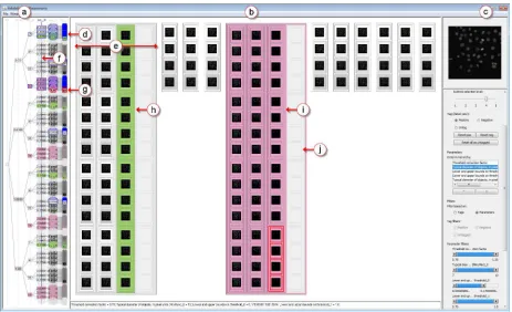
Fig. 2. (a) The CellProfiler user interface [5, 13]. A pipeline, with its constituent modules, is shown at the left of this interface. The input parameters of the selected module are shown at the right of the interface. (b) Parameter sampling in CellProfiler. A new plug-in automatically detects and lists all continuous parameters for a user-selected module. Users indicate which of these parameters to sample and for these they specify a range and the number of samples to compute. Next, the plug-in automatically performs sampling, computes all combinations of sampled values, executes the pipeline for each unique combination, and saves the outcome to disk.

Explorer [7] and ParaView [20]. A pipeline consists of a linear ar-rangement of processing modules. A module can accept input data - in the form of images or previously identified objects - from any module that precedes it. Moreover, a module performs a specific and well-defined operation on its data. A typical CellProfiler pipeline will contain modules for loading images, for correcting illumination, for identifying objects, and for computing measurements for these objects. As shown in Figure 2(a), a pipeline and its constituent modules are displayed at the left of the CellProfiler user interface. Users can add, remove, or rearrange modules. Users are required to provide settings for the input parameters of each module in a pipeline. When a module is selected, its parameters are shown at the right of the user interface where users specify parameter values. A typical pipeline consists of 10–20 modules, each with 5–20 parameters, yielding approximately 150–200 parameters in total. As we show in Section 4.1, a subset of these parameters receive the most attention.

4 APPROACH

To address the issues associated with parameter optimization raised in Section 1 (time cost and memory load, leading to inadequate explo-ration of parameter space and suboptimal quality), we analyzed the requirements of CellProfiler users. Based on this, we devised a high-level strategy that required work on two fronts. First, we developed a CellProfiler plug-in that samples the input parameter space and gener-ates corresponding output. Second, we developed a visualization tool to let users interactively explore the data generated by our sampler.

4.1 Analysis of user requirements

We interviewed experienced assay developers at the Broad Institute of MIT and Harvard. These experts regularly use CellProfiler and frequently assist and train less experienced users. We also observed novice users at a hands-on introductory workshop on CellProfiler.

Requirement 1.Complex biomedical research questions involving im-age analysis can usually be reduced to finding biological objects - such as cell nuclei - and to deriving simple statistics for these - such as the area occupied by each cell. To do so, users need support to effec-tively and efficiently identify a suitable set of parameter settings to get high-quality results from a representative test image. Once users have confidence in these settings, they will proceed to run a pipeline with these values to automatically analyze a large collection (hundreds to

millions) of similar images (high-throughput analysis). The results, when analyzed, allow them to answer their real research questions. Typically, this involves identifying cases where cells deviate from the norm in a particular way.

The above analysis enabled us to characterize the conventional ap-proach to parameter optimization shown in Figure 1. Our assay de-veloper collaborators immediately recognized the linear nature of the description and readily agreed that it was an accurate depiction of how users proceed to identify suitable parameter settings for CellProfiler. They confirmed that this approach presents a usability challenge (see Section 1) and explained that parameter optimization can typically re-quire anything from tens of minutes to two days’ work.

It is generally not possible to generate image analysis output in real-time. Algorithms are often complex and rarely have linear complexity. In practice, algorithms incur a delay of a few seconds, in the best case, to several hours, in the worst case. Image size also has an influence on the delay users can expect and as image resolution increases - for example, histology images can measure 80,000×100,000 pixels [23] - time delays will be part of image analysis for the foreseeable future. This presents two problems. First, while users wait for algorithms to execute, they are not adding value. Second, waiting for algorithms to finish interrupts their train of thought when optimizing parameters.

Our analysis of the parameter optimization process and the algorithms involved led us to formulate a first user requirement:

R1.Turn the linear and restricted process of parameter optimization into a more unconfined real-time analysis experience. Support users by separating the time-consuming image analysis processing - where their attention is not required - from the specification of input parameters and the inspection of output.

Requirement 2. We next turned our attention to the input parameters. Our analysis revealed three parameter classes:

• Aliases. Users are required to supply text labels for images or identified objects. Such aliases are used to refer to images or ob-jects to operate on in downstream modules. Aliases are typically input once, are rarely changed, and do not require much time or thought to configure.

pick-ing an alias from the list of those introduced in upstream modules or picking a particular variant of an operation such as threshold-ing. There are usually only a few options and once set, they are rarely changed. Nominal parameters do not add significant time costs or memory load.

• Continuous parameters. The parameters that users do struggle with require them to input metric values from continuous ranges. For example, users may have to supply a thresholding correction factor. Users experience tuning continuous parameters as diffi-cult and extremely time consuming, but essential to ensure high quality output. When we suggested this to our assay developer collaborators they agreed wholeheartedly: parameters with con-tinuous ranges are the ones that users repeatedly change.

The input parameter settings of some modules are harder to optimize than others. Users spend a lot of time tuning the parameters of those modules responsible for detecting objects in images. The assay devel-opers we interviewed hence expressed a strong conviction that users would prefer to optimize individual modules, as opposed to an entire pipeline. Furthermore, current CellProfiler users - novice and expe-rienced alike - particularly appreciate the fact that a modular arrange-ment offers a conceptually convenient way to chunk the larger parame-ter optimization problem into meaningful and tractable sub-problems. Based on this preference for a modular approach and our character-ization of input parameters, we formulated a second user requirement:

R2. Enable users to optimize the input parameters of individual modules of their choosing. Focus on continuous parameters and support users in arriving at suitable settings for these.

Requirement 3. To identify suitable settings, users currently proceed stepwise, starting with the first module and working toward the last. For each module they tweak the parameters in the iterative fashion de-scribed previously until they are satisfied with its output. They then move on to the next under the assumption that output of all modules that precede it are of sufficient quality. Users’ goal is to discover and understand the relationships between input parameter settings and put. They want to find parameter values that lead to high-quality out-comes and want to avoid values that lead to low-quality outout-comes.

Users generally know what they expect from a module. For example, if their aim is to identify cell nuclei, they are able to do so manually by referring to the input image. Such expert knowledge is often used as ground truth with which to quality check the results of image analysis modules. By studying users’ workflow we defined a third and final user requirement:

R3. Support users in analyzing image-based outcomes in the con-text of input parameter settings and a reference image. Enable users to identify parameter settings that lead to high- and low-quality outcomes in order to optimize parameters.

4.2 Strategy

By considering Requirement 1, we aimed to facilitate a change in paradigm for the optimization of input parameters. Our approach is shown in Figure 3. Parameters are sampled and associated output is generated offline by batch processing. Once all output have been saved to disk, users can interact with them in real-time using interactive vi-sualization techniques. Users are only involved in specifying sampling options and in analyzing the output.

Our strategy directly addresses the issues of time cost and memory load (see Section 1). Although sampling does require time, as we show in Section 4.3, it can be semi-automated and users can turn their atten-tion elsewhere while algorithms are run and output are saved. As we explain in Section 4.4, this also enables users to explore, make sense of, and compare output associated with different input parameters di-rectly and in real-time, without being interrupted by time-consuming image analysis processing. This leads to a more thorough exploration of parameter space and increases the quality of results.

Parameter sampling Visual analysis Run

algorithm

Save output

Run algorithm

Save output Set up

sampling

Run algorithm

Save output

Analyze output

... ...

User-driven Automated

Fig. 3. An alternative approach for input parameter optimization. Pa-rameter settings are sampled and output is generated offline by batch processing. Users are only involved in setting up sampling and in ana-lyzing the output, which can now be done in real-time.

4.3 Parameter sampling

To address Requirement 2, we developed a new parameter sampling plug-in for CellProfiler (see Figure 2(b)). Users first select one of the modules in the pipeline. Next, by utilizing a new menu command, they initialize sampling. Our plug-in automatically identifies all continuous parameters for the user-selected module. Because Requirement 2 calls for supporting users in optimizing continuous parameters of individual modules, the parameter optimization problem is reduced significantly. Out of the 5–20 parameters for a typical module in CellProfiler, only 3–7 are usually continuous.

As shown in Figure 2(b), continuous parameters are listed in a new window. Users can select any subset of these parameters, to which we will refer as pk, withk=1, ...,q. For each pk, users specify a range

[ak,bk]and the number of samples to generate. Where available, we use CellProfiler’s error-checking mechanism to validate thatakandbk fall within a valid range and notify users if this is not the case. When users click the sample button, for each pk, the associated samplesSk are computed by sampling[ak,bk]uniformly. Next, all combinations of the setsSkare computed. Finally, for each combination, the sampled values are assigned topk, fork=1, ...,q, and the pipeline is executed up to the user-selected module. The resulting outcomes, along with the input parameter settings, are saved to disk.

Our decision to execute the pipeline up to and including the user-selected module is based on Requirement 2 and discussions with ex-perts. There are no technical obstacles that prevent the execution of the entire pipeline, should a need arise to investigate the influence of a par-ticular module’s parameter settings on the final output of the pipeline.

4.4 Visual analysis

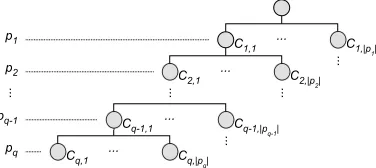
To address Requirement 3, we developed Paramorama, a prototype for the visual analysis of relationships between input parameter space and image-based outcomes. We use hierarchical clustering of the sampled parameters as starting point. As Figure 4 shows, and detailed below, the user interface consists of three views. First, a compact node-link representation provides an overview of the clustering hierarchy and serves as the primary navigation device (Figure 4(a)). Second, there is a refinement view for the analysis of user-selected areas of interest in the clustering hierarchy (Figure 4(b)). For this, we have developed a novel layout algorithm that provides perceptual support for investigating and comparing the image-based outcomes in the context of parameter space. Finally, we provide a reference image view to directly compare image-based outcomes with an input image (Figure 4(c)). Views are coordinated and are augmented with interactive features such as dynamic querying, user-defined parameter ordering, and user-specified tagging (Figure 4(d)–(j)).

Fig. 4. Visualization of parameter space for image analysis. (a) The overview shows sampled parameter values as a clustering hierarchy. (b) The refinement view shows scaled previews of the image-based outcomes for selected subtrees in the clustering hierarchy. (c) The reference image view superimposes the output that currently has the focus in the refinement view on a reference image. (d) Selected subtrees are highlighted in blue in the overview and (e) shown in distinct regions in the refinement view. (f) Users can specify a level in the clustering tree at which to position subtrees side-by-side in the refinement view. Further interactive features include: (g) brushing; tagging of (h) high-quality and (i) low-quality outcomes; and (j) filtering. The data set shown here was generated by sampling the parameter space of theIdentifyPrimaryObjectsmodule in CellProfiler for human HT29 cells (5 parameters, 4 samples each, yielding 1,024 outcomes). At this point the user has identified and tagged a number of high-quality outcomes where all cells have been detected (coded in green in the overview and detail view). The user has also tagged low-quality outcomes where all cells have not been detected (magenta). The distribution of green and magenta in the overview indicates which parts of parameter space to consider and which parts to disregard.

The numerical values that have been sampled have a natural order-ing. To respect this in a tabular representation, the tuplestican be ordered first forp1, then forp2, and so forth (like column sorting in a spreadsheet). The first column will contain|p1|blocks of identical values (with|p1|the cardinality ofp1). Theithblock will contain all tuples wherep1assumes theithvalue in its domain. For every block in the first column there will be|p2|blocks in column 2, and so on. Sorting tuples in this fashion produces a hierarchical arrangement of parameter values, which we took as the basis for defining a hierarchi-cal clustering on tuples. As shown in Figure 5, levelkin the hierarchy corresponds to parameterpk−1(the root, at level 1, contains all tuples).

We argue that hierarchical clustering offers a number of advantages over a tabular representation. A tree constructed as above respects the ordering of parameter domains. It also provides an accurate overview of all combinations of sampled values that is convenient to navigate. Instead of sorting columns in a table, the ordering of leaves can be changed intuitively by reordering parameters. As shown in Section 5, this enables users to identify robust combinations of parameters by looking for contiguous regions in the clustering hierarchy that correlate with high-quality outcomes. Finally, it has been shown that representing combinatorial data in a hierarchical fashion enables users to answer queries rapidly and intuitively across multiple data dimensions if provided with sufficient interactive capabilities [18].

Overview.This presents a structured overview of the sampled param-eter space by showing the clustering tree as a directed node-link dia-gram (see Figure 4(a)). The overview serves as the primary navigation aid with which users can select areas of interest in parameter space to

view in more detail. As users move the mouse cursor over nodes the subtree below the node in focus is highlighted in red. When a subtree is selected, the highlighting changes to blue and it is shown in more detail in the refinement view (see next section). Following standard practice, users can add multiple areas of interest by selecting further subtrees and remove selections by clicking on them a second time.

We based our choice of tree visualization on evidence suggesting that node-link representations are often better suited for showing and navigating hierarchical relationships than other representations such as icicle plots and treemaps [1, 12]. We considered different node-link layouts, including radial, but settled on a directed node-link diagram because it preserves the ordering of data values more explicitly by en-coding them in only one direction (top-to-bottom in our case). Another consideration was the aspect ratio and compactness of the representa-tion to maximize real-estate for the refinement view (see next secrepresenta-tion). To be space efficient, a radial layout requires an aspect ratio of 1:1. In practice, as here, visualization designers often wish to place compact overviews in an elongated area, which a directed layout utilizes better. We orient the node-link diagram from left to right to label nodes horizontally with their associated data values. Nodes are ordered from top to bottom as their associated values increase. Parameter values are encoded by a perceptually ordinal and colorblind safe color scale [3]. Luminance is high and saturation low to not clash with other color cues (see later sections). The directed layout also enables us to label each level of the tree with the parameter to which it corresponds.

p1 p2 ... pq−1 pq

t1 x1,1 x2,1 ... xq−1,1 xq,1

.. . .. . .. . .. . .. .

t|pq| x1,1 x2,1 ... xq−1,1 xq,|pq| t_|pq|+1 x1,1 x2,1 ... xq−1,2 xq,1

.. . .. . .. . .. . .. .

t_2|pq| x1,1 x2,1 ... xp−1,2 xq,|pq|

.. . .. . .. . .. . .. .

Table 1. Table-based representation of sampled parameters. Columns correspond to user-selected parameters. Each row represents a unique combination of sampled parameter values.

values. Each leaf node has a unique image-based outcome associated with it. To enable users to view and compare these results, we provide a refinement view (see Figure 4(b)). This view uses a novel layout algorithm to provide users with perceptual support for the analysis of the image-based outcomes produced by sets of parameter values. The algorithm has the following properties:

• It preserves the top-to-bottom ordering found in the overview, so there is a direct mapping between contiguous regions of pa-rameter space in the overview and their associated outputs in the detail view.

• It allows users to specify at which parameter level to position out-comes side-by-side. By being able to change this cutoff thresh-old, users can dynamically change the layout to suit their review and comparison requirements.

• It shows the outputs of the selected subtrees in adjacent, but visu-ally distinct areas, in the order they appear in the overview. This helps users to map each selected subtree in the overview with its representation in the detail view.

These properties of our algorithm assist users to understand how out-comes vary with respect to different parameter values.

Our layout algorithm is outlined below. For each subtreeT that has to be displayed, LAYOUTALLTREES() assigns an adjacent rectangular area with width proportional to the number of subtrees thatTcontains at the user-specified cutoff levelt. LAYOUTTREE() then lays out each subtreeT on the area it has been assigned by recursively traversing the nodes inT and nesting them in a manner inspired by treemaps [11]. Nodes at depthtare positioned side-by-side by dividing the width of the area assigned to a parent node between siblings. Other nodes are positioned top-to-bottom by division of the parent’s assigned height.

procedureLAYOUTALLTREES(LT,A,t) ⊲LTthe list of subtrees to layout

⊲Athe rectangular area available for layout ⊲tthe cutoff threshold at which to wrap subtrees

fori←1,LT.size()do

T ←LT.get(i)

c←c+T.getNumberSubtreesAtLevel(t)

end for

anchor←0

fori←1,LT.size()do

T ←LT.get(i)

c′←T.getNumberSubtreesAtLevel(t) A′.x←anchor

A′.y←A.getY()

A′.width←(c′/c)×A.getWidth() A′.height←A.getHeight() anchor←anchor+A′.getWidth()

returnLAYOUTTREE(T,A′,t)

end for end procedure p₁ p₂ p_q-1 p_q ...

C_1,1 C_1,|p

1|

C_2,1 C_2,|p

2|

...

...

... ...

...

C_q-1,1 C_q-1,|p

q-1|

...

C_q,1 C_q,|p

q|

...

...

Fig. 5. Hierarchical clustering of sampled parameters. Each level cor-responds to a user-selected parameter. The path from the root to each leaf represents a unique combination of sampled parameter values.

procedureLAYOUTTREE(T,A,t) ⊲T the subtree to layout

⊲Athe rectangular area available for layout ⊲tthe cutoff threshold at which to wrap subtrees

T.x←A.getX() T.y←A.getY() T.width←A.getWidth() T.height←A.getHeight() c←T.getChildCount()

fori←1,cdo

C←T.getChild(i)

ifC.level() =tthen

w←A.getWidth()/c A′.x←A.getX() + (i−1)×w A′.y←A.getY()

A′.width←w

A′.height←A.getHeight()

else

h←A.getHeight()/c A′.x←A.getX()

A′.y←A.getY() + (i−1)×h A′.width←A.getWidth() A′.height←h

end if

returnLAYOUTTREE(C,A′,t)

end for end procedure

As an example of the results that our algorithm produces, consider the following. In Figure 4(a), 11 subtrees of parameter space have been selected and these are mapped to 11 distinct regions in the refinement view in Figure 4(b). One of the subtrees contains 64 combinations of parameter values (Figure 4(d)). Of the corresponding outcomes 48 are visible and 16 have been suppressed (Figure 4(e)). Image-based outcomes are embedded directly in the layout. As noted, the cutoff thresholdtis user-specified and enables direct comparison of selected subtrees with respect to values assumed for the parameter with index equal tot. The value oftis shown in the overview by a vertical blue line that intersects the hierarchy at the specified level (Figure 4(f)).

The above pseudocode provides the gist of our layout algorithm. It is easily extended to add framed borders at each level of the hierarchy. It is also straightforward to extend the algorithm to assign leaf nodes equal height and to align all subtrees to the top of the display as we have done in our implementation. As with the overview, users can interact with the refinement view directly using their mouse cursor.

Our prototype enables users to load a reference image and shows this in the reference image view (see Figure 4(c)). When users move the mouse cursor over scaled images in the refinement view, the thumbnail that has the focus is overlaid on the reference image in this view. Users can also tear out the reference view to display it in a popup window that can be moved closer to a specific set of results in the refinement view.

Interaction.Our prototype consists of multiple coordinated views and it provides a number of ways to interact with the visualizations us-ing the widget panel or direct manipulation. This includes brushus-ing, tagging, parameter reordering, and filtering (see Figure 4(d)–(j)).

Brushing is used to highlight the current focus of a particular view in all other views. When the focus is on a single leaf, the image asso-ciated with that result is shown at a higher resolution in the reference image view. Color schemes are consistently applied across views: data values are encoded with a sequential color map, selections are high-lighted in blue (see Figure 4(d)) and the current focus in red (Fig-ure 4(g)). We show users the values of all parameters that correspond to their current focus in a text area below the refinement view. We found that traditional tooltips obscured too much of the display when a number of parameters and the values they assume have to be listed.

Our overview and refinement mechanism enables users to select subsets of the data and to view these in more detail while retaining context. To address Requirement 3, our prototype supports two high-level modes of selection, which are seamlessly integrated and do not require an explicit mode switch. The first facilitates drill-down and has already been discussed: users can select areas of interest in the overview, consider these in greater detail in the refinement view, and view individual results in even greater detail using the reference im-age view. To make selection less arduous, we also provide a facility to step through selections at a user-defined level in the clustering hier-archy. Using buttons or keyboard shortcuts, this tool selects the next unselected subtree and updates the refinement view accordingly. To aid selection, the overview distinguishes between nodes that have been considered (solid outlines) and those that have not (dashed outlines).

The second mode of selection was designed so that users can keep track of and relate high- and low-quality outcomes to parameter val-ues. This is achieved by tagging results as positive or negative using mouse clicks in the refinement view (see Figure 4(h) and (i)). Re-sults tagged as positive are color-coded in a green and those tagged as negative in magenta in both the overview and refinement view. These colors were chosen to be colorblind safe [3]. Users can toggle between tagging positive or negative using shortcut keys or the widget panel.

To change the levels of the clustering hierarchy, users can interac-tively reorder the parameters. The visualizations are automatically up-dated and all previous selections and tags remain intact. As mentioned before, users can specify the cutoff level at which selected subtrees are displayed side-by-side in the refinement view.

Finally, we offer users interactive filtering, also called dynamic querying [19], in two distinct modes. For parameter-based filtering users define an active range using the range sliders in the widget panel. Those parts of the clustering hierarchy that fall outside this range are filtered out in both the overview and refinement view. Users can spec-ify whether to gray out filtered data - as shown in Figure 4(j) - or to hide them completely. For filtering based on user-assigned tags, users can filter out any combination of positive, negative or untagged data using checkboxes in the widget panel. Again, these can be grayed out or hidden from view.

5 CASE STUDIES

A typical CellProfiler pipeline will contain modules do identify objects of interest. The nuclei are usually the first (primary) objects identified in a cellular image, as they form the basis for detection of other cellu-lar compartments. Therefore, optimizing the identification of nuclei is an essential part of a typical CellProfiler workflow. As noted in Sec-tion 4.1, a crucial module isIdentifyPrimaryObjects, normally used for nucleus detection. This module contains several settings which must be simultaneously optimized for effective nucleus identification.

We have chosen this module as the focus of our case studies to test the advantages of our new parameter optimization approach.

5.1 Novice user

Our first case study involves the detection of human HT29 colon cancer cells in images [22], which have an appearance similar to most human cell types used in biological experiments. The cells were stained with Hoechst 33342, a DNA stain which labels the nuclei. The time required to optimize parameters for aIdentifyPrimaryObjects

module depends on users’ experience and the complexity of objects in the image. Expert CellProfiler users, who have trained many novices, have found that for images comparable to HT29, a novice user can take upwards of an hour to converge on suitable parameter settings. An experienced user can achieve the task in approximately 10 minutes.

Parameter sampling. Our sampling plug-in automatically detected five parameters with continuous domains for the object detection module: threshold correction factor (p1), lower bound on threshold (p2), upper bound on threshold (p3), minimum diameter of objects (p4), and maximum diameter of objects (p5). Using the default values assigned to these parameters by CellProfiler as starting point, a range that deviates 25% above and below these values was specified, with four samples computed for each parameter. Our plug-in automatically generated 1,024 unique combinations of values, fed these into Cell-Profiler, and saved the detected nucleus outlines to disk. Setting up the sampling specifications took about a minute. Running the image analysis algorithms and saving the results to disk took approximately 29 minutes on a standard workstation with an Intel Core Due 2.8 GHz CPU with 8 GB RAM running Windows 7.

Visual analysis.We now describe how our technique enabled a novice CellProfiler user (first author) to systematically analyze those regions of parameter space that yielded low- and high-quality results. The user started with a clustering hierarchy based on the parameter order described above (p1–p5). The cutoff threshold for the refinement view was set to four to easily compare the nucleus outlines for adjacent outcomes in parameter space.

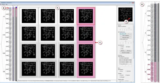
The user began by using the step-through selection feature for the hierarchy shown in the overview: the next previously unseen subtree at level three (see Figure 6(a)) was accessed with a single mouse click to show a 4×4 matrix of outcomes (Figure 6(b)). By comparing these images and by moving the mouse over individual images to super-impose them on the reference image, the user easily identified poor results and tagged these (Figure 6(c)). For the negatively tagged out-comes, note the missing outlines for the two nuclei just above the nu-cleus in the lower right (Figure 6(d)). The nested hierarchical rep-resentation in the refinement view enabled the user to save time by tagging entire subtrees, as opposed to tagging individual outcomes.

After identifying a few poor result sets the user suspected that these poor outcomes occurred when parameterp4=13, its highest sampled value. The user was able to quickly confirm this by moving p4 to the first level in the clustering hierarchy and by scanning all outcomes clustered under the last value forp4in the refinement view, none of which identified the two nuclei mentioned in the previous paragraph. All outcomes for this value of p4 were then tagged as negative, as shown in the bottom subtree of Figure 6(e). To reduce the complexity of subsequent analysis, the user next used the filtering facility of our prototype to hide all these negatively tagged outcomes.

Using an approach similar to the one described above, the user again starting scanning the parameter space by stepping through subtrees at level three of the clustering hierarchy. The user quickly saw that when

unfil-Fig. 6. Visualization of parameter space for human HT29 cells. (a) Nodes and leaves of the currently selected subtree are highlighted in blue, with the tagged nodes marked in magenta. (b) The overview panel showing a4×4grid of the selected outcomes (outlines of detected nuclei). (c) Outcomes in which two nuclei are missed are tagged as negative. (d) Reference image with outcome currently in focus overlaid. (e) Overview after parameters were reordered, a contiguous region has been tagged as low-quality.

tered values that were sampled for p4. At this point, the user could have accepted the parameter values and proceeded with automatically analyzing a large collection of similar images. Alternatively, it would have been possible to reapply the sampler to sample more finely within this region and to visually inspect the outcomes again.

Using the above approach, the novice user was able to identify in approximately 10 minutes a contiguous part of the parameter space that yields high-quality results. This is comparable to the time re-quired by an expert CellProfiler user to identify optimal parameter values using the conventional parameter optimization approach and, in our experience, far quicker than a novice taking this approach.

5.2 Expert user

We now describe a case study involving an expert user (second author). The user’s aim was to detect cell nuclei in human U2OS (osteoarcoma, or cancerous bone tumor) cells [21]. Two images that had respectively been treated with two drugs - Wortmannin and LY294002 - were con-sidered. They had been stained with DRAQ, a DNA stain, to label nuclei. Although very experienced with CellProfiler, the user had no prior hands-on experience with the sampling plug-in or the visualiza-tion prototype. The user took notes of the experience.

To compare the quality of the parameter values arrived at using our new parameter optimization approach with those identified with the conventional approach, the results were quantitatively assessed us-ing theZ′factor, which quantifies assay suitability for screening pur-poses [14]. For this measure,Z′=1.0 indicates optimal results, while

Z′>0.5 are of acceptable quality. As a control, the expert user also constructed and tuned two CellProfiler pipelines from scratch for com-parable Wortmannin and LY294002 treated images. The optimal set-tings identified using our approach scoredZ′=0.956 for Wortman-nin andZ′=0.902 for LY294002. Using the conventional approach, Wortmannin scoredZ′=0.900 and LY294002 scoredZ′=0.882. This indicates a slight, but meaningful, increase in the quality of results us-ing our approach. What is more, the quality of the results achieved with our approach scored higher than the prior best score obtained us-ing the conventional approach (Z′=0.940 for Wortmannin,Z′=0.900

for LY294002), which required many days of meticulous parameter tuning by an expert [5, 14].

We attribute the increase in quality to a more thorough analysis of parameter space. Using our approach, the expert was able to investigate and analyze 3,215 unique parameter combinations of each image. Identification of optimal parameter settings to accurately detect cell nuclei for the Wortmannin image took approximately four hours (performed first). The same task took approximately two hours for the LY294002 image, the time decreasing as the user became familiar with our tool. Far fewer parameter combinations were analyzed with the conventional approach (less than 20 for both images), so even though it took less time (approximately 30 minutes for each image) the time per combination was greater and the quality of results worse (see above). Thorough coverage of the parameter space would take days with the conventional approach, and would therefore be wholly impractical. The user’s notes also revealed that our approach made it possible to directly compare and analyze the relationships between multiple parameters in a way that is not possible using the conventional approach.

The above case studies suggest that our approach could lead to a paradigm shift in parameter optimization, resulting in higher quality outcomes. We find this very encouraging. To guide future designs, we plan to conduct further controlled experiments, involving novices and experts, where we will measure the time required to create satisfac-tory pipelines, the coverage of the parameter space explored, and the accuracy of results.

6 CONCLUSION

Fig. 7. (a) Reference image with the nucleus that is either detected or omitted. (b) Outcomes in which the nucleus is correctly detected and tagged as high-quality (shown in green). (c) Outcomes in which the nucleus is missed.

and to generate associated image-based outcomes. Second, we de-veloped a prototype visualization tool to allow users to analyze the relationships between parameter values and outcomes. To show how our approach supports more thorough parameter exploration and leads to higher quality results by reducing time cost and memory load -two case studies were presented.

Our sampling plug-in is publicly available in the developer’s ver-sion of CellProfiler to encourage a wider adoption of our approach [8]. Our visualization tool, called Paramorama, is available for free down-load at [17].

The work presented here addresses the primary issues highlighted by our requirements analysis. Our approach does have limitations, though. First, we offer users per-module-sampling and not an exhaus-tive search of parameter space. However, our interviews with experts and observations during case studies have indicated that users are typ-ically not interested in covering the entire parameter space (which is infinitely large). Based on their domain knowledge, they often have an idea of suitable parameter ranges and, in practice, are only interested in generating a handful of samples per parameter. Our approach en-ables them to consider the many possible interactions between param-eters in such regions of parameter space. This was prohibitively time-consuming with the conventional approach to parameter optimization. The interactions of parameters across modules is a related aspect that we do not currently address. Although this has not been flagged as a concern by users, we hypothesize that this is a result of their habit of approaching CellProfiler on a per-module basis. We argue that our overall strategy should apply to sampling multiple modules, but more work will be required for both sampling and visual analysis.

One way to address per-module-sampling is to incorporate metrics generated by image analysis algorithms. A simple example is the num-ber of objects detected. Users are likely to have a sense of values to expect and this could be used to rapidly filter parameter space. Metrics can also be used for the (semi-) automated arrangement of levels in the clustering hierarchy. Using such an approach, it might be possible to strike a balance between presenting outcomes based on quantitative features while capitalizing on the semantics that users associate with input parameters. Automation can be explored further, as noted in Section 1. If users could provide ground truth - by outlining cells, for

example - the outcomes could be filtered by classifiers built by ma-chine learning algorithms, but without requiring inordinate amounts of training time.

A second limitation relates to thumbnail-based exploration. Our work to date focuses on input images analyzed in biomedical labora-tories, which are typically a few hundred pixels squared. For this, the combination of a thumbnail-based refinement view plus native reso-lution detail-on-demand, as presented here, works well. Catering for very high resolution images, such as those in histopathology [23], and larger parameter spaces will require more work. One potential solu-tion is the deployment of our strategy on wall-sized gigapixel displays, which we are eager to test.

Our approach can be refined in a few more ways. We plan to extend our prototype so users can analyze the effect of the same parameters on multiple input images. The tagging mechanism can be made more general by enabling users to define custom categories. Allowing users to save final parameter choices in a format that can be read by CellPro-filer will streamline the implementation of our strategy. Finally, we are excited about the possibility of applying our approach to parameter-ized systems in other application domains. We have been approached by physicists working on a functional MRI (magnetic resonance imag-ing) simulation engine. The underlying challenge is almost identical to the problem addressed in this article: the analysis of the influence of input parameter settings on image-based output is very inefficient. Although we expect our approach to be applicable, we are keen to investigate which parts can be transferred effortlessly and what new design challenges will be raised.

ACKNOWLEDGMENTS

REFERENCES

[1] T. Barlow and P. Neville. A comparison of 2-D visualizations of hierar-chies. InProceedings of the IEEE Symposium on Information Visualiza-tion, pages 131–138, 2001.

[2] L. Bavoil, S. P. Callahan, P. J. Crossno, J. Freire, and H. T. Vo. VisTrails: enabling interactive multiple-view visualizations. InProceedings of the IEEE Conference on Visualization, pages 135–142, 2005.

[3] C. Brewer and M. Harrower, The Pennsylvania State University. Col-orBrewer website. http://www.colorbrewer2.org/. Last visited 20 June 2011.

[4] S. P. Callahan, J. Freire, E. Santos, C. E. Scheidegger, C. T. Silva, and H. T. Vo. Managing the evolution of dataflows with VisTrails. In Proceed-ings of the International Conference on Data Engineering Workshops, pages 71–75, 2006.

[5] A. E. Carpenter, T. R. Jones, M. R. Lampbrecht, C. Clarke, I. H. Kang, O. Friman, D. A. Guertin, J. H. Chang, R. A. Lindquist, J. Moffat, P. Gol-land, and D. M. Sabatini. CellProfiler: image analysis software for identi-fying and quantiidenti-fying cell phenotypes.Genome Biology, 7(R100), 2006. [6] R. Ferreira, B. Moon, J. Humphries, and A. Sussman. The virtual micro-scope. InProceedings of the American Medical Informatics Association Annual Fall Symposium, pages 449–453, 1997.

[7] D. Foulser. IRIS Explorer: a framework for investigation. SIGGRAPH Computer Graphics, 29:13–16, 1995.

[8] Imaging Platform, The Broad Institute of MIT and Harvard. CellProfiler, developer’s version. http://www.cellprofiler.org/developers.shtml. Last visited 20 June 2011.

[9] Imaging Platform, The Broad Institute of MIT and Harvard. CellPro-filer website, citations. http://www.cellproCellPro-filer.org/citations.shtml. Last visited 20 June 2011.

[10] T. J. Jankun-Kelly and K.-L. Ma. A spreadsheet interface for visualization exploration. InProceedings of the IEEE Conference on Visualization, pages 69–76, 2000.

[11] B. Johnson and B. Shneiderman. Treemaps: a space-filling approach to the visualization of hierarchical information. InProceedings of the IEEE Conference on Visualization, pages 284–291, 1991.

[12] A. Kobsa. User experiments with tree visualization systems. In Proceed-ings of the IEEE Symposium on Information Visualization, pages 9–16, 2004.

[13] M. R. Lamprecht, D. M. Sabatini, and A. E. Carpenter. CellProfiler: free, versatile software for automated biological image analysis. BioTech-niques, 42(1):71–75, 2007.

[14] D. J. Logan and A. E. Carpenter. Screening cellular feature measurements for image-based assay development.Journal of Biomolecular Screening, 15(7):840–846, 2010.

[15] K.-L. Ma. Image graphs – a novel approach to visual data exploration. InProceedings of the IEEE Conference on Visualization, pages 81–88, 1999.

[16] J. Marks, B. Andalman, P. A. Beardsley, W. Freeman, S. Gibson, J. Hod-gins, T. Kang, B. Mirtich, H. Pfister, W. Ruml, K. Ryall, J. Seims, and S. Shieber. Design galleries: a general approach to setting parameters for computer graphics and animation. InProceedings of the Conference on Computer Graphics and Interactive Techniques, pages 389–400, 1997. [17] A. J. Pretorius. Paramorama website. http://www.comp.leeds.ac.uk/

scsajp/applications/paramorama/. Last visited 20 June 2011.

[18] A. J. Pretorius and J. J. van Wijk. Visual inspection of multivariate graphs.

Computer Graphics Forum, 27(3):967–974, 2008.

[19] B. Shneiderman. Dynamic queries for visual information seeking.IEEE Software, 11(6):70–77, 1994.

[20] A. Squillacote. The ParaView Guide. Kitware, Inc, Clifton Park, NY, USA, third edition, 2008.

[21] The Broad Institute of MIT and Harvard. Broad Bioimage Benchmark Collection. http://www.broadinstitute.org/bbbc/sbs bioimage cnt.html. Last visited 20 June 2011.

[22] The Broad Institute of MIT and Harvard. Broad Bioim-age Benchmark Collection, Human HT29 colon cancer 1. http://www.broadinstitute.org/bbbc/human ht29 colon cancer 1.html. Last visited 20 June 2011.

[23] D. Treanor, N. Jordan-Owers, J. Hodrien, P. Quirke, and R. A. Rud-dle. Virtual reality powerwall versus conventional microscope for view-ing pathology slides: an experimental comparison. Histopathology, 55(3):294–300, 2009.

[24] L. Tweedie, B. Spence, H. Dawkes, and H. Su. The influence explorer. In

Proceedings of the Conference on Human Factors in Computing Systems, pages 129–130, 1995.

[25] L. Tweedie and R. Spence. The prosection matrix: a tool to support the interactive exploration of statistical models and data.Computational Statistics, 13(1):65–76, 1998.

[26] J. J. van Wijk and C. W. A. M. van Overveld. Preset based interaction with high dimensional parameter spaces. Data Visualization: The State of the Art, pages 391–406, 2003.