This is a repository copy of Team Theory and Person-by-Person Optimization with Binary
Decisions..
White Rose Research Online URL for this paper:
http://eprints.whiterose.ac.uk/89716/
Version: Accepted Version
Article:
Bauso, D. and Pesenti, R. (2012) Team Theory and Person-by-Person Optimization with
Binary Decisions. SIAM Journal on Control and Optimization (SICON), 50 (5). 3011 - 3028.
ISSN 0363-0129
https://doi.org/10.1137/090769533
[email protected] https://eprints.whiterose.ac.uk/
Reuse
Unless indicated otherwise, fulltext items are protected by copyright with all rights reserved. The copyright exception in section 29 of the Copyright, Designs and Patents Act 1988 allows the making of a single copy solely for the purpose of non-commercial research or private study within the limits of fair dealing. The publisher or other rights-holder may allow further reproduction and re-use of this version - refer to the White Rose Research Online record for this item. Where records identify the publisher as the copyright holder, users can verify any specific terms of use on the publisher’s website.
Takedown
If you consider content in White Rose Research Online to be in breach of UK law, please notify us by
TEAM THEORY AND
PERSON-BY-PERSON OPTIMIZATION
WITH BINARY DECISIONS
∗
D. BAUSO† AND R. PESENTI‡
Abstract. In this paper, we extend the notion of person by person optimization to binary decision spaces. The novelty of our approach is the adaptation to a dynamic team context of notions borrowed from the pseudo-boolean optimization field as completely local-global or unimodal functions and sub-modularity. We also generalize the concept of pbp optimization to the case where the Decision Makers (DMs) make decisions sequentially in groups ofm, we call itmbmoptimization. The main contribution are certain sufficient conditions, verifiable in polynomial time, under which a pbp or anmbm optimization algorithm leads to the team-optimum. As a second contribution, we present alocal andgreedy algorithm that allows the DMs to select a small neighborhood which guarantees them to behave as if they had complete information. As a last contribution, we also show that there exists a subclass of sub-modular team problems, recognizable in polynomial time, for which the convergence is guaranteed if the pbp algorithm is opportunely initialized.
Key words. team theory, person-by-person optimality, approximation algorithms
1. Introduction. Most fundamental results in team theory concern linear quadratic Gaussian problems or, in general, problems with continuous decision spaces, where the cost is somehow convex in the strategies and the information structure is a “nice” one (see, e.g., partial nested structures) [12, 16]. In such particular cases, it is well known that a simple solution idea consisting in a sequential optimization on the part of the Decision Makers (DMs), calledperson by person optimization (pbp), leads to the team-optimum [12], namely the argument minimizing the team objective function. In this paper, on the same line of [8, 9], we restrict our attention to boolean de-cision spaces. The novelty of our approach is the adaptation to a dynamic team con-text of notions borrowed frompseudo-boolean optimization [5], as Completely Local-Global (CLG) functions, Completely Unimodal (CU) functions (also known as acyclic unique sink orientations and abstract objective functions [15]) and sub-modular func-tions [6, 11].
Boolean decision spaces can be found in finite-alphabet control and in particular on-off control problems [2, 10], impulsively-controlled systems (activate the impulse or not) [7], or switching control (switches between active and passive modes) [17]. Boolean decisions are encountered in many applications as inventory with set up costs (reordering or not from a warehouse in order to meet a demand) [3, 4], distributed computer systems (processing or not the assigned task) [9], in air-conditioning systems control, in economics and finance (see, e.g., [5] and references therein).
As first contribution, we generalize the concept of pbp optimization to the case where the Decision Makers (DMs) make decisions sequentially in groups ofm, we call itmbmoptimization.
∗A conference version [1] of this paper has been published in the Proc. of the IEEE American
Control Conference, Seattle, Washington, USA, June 2008. Corresponding author D. Bauso Tel. +39-320-4648142. Research supported by MURST-PRIN 2007ZMZK5T “Decisional model for the design and the management of logistics networks characterized by high interoperability and informa-tion integrainforma-tion”.
†D. Bauso is with DINFO, Universit`a di Palermo, Italy[email protected] ‡R. Pesenti is with DMA, Universit`a “Ca’ Foscari” di Venezia, Italy[email protected]
The main contribution of this paper consists in providing certain sufficient condi-tions, verifiable in polynomial time, for the optimality of such pbp (respectivelymbm) optimization algorithms based on the knowledge of the agents’ states. Then we can frame our results in the literature on person by person algorithms in team theory, which has drawn the attention of the control audience since the ’70s (see, e.g., [12]).
A second contribution, which makes this paper to differ from the conference ver-sion [1], is thelocal andgreedy algorithm of Section 5. This algorithm allows the DMs to select a small neighborhood which guarantees them to behave as if they had com-plete information, i.e., they knew all the other agents’ states. “Small” neighborhood means that each DM is not required to communicate with all the other DMs but only with a restricted, possibly the minimal, number of them. “Local” means that the algorithm is implemented by the same DM who has to make a decision without any centralized mechanism. “Greedy” means that the DM who has to make a decision implements an iterative algorithm that at each iteration picks the smallest number of DMs whose state knowledge may be as informative as the knowledge of all the other agents’ states.
As a last contribution, we have paid special attention to problems with sub-modular team objective function (sub-modular team problems). Though sub-modularity alone does not guarantee the convergence of any pbp optimization algorithm, we show that there exists a special class of sub-modular team problems, recognizable in polyno-mial time, for which the convergence is guaranteed when the algorithm is opportunely initialized. This class is characterized by so-calledthreshold strategies.
This paper is organized as follows. In Section 2, we introduce some notions from team theory [12] and pseudo-boolean optimization [5]. In Section 3, we introduce the class of completely local-global functions and completely unimodal functions [6], and [11]. In Section 4, we address the mbm optimization. In Section 5, we present the greedy algorithm. In Section 6, we focus on sub-modular team problems. In Section 7 we provide numerical examples. Finally, in Section 8, we discuss how to extend the obtained results.
2. Definitions and Problem Statement. Consider a setN ofnDMs making decisionsxfrom a discrete hypercubeBn ={0,1}n. Decisions are made in order to
optimize a common team objective function, J(x) : Bn → Z, whereZ is the set of
integer numbers.
Assumption 2.1. The team objective function J(x) is injective and has the
following quadraticform
J(x) =
n
i=1 bixi+
i∈N
j∈N
aijxixj
(2.1)
withaij andbi integer (this causesJ(x) assuming only integer values).
The following definitions are slightly modified from [9].
Definition 2.1. (Team-optimum) A pointx∗ is a team-optimumif
x∗= arg min
x∈BnJ(x).
As the setBn is finite, a team optimum x∗ always exists. Furthermore, as J(x) is
injective, the team optimum is unique.
Definition 2.2. (pbp optimum)The pointx∗is a pbp optimumif for any DMi
the following condition holds
J(x∗i, x∗−i)< J(xi, x∗−i), ∀xi=x∗i
wherexi∈Bis the decision of DMiandx−i= (x1, . . . , xi−1, xi+1. . . , xn)T ∈Bn−1
is a vector collecting decisions of all other DMs. From the above definitions we have that a team-optimum always implies pbp optimality but not vice versa.
Let S any subset of N with m elements. We indicate this with S ⊆ N with
|S| =m, where|S|means cardinality of S. Let xS ∈Bm be a vector collecting the
decisions of all the DMs belonging to S, namely,xS = (xi : i∈S). Analogously, let
x−S ∈ Bn−m be a vector collecting the decisions of all the other DMs, x−S = (xi :
i∈N\S).
Definition 2.3. (mbmoptimum)The pointx∗ is an mbmoptimumif, for any
subsetS ⊆N with |S|=m, the following condition holds
J(x∗S, x∗−S)< J(xS, x∗−S), ∀xS =x∗S.
(2.3)
All the results stated in the following hold true for any value of the parameter m from 1 ton.
For each subsetS⊆N, we isolate from the team objective function (2.1) the only terms inxi withi∈S as follows
JS(x) =
i∈S
bixi+
i∈S
j∈N
aijxixj
and denote this last function as theS-projection ofJ(x). We observe that for anyS⊆N,
arg min ˜
xS∈{0,1}
J(˜xS, x−S) = arg min
˜
xS∈{0,1}
JS(˜xS, x−S).
Moreover, assume that DMs inS know the decisions of the only DMs in a neigh-borhood ΓS, with ΓS ⊆N\S.
Then, for each ΓS ⊆N\S we can also define as ΓS-approximation of JS(x) the
following function
ˆ
JS,ΓS(x) =
i∈S
bixi+
i∈S
j∈S∪ΓS
aijxixj+
i∈S
i∈N\(S∪ΓS)
aijxixˆj
(2.4)
where
ˆ xj=
1 ifaij>0
0 otherwise .
The above definition implies that ˆJS,ΓS(x) approximates from above JS(x), i.e.,
ˆ
JS,ΓS(x)≥JS(x) for allx∈B
n and all Γ
S⊆N\S.
Hereafter, for the sake of notation, we use the notationJi(x), ˆJi(x), and Γi, and
Γ{i}, in state ofJ{i}(x), ˆJ{i}(x), and Γ{i} respectively.
We are ready to generalize the concept of pbp strategy, introduced in [9] and [12], as follows.
Definition 2.4. A strategy µi : Bn−1 → B is pbp strict for DM i if, for any
x−i∈Bn−1, we have
µi(x−i) = arg min
˜
xi∈{0,1}
J(˜xi, x−i) = arg min
˜
xi∈{0,1}
A strategy µˆi : Bn−1 → B is a Γi-approximation, for some Γi ⊆ N \ {i}, of a pbp
strict strategyµi(x−i)if, for anyx−i∈Bn−1, we have
ˆ
µi(x−i) = arg min
˜
xi∈{0,1}
ˆ
Ji,Γi(˜xi, x−i).
AsJ(x) is injective, the above equations have a unique solution. Then, under a strict pbp strategy µi(·), DM ichanges decision from zero to one or vice versa only
if such a change lets the{i}-projectionJi(·,·), and the team objective functionJ(·,·)
as well, decrease for fixed decisions of all other DMsj=i.
We can repeat the same argument for the Γi-approximate strict pbp strategy ˆµi(·)
with respect to the Γi-approximation ˆJi,Γi(·,·).
Definition 2.5. A strategyµS :Bn−m→Bmis mbmstrictfor DMs inS where
S⊆N with cardinality |S|=m if, for anyx−S ∈Bn−m, we have
µS(x−S) = arg min
˜
xS∈Bm
J(˜xS, x−S) = arg min
˜
xS∈Bm
JS(˜xS, x−S).
A strategyµˆS :Bn−m→Bm is aΓS-approximation, for someΓS⊆N\S, of ambm
strict strategyµS(x−S)if, for any x−S∈Bn−m, we have
ˆ
µS(x−S) = arg min
˜
xS∈{0,1}
ˆ
JS,ΓS(˜xS, x−S).
The above definition of strict mbm strategy has the following geometric inter-pretation. For any x∈ Bn and S ⊆ N, denote by ΠS(x) as the the corresponding
m-dimensional face {x˜ = (˜xS, x−S) ∈ Bn : x−S fixed} of hypercube Bn. Then, a
strict mbm strategy means that either (xS, x−S) is the optimal vertex in ΠS(x) or
the DMs inS coordinate their decisions to find an optimal vertex in ΠS(x).
With the above definitions in mind, we callpbp optimization algorithm, any al-gorithm that returns a sequence of decisions x(0) → x(1) → . . . where, for each iterationt, we denote byx(t) ={x1(t). . . xn(t)}andxi(t) the vector of decisions and
the decision of DMirespectively. We also require that each decisionx(t) is obtained from x(t−1) by a unilateral improvement on the part of a single DM i=σ(t), i.e., x(t) = [µi(x−i(t−1)), x−i(t−1)], whereσ:N→N, is a periodic surjective function,
with periodn, that returns a DM for each iterationt. For instance,σ(1) = 2,σ(2) = 5 . . .means that at iteration 1, DM 2 plays the strict pbp strategy for fixed decisions of all other DMs, and similarly for DM 5 at iteration 2. We define anmbmoptimization algorithm in a similar manner. Here, the functionσbecomesσ:N→ Q, with period |Q|, whereQis the set of all subsetsS ⊆N with|S|=m, and the vector of decisions at iterationt becomes x(t) = [µS(x−S(t−1)), x−S(t−1)]. We define an algorithm
approximate when it uses approximate strategies ˆµi(·) or ˆµS(·).
We can now state the problem of interest.
Problem 1. Find conditions under which any pbp (respectivelymbm)
optimiza-tion algorithm converges to the team-optimum. Furthermore, design local informaoptimiza-tion mechanisms under which approximate algorithms return the same decisions as in the complete information case.
Throughout the paper, convergence means “from any genericx(0)”, unless spec-ified differently.
Remark 2.1. Any strict pbp (respectively mbm) optimization algorithm
con-verges to a pbp (mbm) optimumx∗pbp (respectively x∗mbm) in a finite number of itera-tions. Actually, the setBn is finite and at each iterationt of the algorithm the value
There is a vast literature on functionsf(x) :Bn →Z that map from a discrete
hypercubeBn to the ordered fieldZof integer numbers. They are usually referred to
aspseudo-boolean functions [5].
In the following, we recall some notions and optimality conditions in the context of pseudo-boolean optimization that we use to prepare and motivate the results of the next sections.
Let us now associate to a binary vectorx∈Bn its neighborhoodNr(x) ofradius
r, defined as Nr(x) = {y : ρH(x, y) ≤ r}, where ρH(x, y) denotes the Hamming
distance of the vectorsxandy, defined as the number of components in which these two vectors differ. According to this definition, the neighborhood of radiusnof each x∈Bn is equal toBn, that isNn(x) =Bn.
A vector x is a local minimum of a pseudo-boolean f(.) if f(y) ≥ f(x) for all neighboring vectorsy∈N1(x). It is aglobal minimum iff(y)≥f(x) for all vectors y∈Bn.
Local minima can be determined by means of local search algorithms. In par-ticular, [6] defines as a single switch algorithm any algorithm that at each iteration proceeds to a better neighbor of the current iterate, by changing one coordinate at a time, until a local optimum is found. Similarly, they define as a multiple switch algorithm of ordermany algorithm that at each iteration proceeds to a next better iterate that differs from the current vertex in at mostmcoordinates.
Remark 2.2. The following statements hold true:
i) The team objective functionJ(x) is a pseudo-boolean function.
ii) Any pbp (respectively mbm) optimum is a local optimum in a neighborhood of radius one (respectively m).
iii) The team-optimum is a global optimum.
iv) Strict pbp (respectivelymbm) strategies are single (respectively multiple) switch algorithms.
There is a large variety of techniques applied in the literature for solving problems that can be modelled by quadratic pseudo-Boolean functions optimization. As this last problem is NP-hard, many of the published algorithms are implicitly enumerative. However, specialized optimization algorithms have been developed for increasing or decreasing pseudo-Boolean functions.
We can associate to a pseudo-boolean function its first orderithderivative
∂f ∂xi
(x) =f(x1, . . . , xi−1,1, xi+1, . . . , xn)−f(x1, . . . , xi−1,0, xi+1, . . . , xn),
which will be used later on. If f(.) is injective, ∂x∂f
i(x) = 0 for all x ∈
Bn, for all
i∈N. Let us finally introduce the following operation.
Definition 2.6. Given a function f : Bn →R, for any subset S ⊆ N, define
restrictionoff intoS,RSf(x) :Bn →Rthe function RSf(x) =
i∈S
bi+
i∈S
j∈S
aij+
k∈S
i∈S
aikxk.
The above definition has the following geometric interpretation. Consider the face ΠS(x) :{x= (xS, x−S)∈Bn : x−S fixed} ofBn and extract two pointsx= (1, x−S)
and x= (0, x−S) from it. Note that, for fixedx−S, inx all DMsi ∈ S set xi = 1
while inxall DMsi∈S setxi= 0. Then, the restriction is the differenceJ(x)−J(x)
of the team objective function computed on the two points. Also, note that for a singleton,S ={i}, thenRSf(x) = ∂x∂f
3. Person by Person Optimization. In this section, we present sufficient conditions, verifiable in polynomial time, for the convergence of any pbp algorithm to the team-optimum.
Definition 3.1. (CLG-functions [11]) An injective function f : Bn → Z is
Completely Local-Global(CLG) if inBn there is a unique local minimum.
Lemma 3.1. Any pbp optimization algorithm guarantees convergence to the
team-optimum x∗ if and only if J(x)is a CLG-function.
Proof. (sufficiency) IfJ(.) is a CLG-function then there is a unique pbp optimum which is also team-optimum. Any pbp optimization algorithm guarantees convergence to it.
(necessity) IfJ(.) is not a CLG-function then there is a second pbp optimum ¯xwhich is not team-optimum. Any pbp optimization algorithm starting at ¯xcannot deviate from it and therefore does not reach the global optimum.
The class of CLG-functions includes the class of completely unimodal functions.
Definition 3.2. (CU-functions) An injective functionf :Bn →ZisCompletely
Unimodal(CU) iff has a unique local minimum on every face ofBn.
We can derive the following corollary from the above lemma.
Corollary 3.1. Any pbp optimization algorithm converges to the team-optimum
x∗ ifJ(x) is a CU-function.
To the best of author’s knowledge, recognizing CU-functions or CLG-functions is, in general, a difficult task. Actually, it involves an exponential number of conditions as shown next. Furthermore, even iff is a CLG or CU-function, strict pbp strategies may converge in exponential time.
To see why completely unimodality involves an exponential number of conditions consider that for the existence of two local minima on a 2-face containingxi and xj,
it must hold
∂f(x) ∂xi
xj=0
· ∂f(x)
∂xi
xj=1
<0 (3.1)
∂f(x) ∂xj
xi=0
· ∂f(x)
∂xj
xi=1
<0. (3.2)
Then forf to be CU it is necessary that, on each 2-face and for all x, the above conditions are not satisfied, which implies an exponential number of verifications.
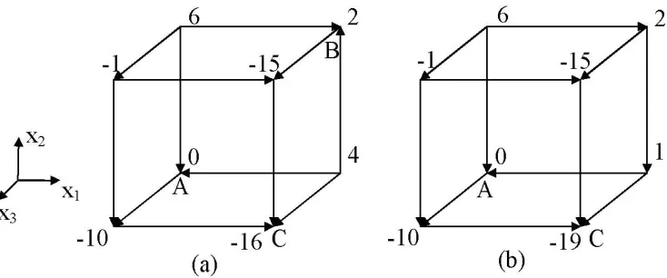
Example 3.1. Consider the set B3 = {0,1}3 and the team objective function J(x) :B3 →Z, taking on the values displayed in Fig. 3.1.a. The explicit expression
of the functionJ according to the formula (2.1) is
J(x) = 4x21+ 4x22−8x1x2+ 2x2
J(x1,x2)
−10x3−10x1x3+ 3x2x3,
where we denote by J(x1, x2) the function obtained considering terms only in x1
andx2. In Fig. 3.1.a, the oriented arcs indicate the decreasing directions for the team
objective function J(x). Function J(x) is a CLG-function as it has a unique local (global) minimum inB3 which is x= (1,0,1) (point C in the figure). However note
thatJ(x1, x2)is not a CLG-function as it has two local minima inB2. For instance,
Fig. 3.1.Unit 3-dimensional cubes: oriented arcs indicate decreasing directions forJ(x)when (a)J(x)is CLG-function or (b)J(x)is CU-function. Solutionsx= (0,0,0)andx= (1,1,0)(point
AandBin (a)) are two local minima for the 2-face x1-x2 withx3= 0. In both cases, the global
minimum isx= (1,0,1)(pointC).
function Jˆ(x) : B3 → Z, taking on the values displayed in Fig. 3.1.b. The explicit
expression is
ˆ
J(x) =x21+ 4x22−5x1x2+ 2x2
ˆ
J(x1,x2)
−10x3−10x1x3+ 3x2x3,
where againJˆ(x1, x2)is obtained considering terms only in x1 andx2. In Fig. 3.1.b,
the unique global minimum is againx= (1,0,1)(point Cin the figure) but differently from before function J(x) is a CU-function in B3 as it has a unique local minimum
on each 2-face. In correspondence to such a situation we also have that Jˆ(x1, x2) is
a CLG-function on B2 as it has a unique local minimum in B2 (see the 2-face x1-x2
withx3= 0which has a local minimum in x= (0,0,0) (point A)).
A special case of completely unimodality is when f(.) is monotonic along any single direction, which corresponds to being both left hand side of (3.1) and (3.2) positive. Now,f(.) is monotonic along any single direction, when for alli= 1. . . , n, one of the following mutually exclusive conditions holds true
max
x∈Bn
∂J(x) ∂xi
<0 (3.3)
min
x∈Bn
∂J(x) ∂xi
>0. (3.4)
We can specialize Corollary 3.1 to such a particular case.
Lemma 3.2. (Sufficient conditions) If the team objective function J(x) is such
that, for alli∈N, either (3.3) or (3.4) hold, then 1. the team optimum is
x∗i = 1 ifmaxx∈Bn
∂J(x)
∂xi <0
0 ifminx∈Bn ∂J(x)
∂xi >0
3. any pbp optimization algorithm converges to the team optimumx∗in at most
niterations.
Proof. Item 3 is straightforward from item 2. To prove item 1 and 2 consider that if max∂J∂x(x)
i <0, then
∂J(x)
∂xi <0 for allx. Analogously, if min
∂J(x)
∂xi >0 then
∂J(x)
∂xi >0 for allx.
Let us finally observe that verifying whether (3.3) or (3.4) holds is easy (poly-nomial inn), as we just have to find the maxima, respectively the minima, of the n functions ∂J∂x(x)
i linear inx∈
Bn.
4. Generalization to mbm Optimization. Let us now generalize the results established in the preceding section to the case where DMs make decisions sequentially in groups ofm.
Theorem 4.1. (Sufficient conditions) Letx∗=1be an(m−1)b(m−1)optimum,
if the team objective functionJ(.)is such that for all S⊆N with|S|=m it holds
max
x∈BnRSJ(x)<0
(4.1)
then
1. x∗ is the team-optimum
2. x∗ is also the uniquembm optimum,
3. any mbmoptimization algorithm converges to the team-optimum x∗.
Proof. Item 3 is straightforward from item 2. To prove item 1 and 2, let us assume by contradiction that there exists a team optimum valuex∗=1. LetV ={i:x∗i = 0}. The cardinality ofV cannot be greater than or equal tom. Indeed considerS ⊆V with|S|=m, sinceRSJ(x∗)<0 impliesJ(x◦)< J(x∗), wherex◦ ∈Bn differs from
x∗ only for the components inS, i.e., x◦i = 0 ifi∈V \S,x◦i = 1 otherwise. Thenx∗ should be within an Hamming distance strictly less thanmfrom1, but this situation cannot occur since1by definition is optimum within its neighborhood of radiusm−1.
Example 4.1. Consider the team objective functionJ(x) =x1+x2−3x3−5x1x2+
x1x3+x2x3.The solution x∗ =1is a pbp optimum as, for all i,bi+k=iaik <0.
Since for all S, with |S| = 2 condition (4.1) holds (for i = 1 and j = 2, we have
b1+b2+a12+ maxx∈Bn(a13+a23)x3=−1), thenx∗=1is also team-optimum.
Remark 4.1. In the above lemma, the assumption x∗ = 1 is without loss of
generality. Actually, if the team problem has a unique team optimumx∗=1then the
following transformation can be applied to the decision space such that the new team optimum is xˆ∗= 1:
ˆ xi=
xi ifx∗i = 1
1−xi it x∗i = 0.
(4.2)
Let us finally observe that verifying whether (4.1) holds is, for fixedm, polynomial innalthough exponential inm, as we just have to find the maxima of then
m
functions
RSJ(x) linear inx∈Bn.
5. A greedy algorithm to find a small set Γσ(t). Assume that at time t DMσ(t) may choose its neighborhood Γσ(t). In this context, we present alocal
which Γi-approximate, respectively ΓS-approximate, strategies ˆµi(·) or ˆµS(·)
repro-duce exactly the behavior of strict pbp strategies ˆµi(·), ormbmstrategies ˆµS(·).
Given an initial pointx(0), consider the pbp optimization algorithm. Leti=σ(t) be the DM picked by the algorithm at stept. The DMistrategy provides the following result
xi(t) =
1 if ∂Ji
∂x
x(t−1)=bi+
j∈Naijxj(t−1)≤0
0 otherwise .
Here note that the value ofxi(t) depends only on the sign of ∂J∂xi
x(t−1)and not on its exact value. In general, the strategyµi(x−i(t−1)) may not need to know the values
of all thexj(t−1), forj∈N to determine the sign of ∂J∂xi
x(t−1)and, hence, to return the value of xi(t). As a consequence, an approximate pbp optimization algorithm
certainly converges tox∗pbpif, at each stept, the DMichooses a Γi(t) so that the sign
of ∂Jˆi,Γi
∂x is equal to the sign of ∂Ji
∂x and, hence, ˆµi(x−i(t−1)) =µi(x−i(t−1)).
In particular, the DMimay choose the set Γi(t) by iteratively solving the following
problem:
z= min
j∈N
yj
bi+
j∈Di
aijxj(t−1) +
j∈A+
i
aij(1−yj) +
j∈A−
i
aijyj ≤0
(5.1)
yj ∈ {0,1} ∀j∈N
where: the binary variablesyj, forj∈N, are defined as follows
yj=
1 ifj∈Γi(t)
0 otherwise ;
the set Di is the set of DMs whose values xj(t−1) are known in advance by DM
i; finally, the sets A+i and A−i are such that A+i = {j ∈ N \Di : aij > 0} and
A−i ={j∈N\Di:aij ≤0}.
Lety∗ ={yj∗:j ∈N} be an optimal solution (if it exists) for (5.1) and Γi(t) = {j∈N :y∗
j = 1} ∪Dithe corresponding neighborhood ofi. Problem (5.1) determines
a minimal set Γi(t) of DMs that must be considered by DMito be sure that ˆµi(x−i(t−
1)) =µi(x−i(t−1)) = 1, given the knowledge ofxj(t−1), forj∈Di. Indeed, if the
following conditions hold
xj(t−1) = 0,for eachj such thatyj∗= 1 andj ∈A+i ,
xj(t−1) = 1,for eachj such thatyj∗= 1 andj ∈A
− i , (5.2) then ∂Ji ∂x
x(t−1)
≤bi+
j∈Di
aijxj(t−1) +
j∈A+i
aij(1−yj∗) +
j∈A−i
aijy∗j =
∂Jˆi,Γi
∂x
x(t−1)
≤0.
Now, let us observe that three situations may occur:
i) problem (5.1) has no feasible solution, that is Γi(t) =Di;
iii) problem (5.1) has an optimal solutiony∗ and conditions (5.2) do not hold. If situation i) occurs, then both ∂Jˆi,Γi
∂x
x(t−1) and
∂Ji
∂x
x(t−1) are strictly positive. Hence, ˆµi(x−i(t−1)) =µi(x−i(t−1)) = 0.
If situation ii) occurs, then both ∂Jˆi,Γi
∂x
x(t−1) and
∂Ji
∂x
x(t−1) are non positive. Hence, ˆµi(x−i(t−1)) =µi(x−i(t−1)) = 1.
Differently, if situation iii) occurs, DM i cannot conclude that ∂Jˆi,Γi
∂x
x(t−1) =
∂Ji
∂x
x(t−1). In this last situation, DM i must enlarge the set Di by including even the indexes of DMs whose values xj(t−1) have been interrogated by DMi before
realizing that conditions (5.2) do not hold. Then, DMidetermines a further tentative set Γi(t) by solving (5.1) again.
The above procedure is iterated, starting fromDi=∅, until either situationi) or
ii) occurs. At each iteration the cardinality ofDiincreases at least by one unit. Then,
in the worst case, after at maximum n−1 iterations, the procedure stops as Γi(t)
has become equal toN \ {i} and hence ∂Jˆi,Γi
∂x
x(t−1)=
∂Jˆi,N\{i}
∂x
x(t−1)=
∂Ji
∂x
x(t−1)
as ˆJi,N\{i} =Ji.
Let us finally observe that Problem (5.1) can be solved in polynomial time. In-deed, rewrite Problem (5.1) as
z= min
j∈N
yj
j∈A+i∪A
−
i
ˆ
aijyj ≥ˆbi
(5.3)
yj∈ {0,1} ∀j∈N
where ˆbi=bi+j∈Diaijxj(t−1) +
j∈A+i aij and ˆaij =
aij ifaij∈A+i −aij ifaij∈A−i
.
Problem (5.3) is a relaxed (polynomial time) version of the change making prob-lem [14] and its optimal solution can be trivially determined. Initially, re-denominate the DMs inA+i ∪A−i so that ˆaij ≥ˆaik ifj < k, then set
yj∗= 0 if
k∈A+i∪A
−
i, k<jˆaik ≥
ˆ bi
1 otherwise .
Similarly to (5.1), the DMsi∈S may determine whetherRSf(x)≤0 choosing
a set ΓS(t) by iteratively solving the following problem:
z= min
j∈N\S
yj
i∈S
bi+
i∈S
j∈S
aij+
i∈S
k∈(N\S)∩DS
aikxk(t−1) +
+
i∈S
k∈(N\S)∩A+S
aik(1−yj) +
i∈S
k∈(N\S)∩A−S
aijyj ≤0
(5.4)
where: the binary variablesyj, forj∈N\S, are defined as follows
yj=
1 ifj∈ΓS(t)
0 otherwise ;
the setDS is the set of DMs whose values xj(t−1) are known in advance by DMs
i∈S; finally, the setsA+S and A−S are such that A+S ={j ∈N \DS : aij >0} and
A−S ={j∈N\DS :aij ≤0}.
A little more difficult is for the DMsi∈S to choose a ΓS(t) so that ˆµi(x−S(t−
1)) =µi(x−S(t−1)).
Actually,x∗
S =µi(x−S(t−1)) if, for all ˜xS∈Bm,
i∈S
bi(x∗i −x˜i) +
i∈S
j∈S
aij(x∗ix
∗
j−˜xix˜j) +
i∈S
k∈N\S
aik(x∗i −x˜i)xk(t−1)≤0
Then, the DMs i ∈ S may determine whether a tentative ˆxS ∈Bm is equal to
µi(x−S(t−1)) choosing a set ΓS(t) by iteratively solving the following problem:
z= min
j∈N\S
yj
i∈S
bi(ˆxi−x˜i) +
i∈S
j∈S
aij(ˆxixˆj−x˜ix˜j) +
i∈S
k∈(N\S)∩DS
aik(ˆxi−x˜i)xk(t−1) +
+
i∈S
k∈(N\S)∩A+S
aik(ˆxi−x˜i)(1−yj) +
(5.5)
+
i∈S
k∈(N\S)∩A−S
aij(ˆxi−x˜i)yj ≤0 ∀x˜S ∈Bm
yj∈ {0,1} ∀j∈N
where the binary variablesyj, forj∈N\S, and the setsDS,A+S andA−S are defined
as for (5.4).
Now, let us observe that three situations may occur:
i) problem (5.5) has no feasible solution;
ii) problem (5.5) has an optimal solutiony∗ and conditions (5.2) hold;
iii) problem (5.5) has an optimal solutiony∗ and conditions (5.2) do not hold. If situation i) occurs, then ˆxS is not µi(x−S(t−1)), a different xS ∈ Bm must be
considered as tentativeµi(x−S(t−1)).
If situationii) occurs, then ˆxS=µi(x−S(t−1)).
Differently, if situation iii) occurs, DMs i ∈ S cannot conclude neither ˆxS =
µi(x−S(t−1)) nor ˆxS =µi(x−S(t−1)). In this situation, DMsi ∈S must enlarge
the set DS by including even the indexes of DMs whose values xj(t−1) have been
interrogated by DM i∈ S before realizing that conditions (5.2) do not hold. Then, DMsi∈S solves (5.5) again.
The above procedure is iterated, starting from DS =∅, until either situation i)
or ii) occurs. At each iteration the cardinality ofDS increases at least by one unit.
Then, in the worst case, after at maximum n−m iterations, the procedure stops as ΓS(t) has become equal toN\S.
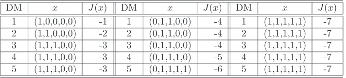
Table 6.1
Sequence of DMs’ decisions: blocks on the left, middle and right describe the first, second and third round of optimization.
DM x J(x) DM x J(x) DM x J(x) 1 (1,0,0,0,0) -1 1 (0,1,1,0,0) -4 1 (1,1,1,1,1) -7 2 (1,1,0,0,0) -2 2 (0,1,1,0,0) -4 2 (1,1,1,1,1) -7 3 (1,1,1,0,0) -3 3 (0,1,1,0,0) -4 3 (1,1,1,1,1) -7 4 (1,1,1,0,0) -3 4 (0,1,1,1,0) -5 4 (1,1,1,1,1) -7 5 (1,1,1,0,0) -3 5 (0,1,1,1,1) -6 5 (1,1,1,1,1) -7
recognize in polynomial time a special class of sub-modular team problems, which do not meet the aforementioned conditions and for which the convergence is guaranteed at least when the pbp algorithm is opportunely initialized. This class is characterized by so-calledthreshold strategies.
Let us callsub-modular team problems, all team problems with sub-modular team objective function. From [5], we remind from that i) a pseudo-Boolean functionf(.) is sub-modular if f(v) +f(w) ≤ f(vw) +f(v∨w) ii) a quadratic pseudo-Boolean function f(.) is submodular iff its quadratic terms are nonpositive. However, from the following example, it is apparent that sub-modularity alone does not guarantee the convergence of any pbp optimization algorithm.
Example 6.1. Consider the sub-modular team objective function J(x) = x1+
x2−3x1x2 and take x(0) = (0,0). The team optimum is (1,1) but observe that at
iteration 1, no DM alone benefits from changing its decision from 0 to 1. Hence the pbp optimization algorithm starts and terminates in (0,0).
We can generalize the above reasoning to show that sub-modularity alone does not guarantee the convergence of anymbmoptimization algorithm. On this purpose, note that if the team objective function is sub-modular, then condition (4.1) reduces to
i∈S
bi+
i∈S
j∈S
aij<0, for allS, with|S|=m.
(6.1)
We derive the above result by reminding that all quadratic terms are nonpositive and therefore maxxk=i,j(aik+ajk)xk ≤0 with the equality verified inx= 0.
Example 6.2. Consider the sub-modular team objective function J(x) = 2x1+
2x2+ 2x3−3x1x2−3x1x3−3x2x3and takex(0) = (0,0). The team optimum is again (1,1) but observe that at iteration 1, no pairs i and j of DMs alone benefits from changing their decisions from 0 to 1. Note that condition (6.1) for m = 2 becomes
bi+bj+aij <0 and there is no pair i and j that satisfies such a condition. Hence
the mbmoptimization algorithm starts and terminates in (0,0).
6.1. A Special Class with Threshold Strategies. Threshold strategy means that a DM i choosesxi = 1 if and only if at least other li DMs do the same. The
following simple example shows that when DMs have threshold strategies the team objective function is sub-modular. The team objective function is as in (2.1). We say that DMi has a threshold strategy with thresholdli =k, if its strict pbp strategy is
µi(x−i) =
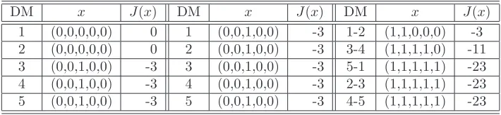
Table 6.2
Sequence of decisions: first and second round of pbp optimization (left and middle blocks), 2b2 optimization (right block).
DM x J(x) DM x J(x) DM x J(x) 1 (0,0,0,0,0) 0 1 (0,0,1,0,0) -3 1-2 (1,1,0,0,0) -3 2 (0,0,0,0,0) 0 2 (0,0,1,0,0) -3 3-4 (1,1,1,1,0) -11 3 (0,0,1,0,0) -3 3 (0,0,1,0,0) -3 5-1 (1,1,1,1,1) -23 4 (0,0,1,0,0) -3 4 (0,0,1,0,0) -3 2-3 (1,1,1,1,1) -23 5 (0,0,1,0,0) -3 5 (0,0,1,0,0) -3 4-5 (1,1,1,1,1) -23
Lemma 6.1. If all DMs have threshold strategies then the team objective function
J(x)must be sub-modular.
Proof. Observe that DM i has a threshold strategy withli = k. Denote by S(k) the set of all subsets ofN, which do not contain DMiand have cardinality less thank. Now, for a generic subsetS ∈ S(k), takex−i such thatxj = 1 for allj ∈S
and xj = 0 for allj ∈ N\(S{i}) and observe that from (6.2) it must hold that
µi(x−i) = 0. But this means that the following condition holds true
bi+
j∈S
aij≥0for allS∈ S(k).
(6.3)
Repeat the same reasoning considering a generic subsetS ⊆N\ S(k), and take x−i
such thatxj = 1 for allj∈S withj=iandxj= 0 for allj ∈N\S. Observe that
from (6.2) it must hold thatµi(x−i) = 1 which implies that the following condition
hold true
bi+
j∈S
aij<0for allS ⊆N\ S(k).
(6.4)
Now, consider two setsS1∈ S(k) with|S1|=k−1 andS2=S1∪ {j} ∈N\ S(k). Observe thatS2 has cardinality|S2|=kas it is obtained fromS1by adding a single DMj. We complete the proof by observing that for (6.3) and (6.4) to be valid it must be aij <0 for all iand j. Then J(.) has all quadratic terms negative which proves
thatJ(.) is sub-modular.
This special class of sub-modular team problems is interesting as i) threshold structures can be recognized in polynomial time and ii) any pbp optimization algo-rithm initialized atx(0) =1converges to the team-optimumx∗, in general different from1, as established in the following theorem.
Theorem 6.1. There exists a polynomial algorithm that verifies conditions (6.3)
and (6.4) inO(n2logn). In case of positive answer, any pbp optimization algorithm
initialized atx(0) =1converges to the team-optimum.
Proof. (Complexity) Given a DM i, consider all DMs except i in the order σ(1), . . . , σ(n) withaiσ(1) ≤. . . ≤aiσ(n). We remind here that the ordering process
has a complexityO(nlogn). Now, conditions (6.3) and (6.4) are verified if and only ifbi+aiσ(1)+. . .+aiσ(k−1) ≥0 andbi+aiσ(n−k)+. . .+aiσ(n) <0. We can limit ourselves to verify the latter two conditions for any possible value of the threshold li from 1 to n. Such a procedure is carried out via a dicotomic search and has a
and as O(nlogn) dominates (is always greater than) O(logn) the total complexity simply reduces to the cost of the ordering processO(nlogn). We conclude our proof by noticing that the ordering process must be repeatedn times (one for all DM i) and therefore the resulting complexity isO(n2logn).
(Convergence of pbp) Assume DMs ordered by increasing thresholds, i.e., l1 ≤ . . . ≤ ln. Starting at x(0) = 1 any pbp optimization algorithm converges to the
pbp optimum nearest to1(in terms of Hamming distance), call it ˆx. In other words ˆ
x= arg min{x−1: xis pbp-opt.}. We must show that ˆxis also the team-optimum. To prove this fact corresponds to proving that, if there exists a second pbp optimum, call it ˜x, it must hold
J(ˆx)−J(˜x) =RSJ(˜x) =
=
i∈S
bi+
i∈S
j∈S
aij+
r∈S
i∈S
airx˜r≤0,
where S is the set of components which are zero in ˜xand one in ˆx. Now note that
i∈S
j∈Saij+r∈S
i∈Sairx˜r=i∈S
r∈Nairxˆrand therefore we can rewrite
the above inequality as
J(ˆx)−J(˜x) =
i∈S
(bi+
r∈N
airxˆr) =
i∈S
(bi+
r∈S¯
air)≤0,
(6.5)
where we denote by ¯S the set of components which are one in ˆx. Then we need to prove the validity of (6.5). Now, note that if DMs are ordered by increasing thresholds, it must hold ˜x≤xˆ component-wise. Hence, as ˆxis a pbp optimum then eachi∈S has thresholdli<xˆ−0=xˆwhich in turns implies thati∈S(bi+
r∈S¯air)≤0
and therefore (6.5) hold true.
Remark 6.1. Threshold strategies simplify the search for a small
neighbor-hoodΓσ(t). DMs may implement a random selection of neighbors based only on their
threshold. So, if DM i has threshold 4, then, it will start selecting randomly four neighbor DMs, and still randomly increase their number until it can certainly affirm or exclude that at least four of them play 1.
7. Numerical example. In this first example we simulate a pbp optimization and show that the algorithm converges to the team optimum. Consider the following team objective function
J(x) =−x1+x2+x3+x4+ 5x5−2x1x2+ 4x1x3+ + 2x1x4−4x1x5−6x2x3−2x2x4−7x4x5
By direct verification, it can be proved that the above function is a CLG-function as it has a unique local minimum in (1,1,1,1,1). Similarly, we can see that it is not a CU-function as, for instance, on the 2-facex1-x3 withx2=x4=x5= 0, conditions (3.1)-(3.2) are both verified. The function is not submodular because of the presence of positive quadratic terms.
If we consider only the vectorsxthat change from a decision to another one we obtain the sequence
σ= (1,0,0,0,0),(1,1,0,0,0),(1,1,1,0,0),(0,1,1,0,0), (0,1,1,1,0),(0,1,1,1,1),(1,1,1,1,1).
In this second example we simulate the pbp and the 2b2 optimization for the following team objective function and show that only in the second case we converge to the team optimum:
J(x) =x1+x2−3x3+x4+x5−5x1x2+x1x3+x2x3+
−4x1x4−4x1x5−4x2x4−4x2x5−5x4x5.
First observe that the solutionx∗=1is a pbp optimum as, for alli,b
i+k=iaik <0.
Furthermore, since for allS, with |S|= 2 condition (4.1) holds, then x∗ =1is also
team-optimum. The pbp optimization is carried out as in the previous example and decisions are reported in Table 6.2 (left blocks describe the first and second round). Convergence is onx= (0,0,1,0,0)=x∗. Differently, the 2b2 optimization converges
tox∗ as evident from the sequence of decisions listed in the right block.
8. Concluding Remarks. In future works, we wish to extend the obtained results to consensus problems. Actually, consensus problems have been recently rein-terpreted as special potential games [13]. For these games there exist algorithms, very similar in spirit to pbp algorithms and calledbest response path algorithm, that guarantee the distributed convergence to Nash equilibria.
A second line of research aims at providing a parallel between mbm and self organizing/Kohonen maps, since both are optimization methods that can be applied to boolean spaces with decreasing goal functions that in each iteration modify a subset of decision variables.
REFERENCES
[1] D. Bauso, R. Pesenti, “Generalized person-by-person optimization in team problems with bi-nary decisions”,Proc. of the American Control Conference 2008, Seattle, USA, 2008, pp. 717–722.
[2] D. Bauso, “Boolean-controlled systems via receding horizon and linear programming”,Journal of Mathematics of Control Signals and Systems, vol. 21, no. 1, 2009, pp. 69–91.
[3] D. Bauso, L. Giarr`e, R. Pesenti, “Consensus in Noncooperative Dynamic Games: a Multi-Retailer Inventory Application”,IEEE Transactions on Automatic Control, vol. 53, no. 4, 2008, pp. 998-1003.
[4] D. Bertsimas, A. Thiele, “A Robust Optimization Approach to Inventory Theory”,Operations Research, vol. 54, no. 1, 2006, pp. 150–168.
[5] E. Boros and P. L. Hammer, “Pseudo-Boolean optimization”,Discrete Applied Mathematics, vol. 123, pp. 155–225, 2002.
[6] H. Bj¨orklund and S. Sandberg and S. Vorobyov, “Optimization on completely unimodal hy-percubes”, Technical Report 2002-018, Department of Information Technology, Uppsala University, May 2002.
[7] M. S. Branicky, V. S. Borkar and S. K. Mitter, “A Unified Framework for Hybrid Control: Model and Optimal Control Theory”,IEEE Trans. on Automatic Control, vol. 43, no. 1, 1998, pp. 31-45.
[8] R. Cogill and S. Lall, “An approximation algorithm for the discrete team decision problem”,
SIAM Journal on Control and Optimization, vol. 45, no. 4, 2006, pp. 1359-1368. [9] P. R. De Waal and J. H. Van Schuppen, “A class of team problems with discrete action spaces:
[10] G.C. Goodwin and D.E. Quevedo, “Finite alphabet control and estimation”, International Journal of Control, Automation, and Systems, vol.1, no.4, 2003, pp. 412–430.
[11] P. L. Hammer and B. Simeone and T. Liebling and D. de Werra, “From linear separability to unimodality: a hierarchy of pseudo-boolean functions,SIAM Journal of Discrete Mathe-matics, vol. 1, 1988, pp. 174–184.
[12] Y.-C. Ho, “Team decision theory and information structures”,Proceedings IEEE, 1980, vol. 68, pp. 644–654.
[13] J.R. Marden, G. Arslan, and J.S. Shamma, “Connections between cooperative control and potential games illustrated on the consensus problem”,European Control Conference, Kos, Greece, July 2-5, 2007, pp. 4604-4611.
[14] S. Martello, and P. Toth, Knapsack Problems: Algorithms and Computer Implementations, John Wiley & Sons, Hoboken, NJ, 1990.
[15] J. Matousek, “The number of unique-sink orientations of hypercube”, Combinatorica, vol. 26, no. 1, 2006, pp. 91–99.
[16] A. Rantzer, “Linear quadratic team theory revisited”,Proceedings of the 2006 American Con-trol ConferenceMinneapolis, Minnesota, USA, June 14-16, 2006, pp. 1637–1641.