A non-linear approach with long range dependence based on chebyshev polynomials

This is a repository copy of A non-linear approach with long range dependence based on chebyshev polynomials.

White Rose Research Online URL for this paper: http://eprints.whiterose.ac.uk/43893/

Monograph:

Cuestas, J.C. and Gil-Alana, L.A. (2012) A non-linear approach with long range dependence based on chebyshev polynomials. Working Paper. Sheffield Economic Research Paper Series . Department of Economics, University of Sheffield ISSN 1749-8368

2012013

[email protected] https://eprints.whiterose.ac.uk/

Reuse

Unless indicated otherwise, fulltext items are protected by copyright with all rights reserved. The copyright exception in section 29 of the Copyright, Designs and Patents Act 1988 allows the making of a single copy solely for the purpose of non-commercial research or private study within the limits of fair dealing. The publisher or other rights-holder may allow further reproduction and re-use of this version - refer to the White Rose Research Online record for this item. Where records identify the publisher as the copyright holder, users can verify any specific terms of use on the publisher’s website.

Takedown

If you consider content in White Rose Research Online to be in breach of UK law, please notify us by

Sheffield Economic Research Paper Series

SERP Number: 2012013

ISSN 1749-8368

Juan Carlos Cuestas

Luis A. Gil-Alana

A Non-Linear Approach with Long Range Dependence Based on

Chebyshev Polynomials

May 2012

Department of Economics University of Sheffield 9 Mappin Street Sheffield S1 4DT

United Kingdom

A Non-Linear Approach with Long Range Dependence Based on Chebyshev Polynomials

Juan Carlos Cuestas University of Sheffield, UK

Luis A. Gil-Alana

University of Navarra, Pamplona, Spain

ABSTRACT

This paper examines the interaction between non-linear deterministic trends and long run dependence by means of employing Chebyshev time polynomials and assuming that the detrended series displays long memory with the pole or singularity in the spectrum occurring at one or more possibly zero frequencies. The combination of the non-linear structure with the long memory framework produces a model which is non-linear in parameters and therefore it permits the estimation of the deterministic terms by standard OLS-GLS methods. Moreover, we present a procedure that permits us to test (possibly fractional) orders of integration at various frequencies in the presence of the Chebyshev trends with no effect on the standard limit distribution of the method. Several Monte Carlo experiments are conducted and an empirical application, using data of real exchange rates, is also carried out at the end of the article.

Keywords: Chebyshev polynomials; long run dependence; fractional integration JEL Classification: C22

Correspondence author: Prof. Luis A. Gil-Alana University of Navarra

Faculty of Economics

Edificio Biblioteca, Entrada Este

E-31080 Pamplona

Spain

Phone: (34) 948 425 625 Fax: (34) 948 425 626

Email: [email protected]

1. Introduction

This paper deals with the analysis of long range dependence in the context of non-linear

models. In particular, we employ Chebyshev polynomials in time to describe the

deterministic part of the model, and assume that the detrended series displays long

memory behavior. We use a general definition of long memory that allows the inclusion

of one or more poles or singularities in the spectrum at various frequencies. Thus, we

consider the standard case of I(d, d > 0) behavior, but also other possibilities such as

seasonal/cyclical long range dependence and multiple cyclical structures. This is

particularly appropriate for macroeconomic data with a high seasonal component or

cyclical movement due to economic activity.

The main problem with non-linear deterministic trends in the context of

fractional integration is that the interaction of the two structures produces a model with

a non-linear structure for the coefficients, implying that linear methods are invalid for

the estimation of the parameters. Also, a misspecified deterministic component may

affect the power of the tests for the order of integration of the variables (see for example

Perron, 1989). Many authors such as Zivot and Andrews (1992), Lumsdaine and Papell

(1997), Lee and Strazicich (2003) and Papell and Prodan (2006), inter alia, have

proposed unit root tests incorporating structural breaks, so as to improve the

performance of the tests. However, structural breaks may still not be a proper

specification of the deterministic component; changes can occur smoothly rather than

suddenly. In this line, Ouliaris et al. (1989) proposed regular polynomials to

approximate deterministic components in the data generation process. However, as later

pointed out by Bierens (1997), Chebyshev polynomials might be a better mathematical

approximation of the time functions, since these are bounded and orthogonal.

(1997), can provide a very flexible approximation of deterministic trends. With respect

to the long range dependence we use a very general framework that allows the

incorporation of one or more integer or fractional orders of integration of arbitrary order

anywhere on the unit circle in the complex plane. This will allow us to analyze a great

variety of model specifications, including, for example, seasonal and cyclical behaviors

of any stationary or nonstationary degree. Also, given that the inference based on

t-statistics remains valid under the fractional integration specification used, we propose a

very simple way to choose the order of the Chebyshev polynomials based on the

significance of the Chebyshev coefficients.

The structure of the paper is as follows: Section 2 describes the statistical model

incorporating non-linear (Chebyshev) trends and long range dependence. Section 3

presents a testing procedure for the fractional differencing parameters that includes the

estimation of the non-linear trend coefficients. Section 4 contains a simulation study.

Section 5 is devoted to the empirical work that includes an application using real

effective exchange rates for 40 industrialized countries, and its implications for

purchasing power parity (PPP) theory. Section 6 concludes the paper.

2. The statistical model

We consider the following model,

, ... , 2 , 1 ,

) ;

(  

 f z x t

y_t  _{t t} (1)     

where yt is the observed time series, f is a non-linear function that depends on the

unknown parameter vector of dimension m, , and zt which is a vector of deterministic

terms or weakly exogenous variables; finally, we suppose that the error term xt can be

described in terms of the following model,

, ... , 2 , 1 ,

) ;

(L d x_t  u_t t 

with





 

 

 M

j

d j

r d

d j

L L w L

L d

L

3

2 )

(

) cos

2 1 ( )

1 ( ) 1 ( ) ;

( 1 2

 (3)

and ut is assumed to be I(0). For the purpose of the present work we define an I(0)

process as a covariance stationary process with a spectral density function that is

positive and bounded at all frequencies in the spectrum. Thus, it includes for ut in (2)

stationary and invertible autoregressive and moving average (ARMA) processes.

Coming back to (3), L is the backshift operator (i.e., Lxt = xt-1) and d is an (Mx1) vector

containing the fractional differencing parameters that correspond to different poles or

singularities in the spectrum. We observe that this is a very general specification that

includes many cases of interest such as the standard I(d) models (in case of dj = 0 for all

j ≠ 1, and d1 = d); cyclical fractional models based on Gegenbauer processes (when dj

= 0 for all j ≠ 3); seasonal models (M = 3with w(_r3)= ). (See Section 3.1 below).

Given the above set-up we focus on the estimation and testing of the unknown

parameters corresponding to the vectors d and referring respectively to the

differencing parameters and the non-linear deterministic trend coefficients.

The main problem we face with this set-up is the interaction between the

equations (1) and (2), in particular, between the long memory polynomial and the

non-linear function f. Under many circumstances the combination of the two produces a

non-linear model in parameters, which hinders the task of estimating the parameter

vector . However, one model that accommodates extremely well in the present context

is the Chebyshev time polynomial.

The Chebyshev time polynomials Pi,T(t) are defined by:

, 1 ) ( , 0 t 

P _T





2 ) (

, t  i t T t  T i 

P_iT 

See Hamming (1973) for a description of these polynomials. Bierens (1997) uses them

in the context of unit root testing. The latter author proposes several unit root tests,

which account for a drift and a unit root under the null hypothesis, and stationarity

around a linear or non-linear trend under the alternative. Hence, within the analysis of

the order of integration of the variables, Bierens (1997) unit root tests allow us to test

whether the process is linear or non-linear trend stationary.

In the present paper we employ Chebyshev polynomials to describe the

deterministic trend. Thus, we can replace (1) by

, ... , 2 , 1 ,

) ( 0

 







t x

t P

y _t

m

i

iT i

t  (5)     

with m indicating the order of the Chebyshev polynomial, and xt following the model

given by (2) and (3). Note that the higher m is the less linear the approximated

deterministic component becomes. An issue that immediately arises here is the

determination of the optimal choice for m. However, as will be argued below, standard

t-statistics will remain valid under the specification given by (5), (2) and (3) noting that

the error term is I(0) by definition. The choice of m will, then, depend on the

significance of the Chebyshev coefficients based on a particular choice of the (possibly

ARMA) model selected for the I(0) disturbances.

3. The procedure

The method proposed in this paper is a slight modification of Robinson (1994). He

considers the same set-up as in (1) and (2) with f in (1) of the linear form: Tzt, testing

the null hypothesis:

,

: _o

o d d

H  (6)

, ... , 2 , 1 , *

*  _z  _{u t} 

y T _{t t}

t  (7)

where y*_t  (L;d_o)y_t,and z_t*  (L; d_o)z_t. Then, given the linear nature of the

above relationship and the I(0) nature of the error term ut, the coefficients in (7) can be

estimated by standard OLS/GLS methods. The same happens in our approach, whereby

f contains the Chebyshev polynomials, noting that the relation is linear in parameters.

Thus, combining equations (2) and (5) we get

, ... , 2 , 1 , ) ( 0 * * 



t  (8)     

where ), ( ) ; ( ) ( * t P d L t

P_iT   _{o iT}

and using OLS/GLS methods, under the null hypothesis (6), the residuals are

ˆ ˆ ( ); ˆ ,

1 * 1 1 0 * *               







t y P t PP P y

u  

and Pt is the (mx1) vector of Chebyshev polynomials. Based on the above residuals uˆ , t

we estimate the variance,

, / 2 ; ) ( ) ˆ ; ( 2 ) (

ˆ 1 _ˆ

1 2 T j I g

T j u j j

T j            



where Iuˆ(j)is the periodogram of uˆ ; t g is a function related with the spectral density

of ut (i.e., s.d.f.(ut) = ( 2/2 )g( j; )); and the nuisance parameter is estimated, for

example, by ˆ argmin 2( ),

* 

  _T where T* is a suitable subset of the Rq Euclidean

space.

The test statistic, based on Robinson (1994), for testing Ho (6) in (5), (2) and (3)

uses the Lagrange Multiplier (LM) principle, and is given by

, ˆ ˆ ˆ ˆ ˆ 1

4a A a T

R  T 

where T is the sample size, and  ), ( ) ˆ ; ( ) ( 2

ˆ * 1 _ˆ

j u j

j

j g I

T

a   



              

 2









A                

with , ) ; ( log Re ) ( _       

 e d

d j i j   

 and ˆ( _j) logg(_j;)_ˆ,

     

and the sum over * above refers to all the bounded discrete frequencies in the spectrum.

Under very mild regularity conditions1, Robinson (1994) showed that

,

ˆ _ 2 _{ }

T as

R _d _M (12)

and, based on Gaussianity of ut, he also showed the Pitman efficiency theory of the test

against local departures from the null. That means that if we direct the test against local

alternatives of form:

, : d  d  T1/2

H_{a o} 

where is a non-null parameter vector, Rˆ _d _M2 (), indicating a non-central

chi-squared distribution with non-centrality parameter which is optimal under Gaussianity

of ut.

3.1 Simple particular cases

In this section, we simplify the functional form of the above test statistic for some

particular cases of interest.

       1

a) White noise ut

If we suppose that the disturbances are white noise, then, the spectral density function

of ut is simply 2/2 , and therefore, g 1. Also, ˆ(j)  0. Then,

), ( ) ( 2

ˆ _ˆ

*

j u j

j I

T

a   



  

 

 2



j

T j j

T

A     .

b) The case of the standard I(d) model

A very standard case examined in the literature is the one corresponding to (L;d) =

(1-L)d. These processes are called fractionally integrated or I(d); they were introduced by

Granger (1980), Granger and Joyeux (1981) and Hosking (1981), and have been widely

employed in empirical works in the last few decades to describe the dynamics of many

economic and financial time series (for example Diebold and Rudebusch, 1989; Sowell,

1992; Gil-Alana and Robinson, 1997).

In this context, M = 1, and , 2 sin 2 log )

(_j j

  implying that

, 2 sin 2 log 2

ˆ

2 1

1



 

   

  

 T

j

j T

A 

which can be asymptotically approximated by 2/6.

c) The case of a cyclical I(d) model

In the previous case, the spectral density function is unbounded at the long run or zero

frequency. However, the pole or singularity in the spectrum may occur at a non-zero

frequency. In such a case we can consider (L; d) = (1 - 2cos wrL + L2)d, with wr =

2 r/T, r = T/s, and thus s will indicate the number of time periods per cycle, while r

et al. (1989, 1994) showed that this polynomial can be expressed in terms of the

Gegenbauer polynomial, such that, denoting = cos wr, for all d ≠ 0,

, ) ( ) 2 1 ( 0 , 2 j j d j d L C L L  



where C_j,d() are orthogonal Gegenbauer polynomial coefficients defined recursively

as: , 1 ) ( ,

0d  

C C_1,d()  2d,

.... , 3 , 2 , ) ( 1 1 2 ) ( 1 1 2 )

( _{1, 2,}

,                  

 _ C _ j

j d C

j d

C_jd   _{j d}  _{j d}  ,

(see Magnus et al., 1966, Rainville, 1960, for further details on Gegenbauer

polynomials). This type of process was introduced by Andel (1986) and subsequently

analysed by Gray, Zhang and Woodward (1989, 1994), Chung (1996a,b), Gil-Alana

(2001) and Dalla and Hidalgo (2005) among manyothers.

In this case, M is also equal to 1, and





log )

(_j  _j  w_r



d) The case of multiple cycles

We can also study the case of processes that contain multiple poles or singularities in

the spectrum. In these cases, (L;d) M(1 2cosw L L ) .

1 u d 2 ) u ( r u     

 These processes

were introduced by Giraitis and Leipus (1995), Woodward et al. (1998), Ferrara and

Guegan (2001), and Sadek and Khotanzad (2004) among others. One special case here

is the seasonal I(d) model that, using a very simple specification may be expressed as

, ... , 2 , 1 , ) 1

s indicating the number of time periods per year. Thus, for example, for quarterly data, s

= 4, and it is a particular case of d) with M = 3, and w(_ru) 0, /2 and respectively for

(u) = 1, 2 and 3. These processes were introduced by Porter-Hudak (1990) and have

been subsequently examined by Ray (1993), Sutcliffe (1994) and Gil-Alana and

Robinson (2001) and others.

If s = 4 and (L; d) = (1 - L4)d, then M = 1,2 and ( j) becomes:

, cos 2 log 2 cos 2 log 2 sin 2 log )

(_j j j _j

 _        

and allowing for a greater degree of generality, we can consider the case of different

orders of integration at each frequency, so that (_L;_d) (1_L)d1(1_L)d2(1_L2)d3. _In

this case, M = 3 and ( j) becomes a (3x1) vector of form:

T j j j                  cos 2 log ; 2 cos 2 log ; 2 sin 2 log .

e) The case of Bloomfield (1973) disturbances

Finally, we can suppose that the disturbances ut follow a non-parametric approach due

to Bloomfield (1973). This model does not provide an explicit formula for the error

term, but it is implicitly determined by its spectral density function, which is given by

, ) ( cos 2 exp 2 ) ; ( 1 2       



j   

 



(13)

where X indicates the number of parameters required to describe the short run

dynamics. Bloomfield (1973) showed that the logarithm of an estimated spectral density

function is often found to be a fairly well behaved function and thus can be

2

approximated by a truncated Fourier series. He showed that (13) approximates the

spectral density of an ARMA(p, q) process well when p and q are small values, which is

usually the case for most economic time series. Like the stationary AR model, this has

exponentially decaying autocorrelations and thus, using this specification, one does not

need to rely on as many parameters as in the case of ARMA processes. Moreover, it

accommodates extremely well in the context of the testing procedure presented above.

Thus, formulae for Newton-type iterations for estimating the j are very simple

(involving no matrix inversion), updating formulae when X is increased is also simple,

and we can replace  in the functional form of the test statistic in (11)by the population

quantity:

,

6 ₁

2 2

1

2





  

 

 _{ } X

l X

l

l

l 

which indeed is constant with respect to the j.3

4. A simulation experiment

In this section we briefly examine the finite samplebehavior of some simple versions of

the tests by means of Monte Carlo simulations. All calculations were carried out using

Fortran and the programs are available from the authors upon request. Given the variety

of cases and the number of possibilities covered by the tests, we concentrate on some

simple cases, widely employed in the literature such as the case of standard I(d)

processes with the singularity or pole in the spectrum occurring at the long run or zero

frequency. In particular, we consider the following data generation process (DGP):       

3





 

  m

i

t t d t

iT i

t P t x L x u

y

0

, )

1 ( , )

(

     (14)

with m = 3 to justify some degree of non-linear behavior, and ut as a white noise process

with mean zero and variance 1. Also, for simplicity, we suppose that i = 1 for all i, and

take d in (14) equal to 0, 0.25, 0.50, 0.75 and 1, thus, including stationary and

nonstationary hypotheses. We generate Gaussian series using the routines GASDEV

and RAN3 of Press, Flannery, Teukolsky and Vetterling (1986), for different sample

sizes T = 50, 100, 300 and 500, taking 10,000 replications for each case, and present the

results for a nominal size of 5%.

Based on the model given by (14) we test the null hypothesis (6) for different do

-values. However, noting that in this context M = 1, we can consider one–sided

alternatives such as Ha: d > do or d < do, and then, consider the test statistic:

, ˆ

ˆ

ˆ ˆ

ˆ

2



a

A T R

r  

(15)

which is asymptotically distributed as

, )

1 , 0 (

ˆ  N as T  

r _d (16)

See Robinson (1994). Thus, an approximate one-sided 100 %-level of (6) against the

alternative d > do is given by the rule:

“Reject Ho if rˆ > z ”,

where the probability that a standard normal variate exceeds z is . In the same way, an

approximate one-sided 100 %-level of (6) against the alternative d < do is given by the

rule:

“Reject Ho if rˆ < -z ”.

We examine the size and the power properties of the test in the case of the model

with do = 0, 0.25, 0.5, 0.75, 1, 1.25, 1.5, 1.75 and 2. Thus, the values corresponding to

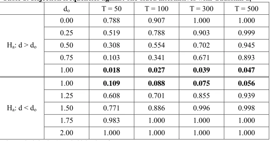
do =1 will indicate the size of the test. We see in this table that the sizes of the tests are

clearly biased if the sample size is small. Thus, for example, if T = 50 and the tests are

directed against d > do, the size is 0.018; however, when directed against d < do, it

becomes much higher than the nominal size of 0.050 (0.109); however, as the sample

size increases the values tend to approximate to the 5% level, which is consistent with

the asymptotic nature of the tests. If we focus now on the rejection frequencies, we

observe that the higher sizes observed in the case of d < do also produce higher rejection

probabilities in all cases compared with the case of alternatives with d < 1.

Nevertheless, for departures higher than 0.5 even with small sample sizes, the tests

behave fairly well, and if T ≥ 300 the probabilities are very close to 1 in all cases.

Remember here that the null consists of a unit root with Chebyshev polynomials, so the

test performs well even in strong nonstationary contexts. Performing the experiment

with -coefficients different from 1, and also with other values of d lead to essentially

the same conclusions implying that the test performs relatively well if the sample sizeis

large enough.

Table 1: Rejection frequencies against one-sided alternatives with Gaussian ut

do T = 50 T = 100 T = 300 T = 500

Ha: d > do

0.00 0.788 0.907 1.000 1.000

0.25 0.519 0.788 0.903 0.999

0.50 0.308 0.554 0.702 0.945

0.75 0.103 0.341 0.671 0.893

1.00 0.018 0.027 0.039 0.047

Ha: d < do

1.00 0.109 0.088 0.075 0.056

1.25 0.608 0.701 0.855 0.939

1.50 0.771 0.886 0.996 0.998

1.75 0.983 1.000 1.000 1.000

2.00 1.000 1.000 1.000 1.000

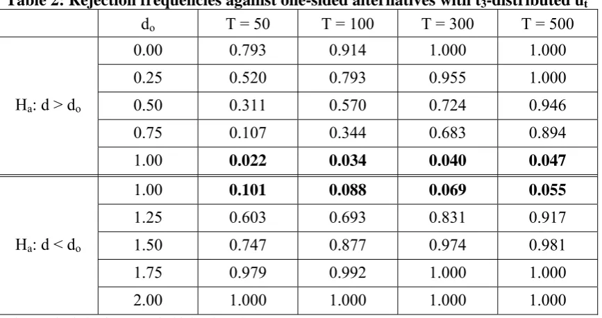
Table 2: Rejection frequencies against one-sided alternatives with t3-distributed ut

do T = 50 T = 100 T = 300 T = 500

Ha: d > do

0.00 0.793 0.914 1.000 1.000

0.25 0.520 0.793 0.955 1.000

0.50 0.311 0.570 0.724 0.946

0.75 0.107 0.344 0.683 0.894

1.00 0.022 0.034 0.040 0.047

Ha: d < do

1.00 0.101 0.088 0.069 0.055

1.25 0.603 0.693 0.831 0.917

1.50 0.747 0.877 0.974 0.981

1.75 0.979 0.992 1.000 1.000

2.00 1.000 1.000 1.000 1.000

The nominal size is 5%. In bold the size of tests.

Next we perform a similar experiment in non-Gaussian contexts. For this

purpose, we examine the same null model as in Table 1 but assuming now that the

disturbances are t-Student distributed with 3 degrees of freedom. This distribution is

interesting because it just satisfies the second moment condition required in the test, its

third moments not existing. The results, displayed in Table 2, are competitive with the

Gaussian ones, with the sizes being closer to the nominal one of 5% in practically all

cases. If we focus on the rejection frequencies, they tend to be slightly larger for values

of do < 1, and lower when do > 1 compared with Table 1. Very similar results were

obtained if weak autocorrelation is permitted for the I(0) disturbances term, and the

same applies for other values of d in (14).

5. An empirical application

In this section we apply the fractional integration tests developed in this paper to

examine the mean reversion of real exchange rates and purchasing power parity (PPP).

countries should converge when measured in the same currency, so as to equalize the

purchasing power of the currencies. This, therefore, implies that the real exchange rate,

defined as the ratio of prices in both places, translated to a common currency using the

nominal exchange rate, should converge to 1. However, it is well known within the

literature that the absolute version of the PPP hypothesis may be too restrictive. Hence,

a less restrictive version of PPP is the relative PPP hypothesis, which implies that prices

in common currency may converge to a constant different from 1. This relative version

of PPP implies then that what is actually expected in the long run is that the real

exchange rate should be reverting to a constant, which may be different from 1. The

intuition behind this is related to the fact that because of the existence of trade barriers,

transport costs, and different measures of price indices, there may be a gap between

price levels in different countries. Hence, on average, changes in real exchange rates

should be zero, according to the relative version of the PPP theory.

In view of the above comments, testing for mean reversion becomes of

paramount importance when testing for the empirical validity of the PPP theory, which

at the same time, can be seen as a measure of the degree of over/under-valuation of the

currencies, and it is used as a base for a number of macroeconomic models, e.g. the

Dornbusch model. However, real exchange rate convergence, on average, to a constant

along time may not be very realistic, in particular when countries experience different

levels of economic growth and productivity gains, as well as, when countries suffer

from changes in economic fundamentals, which may indeed change the equilibrium

value of real exchange rates. For instance, the well known dynamic Penn effect and the

Balassa-Samuelson effect, may induce deterministic trends in the data (see Lothian and

Taylor, 2000, among others), and the existence of structural changes, may, in addition,

deterministic trends when testing for real exchange rate mean reversion. In a recent

contribution, Cushman (2008) tests for the PPP hypothesis using the Bierens (1997) unit

root tests for bilateral exchange rates. He finds evidence to support that real exchange

rates may in fact contain non-linear trends. However, it is not possible to test for the

significance of these trends, unless the null is rejected.

Our newly developed fractional integration testing procedure, taking into

account Chebyshev polynomials to approximate non-linear deterministic trends, solves

these problems with the flexibility of having non-integer orders of integration. Given

that the residuals of the auxiliary regression are I(0) stationary by assumption, t

-statistics are valid to test for the significance of the non-linear trends. This novelty

solves the problem of choosing the order of the Chebyshev polynomials, which was not

clearly defined by Bierens (1997).

The data used in the empirical application are real effective exchange rates

against each country’s 27 main trade partners, downloaded from Eurostat (code

ert_eff_ic_q) for 40 countries, with different degrees of economic integration and

development. We have used quarterly data from 1994:Q1 until 2011:Q3.

Across this section we consider the following model,





 

  m

i

t t d t

iT i

t P t x L x u

y

0

, )

1 ( , )

(

   (17)

assuming that ut is a white noise process.

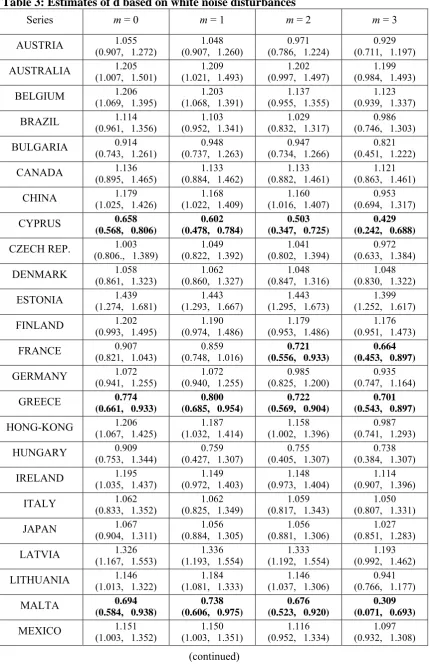
Table 3 displays the estimates of d and the 95% confidence bands of the

non-rejection values of d for the cases of m = 0, 1, 2 and 3. Higher values of m lead to

non-significant coefficients for i in all cases. These estimates were obtained using the

Whittle function in the frequency domain and they coincide with the values of do that

produce the lowest statistics in absolute value when using our testing approach with a

Table 3: Estimates of d based on white noise disturbances

Series m = 0 m = 1 m = 2 m = 3

AUSTRIA 1.055

(0.907, 1.272)

1.048 (0.907, 1.260)

0.971 (0.786, 1.224)

0.929 (0.711, 1.197)

AUSTRALIA 1.205

(1.007, 1.501)

1.209 (1.021, 1.493)

1.202 (0.997, 1.497)

1.199 (0.984, 1.493)

BELGIUM 1.206

(1.069, 1.395)

1.203 (1.068, 1.391)

1.137 (0.955, 1.355)

1.123 (0.939, 1.337)

BRAZIL 1.114

(0.961, 1.356)

1.103 (0.952, 1.341)

1.029 (0.832, 1.317)

0.986 (0.746, 1.303)

BULGARIA 0.914

(0.743, 1.261)

0.948 (0.737, 1.263)

0.947 (0.734, 1.266)

0.821 (0.451, 1.222)

CANADA 1.136

(0.895, 1.465)

1.133 (0.884, 1.462)

1.133 (0.882, 1.461)

1.121 (0.863, 1.461)

CHINA 1.179

(1.025, 1.426)

1.168 (1.022, 1.409)

1.160 (1.016, 1.407)

0.953 (0.694, 1.317)

CYPRUS 0.658

(0.568, 0.806)

0.602 (0.478, 0.784)

0.503 (0.347, 0.725)

0.429 (0.242, 0.688)

CZECH REP. 1.003

(0.806., 1.389)

1.049 (0.822, 1.392)

1.041 (0.802, 1.394)

0.972 (0.633, 1.384)

DENMARK 1.058

(0.861, 1.323)

1.062 (0.860, 1.327)

1.048 (0.847, 1.316)

1.048 (0.830, 1.322)

ESTONIA 1.439

(1.274, 1.681)

1.443 (1.293, 1.667)

1.443 (1.295, 1.673)

1.399 (1.252, 1.617)

FINLAND 1.202

(0.993, 1.495)

1.190 (0.974, 1.486)

1.179 (0.953, 1.486)

1.176 (0.951, 1.473)

FRANCE 0.907

(0.821, 1.043)

0.859 (0.748, 1.016)

0.721 (0.556, 0.933)

0.664 (0.453, 0.897)

GERMANY 1.072

(0.941, 1.255)

1.072 (0.940, 1.255)

0.985 (0.825, 1.200)

0.935 (0.747, 1.164)

GREECE 0.774

(0.661, 0.933)

0.800 (0.685, 0.954)

0.722 (0.569, 0.904)

0.701 (0.543, 0.897)

HONG-KONG 1.206

(1.067, 1.425)

1.187 (1.032, 1.414)

1.158 (1.002, 1.396)

0.987 (0.741, 1.293)

HUNGARY 0.909

(0.753, 1.344)

0.759 (0.427, 1.307)

0.755 (0.405, 1.307)

0.738 (0.384, 1.307)

IRELAND 1.195

(1.035, 1.437)

1.149 (0.972, 1.403)

1.148 (0.973, 1.404)

1.114 (0.907, 1.396)

ITALY 1.062

(0.833, 1.352)

1.062 (0.825, 1.349)

1.059 (0.817, 1.343)

1.050 (0.807, 1.331)

JAPAN 1.067

(0.904, 1.311)

1.056 (0.884, 1.305)

1.056 (0.881, 1.306)

1.027 (0.851, 1.283)

LATVIA 1.326

(1.167, 1.553)

1.336 (1.193, 1.554)

1.333 (1.192, 1.554)

1.193 (0.992, 1.462)

LITHUANIA 1.146

(1.013, 1.322)

1.184 (1.081, 1.333)

1.146 (1.037, 1.306)

0.941 (0.766, 1.177)

MALTA 0.694

(0.584, 0.938)

0.738 (0.606, 0.975)

0.676 (0.523, 0.920)

0.309 (0.071, 0.693)

MEXICO 1.151

(1.003, 1.352)

1.150 (1.003, 1.351)

1.116 (0.952, 1.334)

1.097 (0.932, 1.308)

NETHERLANDS 1.088

(0.932, 1.304)

1.082 (0.924, 1.301)

1.081 (0.922, 1.303)

1.034 (0.861, 1.262)

NORWAY 0.944

(0.729, 1.222)

0.952 (0.741, 1.222)

0.949 (0.731, 1.229)

0.943 (0.722, 1.221)

NEW ZEELAND 1.274

(1.039, 1.624)

1.265 (1.044, 1.603)

1.264 (1.034, 1.603)

1.255 (1.033, 1.566)

POLAND 1.029

(0.804, 1.354)

1.034 (0.823, 1.346)

1.023 (0.796, 1.346)

0.997 (0.741, 1.331)

PORTUGAL 1.051

(0.872, 1.292)

1.039 (0.855, 1.288)

1.039 (0.853, 1.288)

0.984 (0.762, 1.244)

ROMANIA 1.145

(0.931, 1.433)

1.134 (0.917, 1.433)

1.133 (0.917, 1.435)

1.129 (0.906, 1.422)

RUSSIAN FED. 1.245

(1.022, 1.533)

1.249 (1.042, 1.553)

1.242 (1.027, 1.556)

1.242 (1.027, 1.554)

SOUTH KOREA 1.094

(0.861, 1.411)

1.096 (0.873, 1.417)

1.096 (0.876, 1.417)

1.083 (0.846, 1.407)

SLOVAKIA 1.137

(0.984, 1.417)

1.107 (0.944, 1.395)

0.992 (0.722, 1.366)

0.980 (0.692, 1.354)

SLOVENIA 1.342

(1.037, 1.755)

1.337 (1.072, 1.744)

1.342 (1.077, 1.711)

1.332 (1.054, 1.591)

SPAIN 0.907

(0.813, 1.047)

0.859 (0.744, 1.016)

0.721 (0.554, 0.933)

0.664 (0.459, 0.899)

SWEDEN 1.063

(0.854, 1.376)

1.044 (0.807, 1.377)

1.044 (0.803, 1.364)

1.042 (0.797, 1.382)

SWITZERLAND 1.252

(1.096, 1.463)

1.207 (1.076, 1.398)

1.208 (1.073, 1.384)

1.207 (1.066, 1.373)

TURKEY 0.824

(0.643, 1.308)

0.677 (0.318, 1.269)

0.678 (0.317, 1.263)

0.648 (0.207, 1.255)

U.K. 1.227

(1.082, 1.433)

1.228 (1.087, 1.444)

1.151 (0.956, 1.405)

1.132 (0.933, 1.388)

U.S.A 1.212

(1.047, 1.346)

1.213 (1.045, 1.467)

1.172 (0.983, 1.444)

1.119 (0.911, 1.393) Note: In bold, evidence of mean reversion (d < 1). In brackets we display the confidence intervals at the 95%.

of d are very similar across the different values for m, in general, observing a slight

reduction in the degree of integration as weincrease m.4 We also notice that most of the

estimates of d are within the unit root interval and some of them are even significantly

above 1. The only evidence of mean reversion (i.e. d significantly below 1) is obtained

for the cases of Cyprus, Greece and Malta (for all values of m) and for France and Spain

4

 This might indicate a degree of competition between the non-linear structure due to the Chebyshev polynomials and the I(d) framework in describing the structure of the series. 

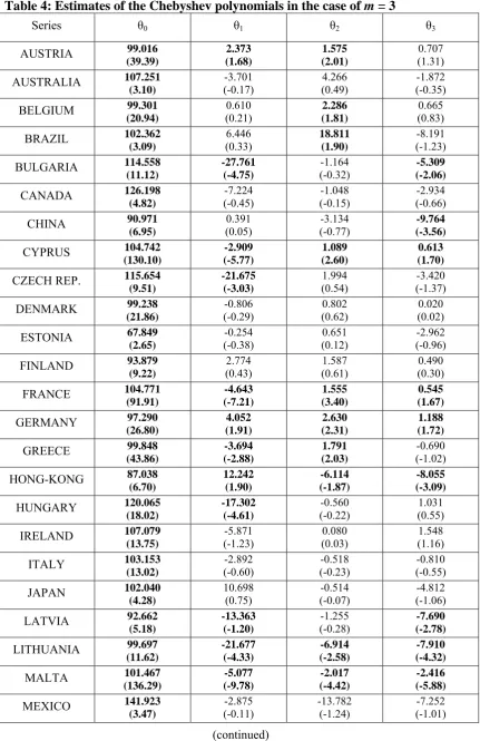
Table 4: Estimates of the Chebyshev polynomials in the case of m = 3

Series 0 1 2 3

AUSTRIA 99.016

(39.39) 2.373 (1.68) 1.575 (2.01) 0.707 (1.31)

AUSTRALIA 107.251

(3.10) -3.701 (-0.17) 4.266 (0.49) -1.872 (-0.35)

BELGIUM 99.301

(20.94) 0.610 (0.21) 2.286 (1.81) 0.665 (0.83)

BRAZIL 102.362

(3.09) 6.446 (0.33) 18.811 (1.90) -8.191 (-1.23)

BULGARIA 114.558

(11.12) -27.761 (-4.75) -1.164 (-0.32) -5.309 (-2.06)

CANADA 126.198

(4.82) -7.224 (-0.45) -1.048 (-0.15) -2.934 (-0.66)

CHINA 90.971

(6.95) 0.391 (0.05) -3.134 (-0.77) -9.764 (-3.56)

CYPRUS 104.742

(130.10) -2.909 (-5.77) 1.089 (2.60) 0.613 (1.70)

CZECH REP. 115.654

(9.51) -21.675 (-3.03) 1.994 (0.54) -3.420 (-1.37)

DENMARK 99.238

(21.86) -0.806 (-0.29) 0.802 (0.62) 0.020 (0.02)

ESTONIA 67.849

(2.65) -0.254 (-0.38) 0.651 (0.12) -2.962 (-0.96)

FINLAND 93.879

(9.22) 2.774 (0.43) 1.587 (0.61) 0.490 (0.30)

FRANCE 104.771

(91.91) -4.643 (-7.21) 1.555 (3.40) 0.545 (1.67)

GERMANY 97.290

(26.80) 4.052 (1.91) 2.630 (2.31) 1.188 (1.72)

GREECE 99.848

(43.86) -3.694 (-2.88) 1.791 (2.03) -0.690 (-1.02)

HONG-KONG 87.038

(6.70) 12.242 (1.90) -6.114 (-1.87) -8.055 (-3.09)

HUNGARY 120.065

(18.02) -17.302 (-4.61) -0.560 (-0.22) 1.031 (0.55)

IRELAND 107.079

(13.75) -5.871 (-1.23) 0.080 (0.03) 1.548 (1.16)

ITALY 103.153

(13.02) -2.892 (-0.60) -0.518 (-0.23) -0.810 (-0.55)

JAPAN 102.040

(4.28) 10.698 (0.75) -0.514 (-0.07) -4.812 (-1.06)

LATVIA 92.662

(5.18) -13.363 (-1.20) -1.255 (-0.28) -7.690 (-2.78)

LITHUANIA 99.697

(11.62) -21.677 (-4.33) -6.914 (-2.58) -7.910 (-4.32)

MALTA 101.467

(136.29) -5.077 (-9.78) -2.017 (-4.42) -2.416 (-5.88)

MEXICO 141.923

NETHERLANDS 102.410 (21.65) -1.291 (-0.45) 0.254 (0.18) 1.339 (1.50)

NORWAY 104.085

(11.81) -1.934 (-0.37) 0.741 (0.27) -0.730 (-0.39)

NEW ZEELAND 87.099

(2.01) 7.085 (0.26) 2.264 (0.22) 3.277 (0.52)

POLAND 108.376

(5.03) -11.451 (-0.90) -3.565 (-0.55) -3.853 (-0.90)

PORTUGAL 101.431

(34.79) -3.058 (-1.78) -0.064 (-0.07) 0.906 (1.54)

ROMANIA 119.977

(3.29) -22.595 (-1.01) -1.933 (-0.20) -1.976 (-0.32)

RUSSIAN FED. 99.158

(0.93) -13.008 (-0.19) 12.455 (0.49) -1.812 (-0.11)

SOUTH KOREA 110.881

(3.08) 6.752 (0.31) -1.080 (-0.10) 3.805 (0.57)

SLOVAKIA 131.870

(10.30) -34.771 (-4.61) 7.797 (2.02) -1.482 (-0.57)

SLOVENIA 86.649

(5.25) -0.551 (-0.05) 0.370 (0.09) -0.693 (-0.32)

SPAIN 104.771

(91.91) -4.643 (-7.21) 1.554 (3.40) 0.545 (1.73)

SWEDEN 95.991

(8.10) 4.633 (0.65) 0.266 (0.07) -0.599 (-0.27)

SWITZERLAND 93.915

(4.87) 8.133 (0.67) 0.222 (0.04) -0.632 (-0.21)

TURKEY 111.308

(11.74) -16.485 (-3.07) 0.170 (0.04) -1.649 (-0.54)

U.K. 97.291

(5.72) 2.831 (0.27) -8.440 (-1.88) -2.380 (-0.84)

U.S.A 112.153

(4.76) 1.777 (0.12) -8.525 (-1.35) -5.725 (-1.43) In bold, significant coefficients at the 5% level. T-statistics are given in brackets.

if m = 2 or 3, i.e. assuming the existence of non-linearities. The results from Table 3

also point out that it is possible to reduce the order of integration of the variable by

increasing artificially the order of the Chebyshev polynomials, m. This is consistent

with other works that show that fractional integration and nonlinearities are issues

which are intimately related (Diebold and Inoue, 2001; Granger and Hyung, 2004).

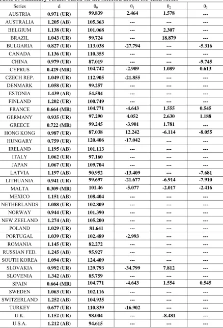
Next we examine the deterministic terms in more detail, checking whether the

Chebyshev coefficients are statistically significant for the selected estimates of d. The

present. Based on these significant terms, we selected the appropriate model for each

series, and the summary of the results (based only on the significant Chebyshev

coefficients) are reported in Table 5. We see that strong evidence of non-linearities

(with the two non-linear coefficients statistically significantly different from zero) is

obtained for the cases of Cyprus, France, Malta, Spain, Germany, Hong-Kong and

Lithuania. In the first four cases, the unit root hypothesis is rejected in favour of mean

reversion, while in the remaining three cases, though the estimated values of d are

smaller than 1, the unit root cannot be rejected. Evidence of non-linearity with

significant 2-coefficient is observed for Austria, Greece and Slovakia, the unit root

being rejected in favor of mean reversion in the case of Greece. Also, for some

countries only one of the two non-linear coefficients is significant, such as China (with

only 3 being statistically significant, and an estimate of d of 0.979) as well as Bulgaria

and Latvia (with d equal to 0.827 and 1.197 respectively), and also, Belgium, Brazil and

the UK (with 2 significant but not 3) and the unit root being not rejected. For the

remaining cases, only an intercept or a linear trend is required.

We also conducted the analysis based on weakly autocorrelated errors. We tried

both seasonal and non-seasonal autoregressions and the results, not displayed, indicate

that though quantitatively there are some differences when computing the results based

on autocorrelated errors qualitatively the same conclusions hold, since the number of

cases corresponding to “mean reversion”, “unit roots” or “explosive roots” affect

exactly to the same series as in the case of white noise errors.

Our results pinpoint a few economic insights. We first observe that in most cases

structural breaks in the form of non-linear trends are present in the data. Second, for a

number of countries, for instance the Czech Republic and Hungary, a linear trend is

Table 5: Summary results based on the selected model for each series

Series d 0 1 2 3

AUSTRIA 0.971 (UR) 99.839 2.464 1.578 ---

AUSTRALIA 1.205 (AB) 105.363 --- --- ---

BELGIUM 1.138 (UR) 101.068 --- 2.307 ---

BRAZIL 1.043 (UR) 99.724 --- 18.879 ---

BULGARIA 0.827 (UR) 113.038 -27.794 --- -5.316

CANADA 1.136 (UR) 110.355 --- --- ---

CHINA 0.979 (UR) 87.019 --- --- -9.745

CYPRUS 0.429 (MR) 104.742 -2.909 1.089 0.613

CZECH REP. 1.049 (UR) 112.905 -21.855 --- ---

DENMARK 1.058 (UR) 99.257 --- --- ---

ESTONIA 1.439 (AB) 54.584 --- --- ---

FINLAND 1.202 (UR) 100.749 --- --- ---

FRANCE 0.664 (MR) 104.771 -4.643 1.555 0.545

GERMANY 0.935 (UR) 97.290 4.052 2.630 1.188

GREECE 0.722 (MR) 99.245 -3.901 1.781 ---

HONG KONG 0.987 (UR) 87.038 12.242 -6.114 -8.055

HUNGARY 0.759 (UR) 120.406 -17.042 --- ---

IRELAND 1.195 (AB) 101.113 --- --- ---

ITALY 1.062 (UR) 97.160 --- --- ---

JAPAN 1.067 (UR) 109.704 --- --- ---

LATVIA 1.197 (AB) 90.952 -13.409 --- -7.681

LITHUANIA 0.941 (UR) 99.697 -21.677 -6.914 -7.910

MALTA 0.309 (MR) 101.46 -5.077 -2.017 -2.416

MEXICO 1.151 (AB) 108.404 --- --- ---

NETHERLANDS 1.088 (UR) 102.809 --- --- ---

NORWAY 0.944 (UR) 101.390 --- --- ---

NEW ZEELAND 1.274 (AB) 105.200 --- --- ---

POLAND 1.029 (UR) 81.641 --- --- ---

PORTUGAL 1.039 (UR) 102.489 -2.993 --- ---

ROMANIA 1.145 (UR) 82.272 --- --- ---

RUSSIAN FED. 1.245 (AB) 95.927 --- --- ---

SOUTH KOREA 1.094 (UR) 124.409 --- --- ---

SLOVAKIA 0.992 (UR) 129.793 -34.799 7.812 ---

SLOVENIA 1.342 (AB) 85.759 --- --- ---

SPAIN 0.664 (MR) 104.771 -4.643 1.554 0.545

SWEDEN 1.063 (UR) 102.116 --- --- ---

SWITZERLAND 1.252 (AB) 104.935 --- --- ---

TURKEY 0.677 (UR) 110.839 -16.902 --- ---

U.K. 1.152 (UR) 98.004 --- -8.481 ---

U.S.A. 1.212 (AB) 94.615 --- --- ---

be present, which makes economic sense given the process of catching-up with Western

Europe during the transition period from communism to market economies. Finally, that

in all cases of mean reversion, it occurs along with structural breaks. Comparing our

results to those by Cushman (2008), although the results are not directly comparable, we

can say that we find evidence of mean reversion using a lower order for the Chebyshev

polynomials.

5. Concluding comments

In this paper we have examined a model that incorporates Chebyshev polynomials in

time in the context of long range dependence. For the latter we use a very general

expression that permits us to examine stationary and nonstationary hypotheses with one

or more unit root or fractional degrees of integration with the singularities in the

spectrum occurring at zero and non-zero frequencies. The main advantage of this model

is that combining the two structures (non-linear Chebyshev polynomials and fractional

integration) leads to a new model that is linear in parameters, permitting the estimation

of the Chebyshev polynomials in a very simple way. Moreover, we describe a testing

procedure, originally proposed by Robinson (1994) that displays several advantages in

the present context. Thus, it allows us to test any real vector value for the differencing

parameters, including stationary and nonstationary hypotheses; the incorporation of the

Chebyshev polynomials allows its estimation with a straightforward method, including

the use of the significancy of the coefficients throughout standard t-values. The limit

distribution of the procedure is standard chi-squared distributed, and several Monte

samples. A small empirical application based on this approach and using real effective

References

Andel, J. (1986) Long memory time series models, Kybernetika 22, 105-123.

Bierens, H.J. (1997) Testing the unit root with drift hypothesis against nonlinear trend

stationarity with an application to the US price level and interest rate, Journal of

Econometrics 81, 29-64.

Bloomfield, P. (1973) An exponential model in the spectrum of a scalar time series,

Biometrika 60, 217-226.

Chung, C.-F. (1996a) A generalized fractionally integrated autoregressive

moving-average process, Journal of Time Series Analysis17, 111-140.

Chung, C.-F. (1996b) Estimating a generalized long memory process, Journal of

Econometrics 73, 237-259.

Cushman, D. O. (2008) Real exchange rates may have nonlinear trends, International

Journal of Finance and Economics 13, 158-173.

Dalla, V. and J. Hidalgo (2005) A parametric bootstrap test for cycles, Journal of

Econometrics 129, 219-261.

Diebold, F.X. and A. Inoue (2001) Long memory and regime switching. Journal of

Econometrics 105, 131-159.

Diebold, F. X. and G. D. Rudebusch (1989) Long memory and persistence in aggregate

output, Journal of Monetary Economics 24, 189-209.

Ferrara, L. and D. Guegan (2001), Forecasting with k-factor Gegenbauer processes:

Theory and Applications, Journal of Forecasting 20, 581-601.

Gil-Alana, L. A. (2001) Testing stochastic cycles in macroeconomic time series, Journal

Gil-Alana, L. A. (2004) The use of Bloomfield (1973) model as an approximation to

ARMA processes in the context of fractional integration, Mathematical and Computer

Modelling 39, 429-436.

Gil-Alana, L. A. and P. M. Robinson (1997) Testing of unit roots and other

nonstationary hypotheses in macroeconomic time series, Journal of Econometrics 80,

241-268.

Gil-Alana, L.A. and P.M. Robinson (2001) Testing of seasonal fractional integration in

the UK and Japanese consumption and income, Journal of Applied Econometrics 16,

95-114.

Giraitis, L. and P. Leipus (1995) A generalized fractionally differencing approach in

long memory modelling, Lithuanian Mathematical Journal 35, 65-81.

Granger, C. W. J. (1980) Long memory relationships and aggregation of dynamic

models, Journal of Econometrics 14, 227-238.

Granger, C.W.J. and N. Hyung (2004) Occasional structural breaks and long memory

with an application to the S&P 500 absolute stock returns, Journal of Empirical Finance

11, 399-421.

Granger, C. W. J. and R. Joyeux (1980) An introduction to long memory time series and

fractional differencing, Journal of Econometrics 16, 121-130.

Gray, H. L., N. F. Zhang and W. A. Woodward (1989) On generalized fractional

processes, Journal of Time Series Analysis 10, 233-257.

Gray, H.L., N. F. Zhang and W. A. Woodward (1994) On generalized fractional

processes. A correction, Journal of Time Series Analysis 15, 561-562.

Hamming, R. W. (1973) Numerical Methods for Scientists and Engineers, Dover.

Lee, J. and M. C. Strazicich (2003) Minimum LM unit root test with two structural

breaks, Review of Economics and Statistics 85, 1082-1089.

Lothian, J. And M. P. Taylor (2000) Purchasing power parity over two centuries:

strengthening the case for real exchange rate stability. A reply to Cuddington and Liang,

Journal of International Money and Finance 19, 759-764.

Lumsdaine, L. and D. Papell (1997) Multiple trend breaks and the unit-root hypothesis,

Review of Economics and Statistics 79, 212-218.

Magnus, W., F. Oberhettinger and R. P. Soni (1966) Formulas and theorems for the

special functions of mathematical physics, Springer, Berlin.

Ouliaris, S., J. Y. Park and P. C. B. Phillips (1989) Testing for a unit root in the

presence of a maintained trend. In Ray, B. (Ed.) Advances in Econometrics and

Modelling. Kluwer, Dordrecht, 6-28.

Papell, D. and R. Prodan (2006) Additional evidence of long-run purchasing power

parity with restricted structural change, Journal of Money, Credit and Banking 38,

1329-1349.

Perron, P. (1989) The great crash, the oil price shock and the unit root hypothesis,

Econometrica 57, 1361-1402.

Porter-Hudak, S. (1990) An application of the seasonal fractionally differenced model

to the monetary aggregate, Journal of the American Statistical Association 85, 338-344.

Press, W. H., B. P. Flannery, S. A. Teukolsky and W. T. Wetterling (1986) Numerical

recipes. The art of scientific computing, Cambridge University Press, Cambridge.

Rainville, E.D. (1960) Special functions, MacMillan, New York.

Ray, B.K. (1993) Long range forecasting of IBM product revenues using a seasonal

Robinson, P.M. (1994) Efficient tests of nonstationary hypotheses, Journal of the

American Statistical Association 89, 1420-1437.

Sadek, N. and A. Khotanzad (2004) K-factor Gegenbauer ARMA process for network

traffic simulation, Computers and Communications 2, 963-968.

Sowell, F. (1992) Modelling long run behavior with the fractional ARIMA model,

Journal of Monetary Economics 29, 277-302.

Sutcliffe, A. (1994) Time series forecasting using fractional differencing, Journal of

Forecasting 13, 383-393.

Woodward, W. A., Q. C. Cheng and H. L. Ray (1998) A k-factor Gamma long memory

model, Journal of Time Series Analysis 19, 485-504.

Zivot, E. and D. W. K. Andrews (1992) Further evidence on the great crash, the oil

price shock, and the unit root hypothesis, Journal of Business and Economic Statistics