Robust PID based indirect-type iterative learning control for batch processes with time-varying uncertainties

This is a repository copy of Robust PID based indirect-type iterative learning control for batch processes with time-varying uncertainties.

White Rose Research Online URL for this paper: http://eprints.whiterose.ac.uk/109321/

Version: Accepted Version

Article:

Liu, T, Wang, XZ and Chen, J (2014) Robust PID based indirect-type iterative learning control for batch processes with time-varying uncertainties. Journal of Process Control, 24 (12). pp. 95-106. ISSN 1873-2771

https://doi.org/10.1016/j.jprocont.2014.07.002

© 2014. This manuscript version is made available under the CC-BY-NC-ND 4.0 license http://creativecommons.org/licenses/by-nc-nd/4.0/ ↗

[email protected] https://eprints.whiterose.ac.uk/

Reuse

Unless indicated otherwise, fulltext items are protected by copyright with all rights reserved. The copyright exception in section 29 of the Copyright, Designs and Patents Act 1988 allows the making of a single copy solely for the purpose of non-commercial research or private study within the limits of fair dealing. The publisher or other rights-holder may allow further reproduction and re-use of this version - refer to the White Rose Research Online record for this item. Where records identify the publisher as the copyright holder, users can verify any specific terms of use on the publisher’s website.

Takedown

If you consider content in White Rose Research Online to be in breach of UK law, please notify us by

Robust PID based indirect-type iterative learning control for batch

processes with time-varying uncertainties

Tao Liu

_{, Xue Z. Wang}

_{, Junghui Chen}

a Institute of Advanced Control Technology, Dalian University of Technology, Dalian, 116024, P. R. China

b Institute of Particle Science and Engineering, School of Process, Environmental and Materials

Engineering, University of Leeds, Leeds LS2 9JT, UK

c Department of Chemical Engineering, Chung-Yuan Christian University, Chung-Li, 320, Taiwan

* Corresponding author. Tel: + 86-411-84706465; Fax: + 86-411-84706706 E-mail addresses: [email protected] (T. Liu), [email protected] (X. Wang),

[email protected] (J. Chen)

Abstract: Based on the proportional- integral-derivative (PID) control structure widely used in engineering applications, a robust indirect-type iterative learning control (ILC) method is proposed for industrial batch processes subject to time- varying uncertainties. An important merit is that the proposed ILC design is independent of the PID tuning that aims primarily to hold robust stability of the closed-loop system, owing to the fact that the ILC updating law is implemented through adjusting the setpoint of the closed-loop PID control structure plus a feedforward control to the plant input from batch to batch. According to the robust H infinity control objective, a robust discrete-time PID tuning algorithm is given in terms of the plant state-space model description to accommodate for time-varying process uncertainties. For the batchwise direction, a robust ILC updating law is developed based on the two-dimensional (2D) control system theory. Only measured o utput errors of current and previous cycles are used to implement the proposed ILC scheme for the convenience of practical application. An illustrative example from the literature is adopted to demonstrate the effectiveness and merits of the proposed ILC method.

1

Introduction

Iterative learning control (ILC) method can be adopted to realize perfect tracking or control optimization for industrial and chemical batch processes, owing to the use of repetitive operation information from historical cycles. With the wide application of ILC in engineering applications in the recent years, it has become increasingly appealing to develop robust ILC methods to deal with time- varying uncertainties occurring in a cycle or cycle-to-cycle (batchwise) uncertainties, because many batch processes, e.g., industrial injection molding and pharmaceutical crystallization, are slowly varying from batch to batch, while repeating fundamental dynamic response characteristics [1-4]. As surveyed by Bonvin et al [5], Ahn et al [6], and Wang et al [7], most of existing references have been devoted to time- invariant linear or nonlinear batch processes. The developed robust ILC methods have been in general classified into two types [7], one is called direct-type that means the ILC design integrates the feedback control (responsible for closed- loop stability and no steady output deviation) and the feedforward control (responsible for the setpoint tracking) through the identical closed- loop controller, and another is called indirect-type which implies that either the feedback or the feedforward control could be implemented through different controllers that may be designed relatively independent.

For the indirect-type ILC, the control structure is typically composed of two loops, one loop constructed in terms of a conventional controller like PID, and another loop used for adjusting the setpoint or the process input similar to a feedforward control manner. Based on the internal model control (IMC) structure, a learning setpoint design was proposed [22] to robustly track the setpoint profile against the process input delay uncertainty. By comparison, a P-type learning algorithm was presented to adjust the setpoint in combination with the model prediction control (MPC) method for tracking the desired profile, which was successfully used to the control of artificial pancreatic beta-cell [23]. Based on the conventional PID control structure, a parallel learning-type PID was added to improve the setpoint tracking performance without sacrificing the closed- loop stability [24]. An alternative anticipatory-type ILC (A-ILC) was developed to adjust the setpoint in terms of the PID control loop for robust tracking of the desired profile [25]. The robust stability condition of a learning-type setpoint design in terms of a PI control loop was analyzed in the recent paper [26]. A quadratic criterion was presented to analyze the ILC convergence in terms of a MPC structure for time-varying linear systems [27]. The achievable tracking performance of an indirect-type ILC scheme was assessed by estimating the minimum output variance bound [28]. Combining with the feedback control design, a two-step ILC design [29] was proposed to adjust the process input for improving the output tracking performance against load disturbance and process uncertainties. For highly nonlinear processes such as crystallization processes, hierarchical ILC and nonlinear MPC based ILC methods [30, 31] were proposed to track the desired setpoint profile against batch-to-batch uncertainties.

indirect-type ILC scheme. Accordingly, the PID tuning and the ILC design can be made relatively independent of each other in the proposed control scheme, and more flexibility is introduced to devise the control system robust stability and tracking performance, respectively. By establishing the sufficient conditions in terms of linear matrix inequality (LMI) constraints for maintaining robust stability of the PID control loop and the robust convergence of the ILC scheme, respectively, the PID and ILC controllers are derived along with an adjustable robust H infinity performance level. The effectiveness of the proposed method is demonstrated through a n illustrative example from the literature. For clarity, the paper is organized as follows: Section 2 briefly describes a batch process with time- varying uncertainties by using a state-space model with norm-bounded uncertainties, and then introduces the proposed indirect-type ILC scheme based on the conventional PID control structure. Correspondingly, a robust PID tuning method is proposed in terms of the robust H infinity control objective in Section 3. By formulating the learning setpoint strategy and feedforward control in the frame of a 2D system, section 4 presents the proposed ILC design by establishing the sufficient LMI conditions to hold the 2D system asymptotic stability. Section 5 shows an illustrative example to demonstrate the effectiveness and merits of the proposed ILC method. Conclusions are drawn in Section 6.

Throughout this paper, the following notations are used: n m denotes a n m real matrix space. For any matrix Pm m , P0 (or P 0) means P is a positive (or semipositive) definite symmetric matrix, in which the symmetric elements are indicated by ‘*’. T

P denotes the transpose of P. diag{ } denotes a block-diagonal matrix. For any vector x and matrix

0

P  , denote V x_P( ) x 2_P x PxT . The identity or zero vector (or matrix) with appropriate dimension is denoted by I or 0 . For a 2D signal, z i j( , ) , if

2

2 0 0

( , ) n m ( , )

i j

z i j 

 

2

Problem formulation

: P_

m m

p

( 1, 1) [ ( , 1)] ( , 1) [ ( , 1)] ( , 1) ( , 1) ( , 1) ( , 1), 0 ;

(0, 1) (0), =0,1, .

x t k A A t k x t k B B t k u t k t k

y t k Cx t k t T

x k x k



              



    



 _{ }



(1)

where t and k denotes the time and batch indices, respectively, and k1 indicates the current batch (or cycle). _{x t k}( ,  1) nx _{denote the state variables, u t k( ,}  ₁₎ nu _{the control} inputs, ( , 1) ny

y t k  the process outputs. Denote by A and _m B the nominal state matrices, _m and by A t k( , 1) and B t k( , 1) time- varying uncertainties that are not repetitive from cycle to cycle and practically specified as A t k( ,    1) A_{1 1}( )t A₂, B t k( ,    1) B_{1 2}( )t B₂, where A₁, A₂, B₁, and B₂ are constant matrices, and Ti ( )t i( )t I , i1, 2. Denote

by Tp the time period of each cycle, and x(0) is the initial resetting condition of each cycle.

Note that other process uncertainties such as from input actuator and output measurement may also be lumped into A t k( , 1) and B t k( , 1) for analysis.

The control objective is to determine a control law such that the system output can track the desired output profile (or target output trajectory) as close as possible against the process uncertainties and/or load disturbance.

To design an indirect-type ILC scheme, we define the output error in the current cycle (k1) by

r

( , 1) Y ( ) ( , 1)

e t k t y t k (2 )

where Y ( )_r t denotes the desired output profile, and y t k( , 1) the real output in the current cycle. Correspondingly, the time integral of e t k( , 1) is denoted by e t k( , 1), i.e.

0

( , 1) ( , 1)

t

i

e t k e i k



  



By comparison, we define the setpoint tracking error in the current cycle by

s( , 1) y ( ,s 1) ( , 1)

e t k t k y t k (4)

where y t k_s( , 1) denotes the setpoint command in the current cycle, which is different with the desired output profile,Y ( )_r t , in that it is adjusted real-time in an indirect-type ILC scheme for tracking Y ( )r t .

s( , 1) s( 1, 1) s( , 1)

e t k e t k e t k

        , 0 t T_p (5)

Moreover, we define a batchwise error function by

( , 1) ( , 1) ( , ) f t k f t k f t k

    (6)

where f may denote x , y , s u , e , e , or s , respectively.

It follows from (1) using the definitions in (2) and (6) that

( , 1) ( , ) ( , 1)

e t k e t k C x t k  (7)

x t( 1,k 1) [A_m A t k( , 1)]x t k( ,  1) [B_m B t k( , 1)]u t k( ,  1) ( ,t k1) (8) where

( ,t k 1) [ A t k( , 1) A t k x t k( , )] ( , ) [ B t k( , 1) B t k u t k( , )] ( , ) ( ,t k 1)

              (9)

It is obvious that ( ,t k 1) 0 for any non-repeatable parameter uncertainties and varied initial process conditions from batch to batch, and therefore can be viewed as a non-repeatable load disturbance to deal with.

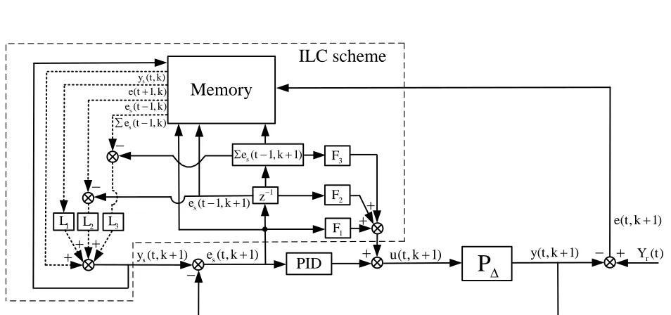
Based on the conventional PID control structure, the proposed indirect-type ILC scheme is shown in Figure 1, as outlined by the dash- line box, where the learning controllers, L , 1 L , 2 L , 3

are set to adjust the setpoint command, i.e.

s( , 1) s( , ) 1 ( 1, ) 2 s( 1, 1) 3 s( 1, 1)

y t k y t k L e t k L e t  k Le t k (10)

where y t k denotes the setpoint input in the previous cycle, and _s( , ) e t( 1, )k the one-step ahead output error in the previous cycle. It follows from (4), (5), and (6) that

s( 1, 1) s( 1, 1) s( 1, )

e t k e t k e t k

        (11)

s( , 1) s( 1, 1) s( , 1)

e t k e t k e t k

        (12)

It is seen from (10)-(12) that the tracking errors of e t( 1, )k , e t_s( 1, )k , e t k , and _s( , )

s( 1, )

e t k

  in the previous cycle are used to construct the ILC updating law added to the

setpoint command in the current cycle, relatively independent of the closed- loop PID control structure shown in Figure 1.

In Figure 1, the feedforward controllers, F , 1 F , 2 F , are used to adjust the process input, 3

PID 1 s 2 s 3 s

( , 1) ( , 1) ( , 1) ( 1, 1) ( 1, 1)

u t k u t k F e t k F e t k F e t k (13)

where u_PID is the PID control output. The setpoint tracking errors at the current moment and one-step ahead moment, and the error integral in the current cycle are used to construct the feedforward control in the proposed scheme.

Hence, the proposed ILC scheme (outlined by the dash- line box in Figure 1) and the closed-loop PID control can be designed separately, as detailed in the following two sections.

3

Robust PID tuning

According to the process state-space description in (1), by omitting the batch index for brevity due to its irrelevance to the PID tuning in the proposed control scheme shown in Figure 1, a PID control law is generally expressed in the following form,

PID( ) p ( ) i ( ) d[ ( 1) ( )]

u t k e t  k e t k e t e t (14)

where k_p, k , and _i k are the proportional, integral, and derivative parameters of PID, _d respectively. Note that because e t( 1) cannot be measured at the current moment for implementing u t( ) , the differential signal of e t(  1) e t( ) is practically substituted by

( ) ( 1)

e t e t , [ ( )e t e t(  2) 2 (e t1)] / 2, or adding a low-pass filter for execution but at the expense of somewhat performance degradation [32].

By introducing an auxiliary state variable, e t( ), we establish the augmented control system description,





( 1) ( )

( ( ) ( )

( ) ( 1)

( ) ( )

( 1)

x t A x t B

u t t

e t C e t

x t y t C

e t



         

  

_  _ _{ }     

       

  



 

 _

 

 _{  }



0

0 0

0

I I

(15)

where AA_m A t( ) and BB_m B t( ).

Substituting (2) with Y ( )_r t 0 (which has no influence to the closed- loop stability) into (14) in terms of the nominal process model described by (1) (i.e. A t( )0 and B t( )0) yields,

1 1 1

PID( ) ( d m) ( p i) ( ) ( d m) i ( 1) ( d m) d( m) ( )

Let

1

p d m p i

ˆ _{( ) ( )}

k  Ik CB  k k (17)

1

i d m i

ˆ _{( )}

k  Ik CB  k (18)

1

d d m d

ˆ _{( )}

k  Ik CB  k (19) Then, substituting (14) and (17)-(19) into (15) yields the closed-loop system,





d m p i

ˆ ˆ ˆ

( 1) _{[ ( ) ]} ( )

( )

( ) ( 1)

( ) ( )

( 1)

x t _{A B k C A k C Bk} x t

t

e t _C e t

x t

y t C

e t     _       _ _{ }  _{    }               _    _{  }  0 0 I I I (20)

For tuning the PID controller to maintain the control system robust stability, the H infinity control objective is adopted here, i.e.

PID

2 2

( ) ( )

e t 





where _PID denotes the robust performance level.

To achieve the H infinity control objective, we give the following theorem,

Theorem 1: The PID cont rol system in (20) subject to time-varying process uncertainties shown

in (1) is guaranteed robustly stable with a H infinity control performance level, PID, if there

exist P₁₁0, P₂₂0, matrices P , ₁₂ R , ₁ R , and positive scala rs ₂ ₁, ₂, such that the following LMI holds,

1 A1 A1 2 B1 B1 g

A2 B2 PID PID 1 2 * * * 0 * * * * * * * * * * * * T T

T T T T

P D

P PH C P P

                _{  }     _         _        

0 0 0

0

0 0 0

0 0 0 I I I I (22)

where D_g [I 0]T, H [I 0],   _A1 [ A₁T, ]0T,   _A2 [ A P_{2 11}, A P_{2 12}],   _B1 [ B₁T, ]0T,

B2 [ B R2 1, B R2 2]

11 12

22 *

P P

P

P

 

  

 ,

m 11 m 1 m 12 m 2

11 12 12 22

T

A P B R A P B R

CP P CP P

 

 

   _{   } 

 

by parameterizing

1

d m p i 1 2

ˆ ˆ ˆ

[k C( IA )k C k] [ R R P]  (23)

Proof: See the Appendix I.

It can be seen from (17)-(19) and (23) that the PID parameters may be retrieved by prescribing the derivative parameter(s), k , that is, when _d k is specified, the other parameters d

can be obtained using (19) as

i ˆi( d m)

k k Ik CB (24)

p ˆp( d m) i

k k Ik CB k (25)

Note that letting k_d 0 leads to a PI controller, which is preferred for practical application owing to the implemental simplicity.

To achieve good robust control performance, the PI (by letting kd 0) or PID controller can

be determined by performing the following optimization program,

PID ( ), ( )

Minimize

A t B t 

  (26) In fact, a smaller value of _PID leads to a more aggressive control action and vice versa. Therefore, a trade-off should be made between the achievable control performance and the control action generated by the designed PI or PID controller. In consideration of that the closed- loop controller is primarily used for maintaining the control system robust stability, it is preferred to take a PI controller for implementation if such a controller can be derived from the above optimization program, compared to a PID controller which requires a practical implementation of the ideal derivative action that may degrade the closed- loop robust stability or control performance.

4

Robust indirect-type ILC design

synthetically analyzing the 2D stability against process uncertainties and load disturbance. A preliminary knowledge of a 2D system stability is presented as below.

Consider a 2D Roesser’s system [33],





11 11 12 12

21 21 22 22

1 2

( 1, ) ( , )

( , )

( , 1) ( , )

( , ) ( , )

( , )

, =0,1,2, .

h h

v v

h

v

A A A A

x i j x i j

i j

A A A A

x i j x i j

x i j y i j C C

x i j

i j               _   _{   }           _{ }  _          (27)

where _xhn1 _{is the horizontal state vector, x}vn2 _{the vertical state vector, y the system} output,  load disturbance, A₁₁ , A₁₂ , A₂₁ , and A₂₂ denote the state matrices uncertainties. The boundary condition of the Roesser’s system is denoted by

ˆ( ) [ h(0, )] , [T v( , 0)]T T x t   x j x i _ .

Lemma 1 [ 26] : If there exist positive definite matrices, P1 0 and P2 0, such that the

following LMI holds

A PA PT  0 (28)

where

11 11 12 12

21 21 22 22

A A A A

A

A A A A

   

 

  _{   } 

 , Pdiag P P{ , }1 2

then the 2D Roesser’s system in (27) with 0 is asymptotically stable. In addition, if (0, ) 0

h

x j  , there exists a positive scalar (0,1) such that

0 0

2 2

0 0

[ ( , 1)] [ ( , )]

I I

v v

P P

i i

V x i j  V x i j

 

 





x i

 . (29)

According to the proposed ILC scheme shown in Figure 1, it follows from (4), (6), and (7) that

s( , 1) s( , ) s( , 1) ( , 1)

y t k y t k e t k C x t k  (30)

Substituting (30) into (10) yields

s( , 1) 1 ( 1, ) 2 s( 1, 1) 3 s( 1, 1) ( , 1)

e t k L e t k L e t k L e t k C x t k

Then, substituting (31) into (12) obtains

s( , 1) 1 ( 1, ) 2 s( 1, 1) ( 3) s( 1, 1) ( , 1)

e t k L e t k L e t k L e t k C x t k

         I       (32)

Substituting the PID control law of (14) with e t(  1) e t( ) replaced by e t( )e t( 1) into (13), we obtain

p s i s d s s

1 s 2 s 3 s

p i d 1 s 2 d s i 3 s

( , 1) ( , 1) ( , 1) [ ( , 1) ( 1, 1)]

( , 1) ( 1, 1) ( 1, 1)

( ) ( , 1) ( ) ( 1, 1) ( ) ( 1, 1)

u t k k e t k k e t k k e t k e t k

F e t k F e t k F e t k

k k k F e t k F k e t k k F e t k

          

        

             

( 33)

Note that the ideal derivative term in (14) is substituted by a practical form of e t( )e t( 1)

for obtaining (33). Other practical forms may also be adopted to derive u t k( , 1) and are omitted herein.

Correspondingly, it follows that

p i d 1 s 2 d s i 3 s

( , 1) ( ) ( , 1) ( ) ( 1, 1) ( ) ( 1, 1)

u t k k k k F e t k F k e t k k F e t k

                  (34)

Based on the robust PID design given in Section 2, by substituting (31), (32), and (34) into (8), we obtain

p i d 1

p i d 1 1

p i d 1 2 2 d s

p i d 1

( 1 , 1 ) [ ( ) ] ( , 1 )

( ) ( 1, )

[( ) ] ( 1, 1) [(

x t k A B k k k F C x t k

B k k k F L e t k

B k k k F L F k e t k

B k k k F

 



       

    

       

    ) _{3 3 i}] _s( 1, 1)

( , 1)

L F k e t k

t k          (35)

where AA_m A t k( , 1) and BBm B t k( , 1).

Consequently, the predicted output error can be derived in terms of (7) as

p i d 1

p i d 1 1

p i d 1 2 2 d s

( 1 , 1 ) ( 1 , ) ( 1 , 1 )

[ ( ) ] ( , 1 [ ( ) ] ( 1 , [ ( ) ]

e t k e t k C x t k

C A C B k k k F C x t k

C B k k k F L e t k

C B k k k F L F k e t k

                              I

p i d 1 3 3 i s

1) [( ) ] ( 1, 1) ( , 1)

CB k k k F L F k e t k

C t k

              (36)

s s

w

s s

s

s

( 1, 1) ( , 1)

( , 1) ( 1, 1)

( )

( , 1) ( 1, 1)

( 1, 1) ( 1, )

( , 1) ( 1, 1) ( , 1)

( 1, 1) ( 1, )

x t k x t k

e t k e t k

D t

e t k e t k

e t k e t k

x t k

e t k

t k G

e t k

e t k

                   _   _{ }    _{ } _           _{ }   _              _{ }               _{  }  (37)

where G[0 0 0 I , ] D_w [I 0 0 CT T] ,

p i d 1 p i d 1 2 2 d

2

2

p i d 1 p i d 1 2 2 d

p i d 1 3 3 i p i d 1 1

3 1

3 1

p i d 1 3 3 i

( ) [( ) ]

( ) [( ) ]

[( ) ] ( )

[( ) ]

A B k k k F C B k k k F L F k

C L

C L

CA CB k k k F C CB k k k F L F k

B k k k F L F k B k k k F L

L L

L L

CB k k k F L F k

           _     _                             I

I CB k( _p k_i k_d F L₁) ₁

         _

Note that ( ,t k 1) e t( 1, )k can be regarded as the controlled variable to be minimized against process uncertainties, possibly varied initial process conditions from batch to batch, and load disturbance. That is to say, the robust 2D control objective can be determined in terms of a batch process control specification [21] as

1 p 2

2 2

1

BP ILC 2 ILC 2

0 0

( ( , 1) ( , 1) ) 0

N T N

t k

J   t k   t k

    



 

By defining

s

s

( , 1)

( , ) ( 1, 1)

( 1, 1)

h

x t k

x t k e t k

e t k

        _   _       

, x t kv( , )e t( 1, )k (39)

the 2D system in (37) can be viewed as a typical Roesser’s system in the form of (27).

Theorem 2: The 2D control system in (37) subject to time-varying process uncertainties

described by (1) is gua ranteed robustly stable with a H infinity control performance level, _ILC, if there exist Q₁ 0, Q₂ 0, Q₃ 0, Q₄ 0, matrices F , ˆ₂ F , ˆ₃ L , ˆ₁ L , ˆ₂ L , and positive ˆ₃ scalars ₁, ₂, such that the following LMI holds,

1 A1 A1 2 B1 B1 w

A2 B2 ILC ILC 1 2 * * * 0 * * * * * * * * * * * * T T

T T T

Q D

Q QG P P

                _{  }     _         _        

0 0 0

0

0 0 0

0 0 0 I I I I (40)

where Qdiag Q Q{ , _{1 2}, Q₃, Q₄},D_g [I 0]T , H[I 0],   _A1 [ A₁T, , , 0 0  A C₁T T T] ,

A2 [ A2, , , ]

   0 0 0 , _B1 [ ₁T, , , ₁T T T]

B B C

   0 0   ,

B2 2 p i d 1 2 p i d 1 2 2 d

2 p i d 1 3 3 i 2 p i d 1 1

ˆ ˆ

( ) , [( ) ],

ˆ ˆ ˆ

[( ) ], ( )

B k k k F C B k k k F L F k

B k k k F L F k B k k k F L



  _         



          _

m 1 m p i d 1 1 m p i d 1 2 m 2 m d 2

1 2

1 2

m 1 m p i d 1 1 m p i d 1 2 m 2 m d 2

m p i d 1 3 m 3 m i 3 m p i d 1 1

3 ˆ ˆ ( ) ( ) ˆ ˆ ˆ ˆ ( ) ( )

ˆ ˆ ˆ

( ) ( )

ˆ ˆ

A Q B k k k F CQ B k k k F L B F B k Q

CQ L

CQ L

CA Q CB k k k F CQ CB k k k F L CB F CB k Q

B k k k F L B F B k Q B k k k F L

L                                       1

3 3 1

m p i d 1 3 m 3 m i 3 4 m p i d 1 1

ˆ ˆ

ˆ ˆ ˆ

( ) ( )

L

Q L L

CB k k k F L CB F CB k Q Q CB k k k F L

     _            _ (41) by parameterizing 1 1 1 4

1 2 2 2

1 3 3 3

ˆ ˆ ˆ L L Q

L L Q

L L Q

      _     (42) 1

2 2 2

1 3 3 3

ˆ ˆ

F F Q

F F Q       

 (43)

Note that the feedforward controller, F , is prescribed for solving the LMI condition in (40). ₁ To facilitate the feasibility of the LMI condition in (40), the choice of F should be made to ₁ keep all the eigenvalues of A_m B k_m( _p  k_i k_d F C₁) in the unit circle in the z-transfer plane, i.e.

m m p i d 1

eig[ ( ) ] 1

i A B k k k F C

       , i1, 2, ,nx. (44)

In fact, all the feedforward controllers, F , ₁ F , ₂ F , corresponding to ₃ F , ₁ F , ˆ₂ F in (40) ˆ₃ that may be viewed as slack variables to facilitate the LMI feasibility, are used to increase the flexibility of the indirect-type ILC in the proposed control scheme shown in Figure 1, for the purpose of robustly tracking the desired output profile against process uncertainties and load disturbance.

To obtain the optimal robust tracking performance, the ILC controllers can be determined by performing the following optimization program,

ILC ( ), ( )

Minimize

A t B t 

  (45) Similarly, by specifying the learning controllers, L , ₁ L , ₂ L , which determine the ₃ convergence rate of the ILC scheme, the achievable robust performance can be assessed through the LMI condition in (40), and so is for the allowable process uncertainty bounds denoted by

( , 1) A t k

  and B t k( , 1). Note that the allowable variation of initial process conditions from

batch to batch can also be assessed through the LMI condition in (40) by lumping the variation bound into the magnitude (D ) of the disturbance as shown in (9) and (37). _w

5

Illustration

cycle to cycle. Based on open- loop tests and analysis, a model of the nozzle pressure response to the hydraulic valve input signal was identified [10] as

1 ( ) : P z_ 

1 2

1 2

1.239( 5%) 0.9282( 5%)

( , 1) ( , 1) ( , 1)

1 1.607( 5%) 0.6086( 5%)

z z

y t k u t k t k

z z 

 

 

  

    

   

where the percentages in parentheses indicate the parameter perturbations in the worst case of cyclic operation.

For application of the proposed method, we write the above model in the following state-space form,

: P_

 

1.607 1 1.239 1

( 1, 1) ( ) ( , 1) ( ) ( , 1) ( , 1)

0.6086 0 0.9282 0

( , 1) 1, 0 ( , 1)

x t k A x t k B u t k t k

y t k x t k

  _{  }  _{   }  _{   }  _  _  _            _{  } 

0.0804 ( ) 0 1 0 ( ) 0 0.0804 0 ( )

0.0304 ( ) 0 0 1 0 ( ) 0.0304 0

t t A t t t              _{  } _{    }          

0.062 ( ) 1 0 ( ) 0 0.062

( )

0.0464 ( ) 0 1 0 ( ) 0.0464

t t B t t t              _{  } _{    }          

where ( )t is a time-varying factor along either the time or batchwise direction and ( )t 1. By performing the optimization procedure in (26), we obtain the minimal H infinity robust performance level, PID* 1.28. To avoid over aggressive control signal, we take PID5 to

solve the LMI condition in (22), obtaining the PI controller parameters, kp 1.2889 and

i 0.0336

k  . For the ILC design, it can be easily verified that the range of F₁ [ 1.3, 0.1] can ensure all the eigenvalues of A_m B k_m( _p  k_i k_d F C₁) located in the unit circle in the z-transfer plane. We choose F₁  0.5 to perform the optimization procedure in (40), obtaining the minimal H infinity robust performance level, ILC* 110, and correspondingly, L10.1776,

2 0

L  , L3  0.029, F2 0, and F3  0.0097.

The target profile (Y ) takes the following form as adopted in the cited references [10, 26], r

r

p

200, 0 100;

200+5( 100), 100 120;

300, 120 200.

t

Y t t

t T     _     _{  } 

Case 1. Time- invariant process uncertainties. In this case, A t( ) and B t( ) are assumed to be fixed as their upper bounds. The tracking results are shown in Figure 2 (a) and (b), while the output tracking error in terms of the following criterion is plotted in Figure 3,

p

p 1

ATE( ) ( , ) / T

t

k e t k T







It is seen that perfect tracking is reached through 20 cycles by the proposed method after an initial run of the PID tuning, compared to the cited paper [26] which needed almost 50 cycles to realize perfect tracking. Moreover, there exists no steady output tracking error in each cycle, owing to using the output tracking error in the current cycle for 2D ILC design as shown in (37).

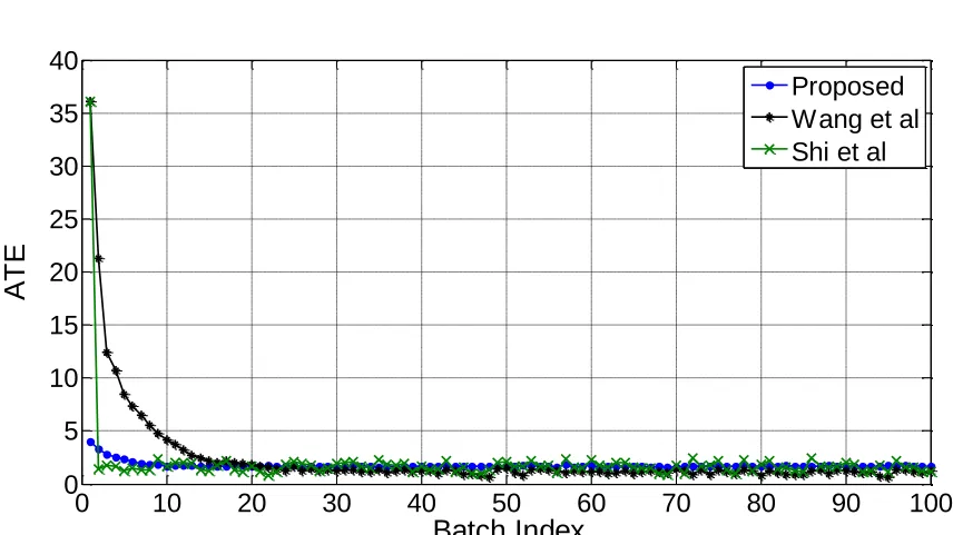
Case 2. Time-varying uncertainties and disturbance. Assume that the process state transfer

matrices becomes time-varying with ( )t 0.1, together with non-repetitive load disturbance,

( ,t k 1) sin(t ( ))k

    where ( )k is a random variable uniformly distributed in the range of

[0, 2 ] as assumed in the cited paper [26]. Since the closed-loop system becomes a stochastic process, we perform 100 Monte Carlo tests, each of which includes 100 cycles. The averaged results of ATE are plotted in Figure 4, in comparison with those of refs. [10, 26]. It is seen that the closed-loop system maintains robust stability well in both the time and batchwise directions by the proposed ILC method, thus demonstrating that it can be reliably used for robust tracking of the desired profile and on- line optimization against batch-to-batch process uncertainties and load disturbance.

6

Conclusions

from the LMI conditions established for maintaining the closed-loop robust stability. For the batchwise direction, an ILC scheme consisting of a learning setpoint strategy and a feedforward control added to the process input has been developed based on an equivalent 2D system description of the batch process and the LMI condition formulated in terms of the robust H infinity control objective for robust convergence. Only measured output errors of current and previous cycles are used to implement the proposed ILC scheme for the convenience of practical application. The application to an illustrative example from the literature has demonstrated the effectiveness and merits of the proposed ILC method.

Acknowledgement

This work is supported in part by the National Thousand Talents Program of China, the Fundamental Research Funds for the Central Universities of China, and the National Science Council, R.O.C.

Appendix I

Proof of Theorem 1

Define the following Lyapunov-Krasovskii inequality of state energy to guarantee the asymptotic stability of the closed-loop system shown in (20),

2 2

1

PID 2 PID 2

ˆ ˆ

[ ( 1)] [ ( )] ( ( ) ( ) )

P P

V x t V x t    e t   t (A1) where x tˆ( )[x tT( ), e t( 1) ]T T, and PID is the robust performance level as shown in (21).

Considering that e t( ) Cx t( ) by letting Y ( )r t 0, and x t( )[ , ] ( )I 0 x tˆ , we have

ˆ

( ) ( )

e t  CHx t (A2) where H has been shown in (22).

By substituting (20) into (A1), we obtain

1 0

T

   (A3)

where  [x tˆT( ), T( )]t T, D_g [I 0]T, and

d m p i

g

ˆ ˆ ˆ

[ ( ) ]

A B k C A k C Bk

A

C

    

  



 

I

1

g PID

1 g g

g * PID

T T T

T

A P H C CH

P A D

D      _{ }       _{ }        0

I (A5)

By the Schur complement, it can be derived that (A3) is guaranteed by

g PID PID * 0 * * * * * T T P D

P PH C

      _   _{ }  _         0 0 0 I I (A6) where

11 d m p 11 12 12 d m p 12 22

11 12 12 22

ˆ ˆ ˆ ˆ ˆ ˆ

[ ( ) ] i T [ ( ) ] i

T

AP B k C A k C P Bk P AP B k C A k C P Bk P

CP P CP P

 _{       }            I I (A7)

Note that  can be reformulated as

A1 1( )t A2 B1 2( )t B2

           (A8)

where  , _A1 , _A2 , _B1 , and _B2 have been shown in (22),

1 [ (ˆd m) ˆp ] 11 ˆ 12 T i

R  k CIA k C P k P and R₂ [ (k Cˆ_d IA_m)k C Pˆ_p ] ₁₂k Pˆ_{i 22}.

The following lemma is used herein for analysis.

Lemma 2 [ 34] : Let A, D, E, and F be real matrices of appropriate dimensions with 1

F  , the following inequality holds for any scalar  0,

1

T T T T T

DFEE F D DD  E E (A9)

Using Lemma 2 and the Schur complement, it can be seen that (A6) is guaranteed by (22) in Theorem 1. This completes the proof.

Appendix II

Proof of Theorem 2

The robust 2D control objective in (38) can be rewritten as

1 p 2 1 p 2

2 2

1

BP ILC 2 ILC 2

0 0 0 0

( ( , 1) ( , 1) ) 0

N T N N T N

t k t k

J   t k   t k V V

   



   



 

 

( 1, ) ( , )

( , 1) ( , )

h h

Q _v Q _v

x t k x t k

V V V

x t k x t k

    

  _{ } _{ }



    (A11)

Using the boundary conditions from an initial resetting of batch process operation, i.e.

s s s

s s s

(0, 0) (0,1) (1, 0) 0; (0, 0) (0,1) (1, 0) 0;

(0, 0) (0,1) (1, 0) 0; (0, 0) (0,1) (1, 0) 0.

x x x

e e e

e e e

e e e

              _{  }           _{  }  (A12)

it can be easily verified using Qdiag Q Q{ , _{1 2}, Q₃, Q₄} that



1 p 2 1 p 2

1 1 2

2 3 3

s

0 0 0 0

s s s

[ ( 1, 1)] [ ( , 1)] [ ( , 1)]

[ ( 1, 1)] [ ( , 1)] [ ( 1, 1)]

N T N N T N

Q Q Q

t k t k

Q Q Q

V V x t k V x t k V e t k

V e t k V e t k V e t k

                               

 

 

V_Q[ (e t1,k1)]V_Q [ (e t1, )]k

2 2

1 2

2 1

3 4

1 s 1

0 0

s 1 2

0 0

[ ( 1, 1)] [ ( , 1)]

[ ( , 1)] [ ( 1, 1)]

0 N N Q Q k k N N Q Q k t

V x N k V e N k

V e N k V e t N

                     









Therefore, a sufficient condition to ensure the control objective in (A10) is that

2 2

1

ILC ( ,t k 1) 2 ILC ( ,t k 1)2 V 0

  _{ }  _{   }

(A14)

By substituting the 2D system description in (37) and (A11) into (A14), we obtain

2 0

T

   (A15)

where   [x t kh( , )] , [T x t kv( , )] , T T( )t _T, and

1 ILC 2 w ILC w * T T T

Q G G

Q D D      _{ }     _{  } __{ }     0

I (A16)

By the Schur complement, it can be derived that (A15) is guaranteed by

A1 1( )t A2 B1 2( )t B2

           (A18)

where , _A1, _A2, _B1, and _B2 have been shown in (40).

References

[1] D.E. Seborg, T.F. Edgar, D.A. Mellichamp, Process Dynamic and Control, 2nd Edition, John Wiley & Sons, New Jersey, 2004.

[2] F. Gao, Y. Yang, C. Shao, Robust iterative learning control with applications to injection molding process, Chemical Engineering Science 56 (2001) 7025-7034.

[3] Z.K. Nagy, J.W. Chew, M. Fujiwara, R.D. Braatz, Comparative performance of concentration and temperature controlled batch crystallizations, Journal of Process Control 18 (2008) 399-407.

[4] Z.K. Nagy, Model based robust control approach for batch crystallization product design, Computers & Chemical Engineering 33(10) (2009) 1685-1691.

[5] D. Bonvin, B. Srinivasan, D. Hunkeler, Control and optimization of batch processes, IEEE Trans. Control Systems Magazine 26(6) (2006) 34-45.

[6] H.-S. Ahn, Y.Q. Chen, K. L. Moore, Iterative learning control: Brief survey and categorization, IEEE Trans. Systems, Man, and Cybernetics-Part C: Applications and Reviews, 37(6) (2007) 1099-1121.

[7] Y. Wang, F. Gao, F. Doyle, Survey on iterative learning control, repetitive control, and run-to-run control, Journal of Process Control 19(10) (2009) 1589-1600.

[8] Z. Xiong, J. Zhang, Product quality trajectory tracking in batch processes using iterative learning control based on time- varying perturbation models, Ind. Eng. Chem. Res. 42 (2003) 6802-6814.

[9] A. Tayebi, C.J. Chien, A unified adaptive iterative learning control framework for uncertain nonlinear systems, IEEE Tran. Autom. Control 52 (2007) 1907-1913.

[10] J. Shi, F. Gao, T.-J. Wu, Integrated design and structure analysis of robust iterative learning control system based on a two-dimensional model, Ind. Eng. Chem. Res. 44 (2005) 8095-8105.

[12] C. Mi, H. Lin, Y. Zhang, Iterative learning control of antilock braking of electric and hybrid vehicles, IEEE Tran. Vehicular Technology 54 (2005) 486-494.

[13] C.H. Li, P.L. Tso, Experimental study on a hybrid-driven servo press using iterative learning control, International Journal of Machine Tools and Manufacture 48 (2008) 209-219.

[14] D.I. K im, S. K im, An iterative learning control method with application for CNC machine tools, IEEE Tran. Industry Applications 32 (1996) 66-72.

[15] X. Ruan, Z. Bien, K.H. Park, Decentralized iterative learning control to large-scale industrial processes for nonrepetitive trajectory tracking, IEEE Tran. Systems, Man, and Cybernetics - Part A: Systems and Humans 38 (2008) 238-252.

[16] A. Tayebi, Analysis of two particular iterative learning control schemes in frequency and time domains, Automatica 43 (2007) 1565-1572.

[17] J. Shi, F. Gao, T.-J. Wu, From two-dimensional linear quadratic optimal control to iterative learning control. Paper 1. Two-dimensional linear quadratic optimal controls and system analysis, Ind. Eng. Chem. Res. 45 (2006) 4603-4616.

[18] J. Shi, F. Gao, T.-J. Wu, From two-dimensional linear quadratic optimal control to iterative learning control. Paper 2. Iterative learning controls for batch processes, Ind. Eng. Chem. Res. 45 (2006) 4617-4628.

[19] J. Shi, F. Gao, T.-J. Wu, Robust iterative learning control design for batch processes with uncertain perturbations and initialization, AIChE Journal 52(6) (2006) 2171-2187.

[20] T. Liu, F. Gao, Robust two-dimensional iterative learning control for batch processes with state delay and time-varying uncertainties, Chemical Engineering Science 65(23) (2010) 6134-6144.

[21] T. Liu, Y. Wang, A synthetic approach for robust constrained iterative learning control of piecewise affine batch processes, Automatica 48(11) (2012) 2762-2775.

[22] T. Liu, F. Gao, Y. Wang, IMC-based iterative learning control for batch processes with uncertain time delay, Journal of Process Control 20(2) (2010) 173-180.

(2010) 173-180.

[24] K. Tan, S. Zhao, J.X. Xu, O nline automatic tuning of a proportional integral derivative controller based on an iterative learning control approach, IET Control Theor. Appl. 1(1) (2007) 90-96.

[25] J. Wu, H. Ding, Reference adjustment for a high-acceleration and high-precision platform via A-type of iterative learning control, Proc. IMechE, Part I: J. Syst. Control Eng. 221 (2007) 781–789.

[26] Y. Wang, T. Liu, Z. Zhao, Advanced PI control with simple learning set-point design: Application on batch processes and robust stability analysis, Chemical Engineering Science 71(1) (2012) 153-165.

[27] J.H. Lee, K.S. Lee, W.C. K im, Model-based iterative learning control with a quadratic criterion for time-varying linear systems, Automatica 36 (2000) 641-657.

[28] J. Chen, C.-K. Kong, Performance assessment for iterative learning control of batch units, Journal of Process Control 19 (2009) 1043-1053.

[29] I. Chin, S.J. Q in, K.S. Lee, M. Cho, A two-stage iterative learning control technique combined with real-time feedback for independent disturbance rejection, Automatica 40 (2004) 1913-1922.

[30] N. Sanzida, Z.K. Nagy, Iterative learning control for the systematic design of supersaturation controlled batch cooling crystallisation processes, Computers & Chemical Engineering 59 (2013) 111-121.

[31] M. W. Hermanto, R.D. Braatz, M.-S. Chiu, Integrated batch-to-batch and nonlinear model predictive control for polymorphic transformation in pharmaceutical crystallization, AIChE Journal 57(4) (2011) 1008-1019.

[32] K.J. Åström, T. Hägglund, PID Controller: Theory, Design, and Tuning, 2nd Edition, ISA Society of America, Research Triangle Park, NC, 1995.

[33] T. Kaczorek, Two-dimensional linear system, Berlin: Springer-Verlag, 1985.

List of Figure Captions

Figure 1 Block diagram of the proposed PID based indirect-type ILC scheme Figure 2 Tracking performance for case 1

Figure 3 Plot of ATE for case 1 Figure 4 Plot of ATE for case 2

Figure 1 Block diagram of the proposed PID based indirect-type ILC scheme

Memory

( , 1)

u t k y t k( , 1)

s( , 1)

e t k

P

( , 1) e t k

  

s( 1, 1)

e t k

  

1

z

PID

s( , 1)

y t k

s( 1, 1)

e t k

1

F

3

F

2

F

 

3

L

s( , )

y t k

s( 1, )

e t k

s( 1, )

e t k

 

( 1, )

e t k



 

1

L L2

 



(a)

(b)

Figure 2 Tracking performance for case 1

0 20 40 60 80 100 120 140 160 180 200 -50

0 50 100 150 200

Step (t)

In

p

u

t

si

g

n

a

l

Batch 1 Batch 2 Batch 20 0 20 40 60 80 100 120 140 160 180 200 0

50 100 150 200 250 300 350

Step (t)

P

ro

ce

ss o

u

tp

u

t

Desired profile Batch 1

Batch 2 Batch 20

0 10 20 30 40 160

Figure 3 Plot of ATE for case 1

Figure 4 Plot of ATE for case 2

1 2 3 4 5 6 7 8 9 10 11 12 13 14 15 16 17 18 19 20 0

5 10 15 20 25 30 35 40 45 50

Cycle Number

A

T

E

Proposed Wang et al

0 10 20 30 40 50 60 70 80 90 100 0

5 10 15 20 25 30 35 40

Batch Index

A

T

E