White Rose Research Online URL for this paper:
http://eprints.whiterose.ac.uk/81905/
Version: Accepted Version
Article:
Lin, Z and Kwan, RSK (2014) A two-phase approach for real-world train unit scheduling.
Public Transport, 6 (1-2). 35 - 65. ISSN 1866-749X
https://doi.org/10.1007/s12469-013-0073-9
[email protected] https://eprints.whiterose.ac.uk/
Reuse
Unless indicated otherwise, fulltext items are protected by copyright with all rights reserved. The copyright exception in section 29 of the Copyright, Designs and Patents Act 1988 allows the making of a single copy solely for the purpose of non-commercial research or private study within the limits of fair dealing. The publisher or other rights-holder may allow further reproduction and re-use of this version - refer to the White Rose Research Online record for this item. Where records identify the publisher as the copyright holder, users can verify any specific terms of use on the publisher’s website.
Takedown
If you consider content in White Rose Research Online to be in breach of UK law, please notify us by
Noname manuscript No. (will be inserted by the editor)
A Two-phase Approach for Real-world Train Unit
Scheduling
Zhiyuan Lin · Raymond S. K. Kwan
Abstract A two-phase approach for the train unit scheduling problem is proposed. The first phase assigns and sequences train trips to train units temporarily ignor-ing some station infrastructure details. Real-world scenarios such as compatibility among traction types and banned/restricted locations and time allowances for cou-pling/decoupling are considered. Its solutions would be near-operable. The second phase focuses on satisfying the remaining station detail requirements, such that the solutions would be fully operable.
The first phase is modeled as an integer fixed-charge multicommodity flow (FCMF) problem. A branch-and-price approach is proposed to solve it. Experiments have shown that it is only capable of handling problem instances within about 500 train trips. The train company collaborating in this research operates over 2400 train trips on a typical weekday. Hence, a heuristics has been designed for compacting the prob-lem instance to a much smaller size before the branch-and-price solver is applied. The process is iterative with evolving compaction based on the results from the previous iteration thereby converging to near-optimal results.
The second phase is modeled as a multidimensional matching problem with a mixed integer linear programming (MILP) formulation. A column-and-dependent-row generation method for it is under development.
Keywords train unit scheduling·railway shunting·fixed-charge multicommodity flow·branch-and-price·hybridization method
JEL Code C60·C61·R40
Z. Lin
School of Computing, University of Leeds, Leeds, LS2 9JT, United Kingdom Tel.: +44 (0)113 343 5430, Fax: +44 (0)113 343 5468, E-mail: [email protected]
R. S. K. Kwan
1 Introduction
A train multiple unit, ortrain unit, is a set of train carriages with its own built-in engine(s). Without a locomotive, it is able to move in both directions on its own. A train unit can also be coupled with other units of the same or similar types.Train unit schedulingrefers to the planning of how timetabled train trips (or simplytrains) in one operational day are sequenced to be operated by each train unit in the com-pany’s fleet. Usually performed after the timetable has been fixed, and followed by a subsequent crew scheduling stage, train unit scheduling is also calledtrain unit
di-agrammingin the UK, where aunit diagramis a documentation of the sequence of
trains and other auxiliary activities, e.g. coupling/decoupling and shunting, an indi-vidual train unit will serve on a specified day of operation.
Optimization in train unit scheduling is very important because of the high costs associated with leasing, operating and maintaining a fleet. It would also impact upon the subsequent planning of crew resources. For some heavily used commuter net-works, e.g. in the North and South of England, train unit scheduling is also impor-tant for best distributing limited rolling stock resources, by coupling/decoupling train units and/or running them empty, to meet passenger demands. In real-world practice, there are often thousands of timetabled trains to be scheduled and complex rail in-frastructure layouts, especially at large train stations, making train unit scheduling optimization a very hard problem to solve.
In this paper, a two-phase approach is proposed. The first phase is mainly atrain
sequencing and fleet assignment problem, leaving the resolution of how the train
units would feasibly flow through the precise station layouts to the second phase. An integer fixed-charge multicommodity flow (FCMF) model similar to Cacchiani et al (2010), but more comprehensive in modeling the real-world conditions and con-straints typical of UK rail operations, is used in the first phase. Fleet size and type constraints, linkage time allowance validity and coupling/decoupling possibilities are included in the model. The objective function minimizes a total weighted cost based on fleet size, operational costs, empty movement mileage, and route preferences.
The second phase, as arailway shunting problem, finally determines the finer op-erational plan details. For example, precise track and platform layout constraints are considered. Prior to unit scheduling the timetable is already fixed, and the planning of which would have ensured that the infrastructure capacity at each station would be able to cope with the demand. In Phase I, platform length and coupling upper bound constraints further ensure that unit coupling would not create infeasible ad-ditional demands on stations. The shunting (empty movements between platforms, sidings and depots) problems are modeled as a multidimensional matching problem, which eliminates “crossing” shunting movements and minimizes operational costs. A column-and-dependent-row (Muter et al (2012)) approach with pre-generation will be used.
decou-pling possibilities and passenger demands would force the scheduler to switch their thought process between stations on a trial-and-error basis; our proposed first phase takes a holistic network wide approach instead. Our rationale for the proposed two-phase approach is partly due to the observation on the manual process that once the cross-station flows are satisfactorily or nearly sorted, the final logistics at the station level is usually resolvable. This observation has been further reaffirmed by our exper-iments in post-processing the first phase results using Tracs-RS (Tracsis Plc (2013)), a piece of interactive software which aims at facilitating human schedulers’ manual process by visualizing and resolving blockage and shunting plans at the station level. Results of the first phase results have been uploaded into the Tracs-RS system and operable final results can be easily obtained by some straightforward modification in all such experiments. The second phase model basically realizes the same tasks as Tracs-RS, except that it will be a totally automatic process.
The remainder of this paper is organized as follows. Section 2 introduces the train unit scheduling problem and highlights some aspects and features typical of the UK railway industry. Section 3 gives a brief overview on relevant literature. Section 4 and 5 present the two-phase approach models. Section 6 describes the methods for solving the proposed models. Section 7 presents the results from our experiments. Finally Section 8 draws conclusions and remarks on the ongoing work and further research.
2 Problem description
Given a railway operator’s timetable on a particular day of the week, and a fleet of train units of different types, the train unit scheduling problem aims at determining an assignment plan such that each train is appropriately covered by a single or cou-pled units, with certain objectives achieved and certain constraints respected. From the perspective of a train unit, the scheduling process assigns a sequence of trains to it as its daily workload (a unit diagram). Maintenance provision can often be achieved either within the slacks in the diagrams or by swapping physical units assigned to the unit diagrams (Mar´oti and Kroon (2005)), thus maintenance planning is convention-ally ignored at the stage of train unit scheduling.
The main objectives are to minimize the number of units used and/or the opera-tional costs. It is also a common objective to meet the passenger capacity demands.
2.1 Scheduling constraints
The basic hard constraints for the schedule to be operable are:
(i) Each train should be covered by one or more units whose total capacity satisfies the passenger demand expected for the train.
(iii) Coupling/decoupling activities may be banned or restricted at some locations. (iv) The sequence of trains assigned to a unit must be compatible in terms of the
unit traction types and the routes traversed.
(v) The unit diagrams must not be in temporal or spatial conflict with each other, causing blockage on the tracks/platforms within a station.
Some soft constraints are:
(i) Some auxiliary operations (empty-running, coupling/decoupling, shunting) would be minimized.
(ii) It is desirable to achieve some long gaps of appropriate time lengths between trains during certain times. Such long gaps in the unit diagrams would ease the subsequent task of maintenance planning.
(iii) Beyond mandatory compatibility between the trains sequenced together, there may be preferences for specific unit types and routes for individual trains
2.1.1 Train unit types
There could be many types of train units in a railway operator’s fleet. Different unit types will have different features like number of seats, number of cars, unit length, permitted routes to run, permitted home-depots, etc. We usetype-route compatibility
for the relation that certain types can only run on certain routes in the rail network. Notice there can bepreferencesfor permitted types used for a route, as well as the choice of home-depots.
2.1.2 Train unit coupling and decoupling
A challenging issue of train unit scheduling is that more than one unit can be attached to serve the same train, known ascoupling; the reversal activity is calleddecoupling. Units of the same type can be coupled, and a certain number of different types may also couple with each other. We call this relation astype-type compatibility. The max-imum number of coupled units or cars for a train may depend on many factors, such as routes, platform lengths and unit types.
With respect to type-type compatibility relation, we introduce the concept oftrain unit family. Simply speaking, all unit types that are coupling compatible belong to the same family. The permitted coupling combinations can be expressed in terms of upper bounds on the total number of units and total number of cars. When the permitted combinations have to be further restricted, e.g. for certain routes, sub-families using the same unit types with different upper bounds are introduced. This is illustrated in Table 1 for a problem instance of Southern Railway.
For any unit (sub-)families used by a train, both upper bounds have to be satisfied. For example, using family VI, the combination of one “377/1,2,4 [4 car]” and three “377/3 [3 car]” would be within the upper bound of 4 units but exceeds the upper bound of 12 cars and is therefore ruled out.
(typically 2 to 5 minutes) for accomplishing such activities may also hinder the over-all schedule efficiency to some extent, and add to the complexity of the scheduling problem. Moreover, after having provided the required passenger carrying capacity, some coupled units would inevitably have been displaced to parts of the network that become in excess in terms of capacity provision, and they would have to be re-distributed to other locations by coupling, serving trains that do not need the extra capacity, or by empty running.
Coupling/decoupling sometimes is not restricted to take place at the beginning/end of a train trip. That is, train units may be joined or split en route. These scenarios are often related to the topological structure of the railway network, e.g. hubs and junc-tions. This sort of en route coupling/decoupling operation is very rare in the UK, and might cause confusion and inconvenience to passengers. Mar´oti (2006) refers to these special cases of coupling/decoupling as “joining/splitting”. We do not consider the operation of coupling/decoupling en route in our work.
For a set of coupled units (which we call aunit block), both itscompositionand
permutation are important. The reason is that sometimes coupling/decoupling can
only be performed in certain order, and corrective repositioning may not be possible within time constraints.
Although appropriate coupling/decoupling activities may contribute to an opti-mal schedule, they would also consume resources like tracks, shunting operations, crews and time. It is therefore important to avoidunnecessarycoupling/decoupling activities. Sometimes, it may be preferable to keep a unit block together for longer rather than reversing the coupling/decoupling actions between the units in the block several times.
2.1.3 Empty-running
An advantage of relocating a train unit by means of coupling onto another unit serving a timetabled train trip is that there would not be conflicts in terms of track usage, and therefore eases the scheduling process. On the other hand, running a unit empty, i.e. without passengers, may be more flexible in terms of its timing. The disadvantages are that the path and timing of an empty train has to be checked and approved such that no conflict would occur with other track users; and that the empty running is not directly contributing to passenger carrying capacity. Also, empty-runnings have significant additional operational costs.
Table 1 Unit families of the fleet of Southern Railway, UK
Families Types Upper bound on unit # Upper bound on car # I.a 171/7 [2 car], 171/8 [4 car] 2 8
I.b 171/7 [2 car], 171/8 [4 car] 1 4 II 455/8 [4 car], 456/0 [2 car] 3 8
III 313/1 [3 car] 1 3
IV 460/0 [8 car] 1 8
V 442/1 [5 car] 2 10
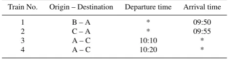
Table 2 Example trains at the same platform
Train No. Origin – Destination Departure time Arrival time
1 B – A * 09:50
2 C – A * 09:55
3 A – C 10:10 *
4 A – C 10:20 *
Empty-running may be planned on non-passenger routes. This may either short-cut the journey, or to allow the unit to reach locations that passengers normally would not reach, e.g. depots, shunting tracks, cleaning and refueling locations.
In an automatic scheduling process, empty-running is usually planned using a predefined collection of empty-running journey time allowances between location pairs. There may also be time zones when empty-running is prohibited. At the end of the scheduling process, empty-running trains are planned in detail and ensured to be conflict free. At that stage, it is possible that some adjustments to the schedule are required because some empty-runnings may turn out to be infeasible.
2.1.4 Shunting movements and station infrastructure
The linkage between an arriving train and a departing train sometimes may only be accomplished by certain shunting movements. Railwayshuntinggenerally refers to empty-running movements betweenplatforms,sidingsanddepotsduring a linkage. Shunting plans enable units to be delivered to the right location at the right time without causing blockage to each other. The length of empty running required varies between different types of shunting movement. Whereas the arrival and departure platforms for trains are usually assigned at the timetable planning stage, the assign-ment of which sidings or depots the units will be shunted to are only planned at the unit diagramming stage. Since depot shunting usually occurs before or after an idle period for the unit, it is generally less constraining on unit scheduling.
A distinctive feature that makes rolling stock scheduling different from road (e.g. bus) vehicle scheduling is that movements of rolling stocks are strictly restricted by tracks and other railway infrastructures like platforms and sidings, giving additional problems such as unit blockage or hitting platform or siding capacity restrictions. In some literature, blockage is also known ascrossing(Freling et al (2005), Kroon et al (2008)). Other issues may also be relevant to shunting, for example, compatibility between traction type and platform/siding/depot.
To illustrate how crossing can invalidate a unit diagram derived solely based on timetable and fleet information without station infrastructure detail, consider a sim-ple examsim-ple. Table 2 gives a timetable of four trains. Suppose at station A all the four trains have been assigned to the same long platform, where the tracks are bidirec-tional. There are two train units available each with sufficient capacity for any of the trains. Suppose Unit I can only serve Trains 1, 3 and 4, while Unit II can serve Trains 2, 3 and 4.
To C To B
Unit II Unit I
Arr 9:55 from C
Dep 10:20 to C Arr 9:50 from BDep 10:10 to C 1
3
2
4
B-A C-A
A-C A-C
Platform 7 of A
Fig. 1 Station blockage with the FIFO solution (i)
To C To B
Unit II Unit I
Arr 9:55 from C
Dep 10:10 to C Arr 9:50 from BDep 10:20 to C 1
3
2
4 B-A C-A
A-C A-C
Platform 7 of A
Fig. 2 A feasible solution (ii)
(i) Unit I: Train 1−→Train 3, Unit II: Train 2−→Train 4;
But solution (i) is infeasible because when departing at 10:10, Unit I will be obstructed by Unit II whose departure time is 10:20. It would be easy to see that an alternative feasible solutions exists:
(ii) Unit I: Train 1−→Train 4, Unit II: Train 2−→Train 3.
The two solutions are illustrated in Figure 1 and 2, showing how train directions and station infrastructure can adversely affect the results if the scheduling process does not take them into consideration.
Within the train unit scheduling process, train sequencing and fleet assignment based on timetable, fleet and route knowledge can be regarded as network wide high-level planning. On the other hand, shunting movements (including null shunting) based on detailed infrastructure and train direction knowledge belong to a lower level planning involving platforms, sidings and depots. High-level planning alone may result in problems such as crossing, which would hinder the solutions from be-ing operable; but then, incorporatbe-ing every detailed infrastructure information into the scheduling method will lead to an extremely huge-sized optimization problem intractable to solve. Therefore, a two-phase approach is preferred as a compromise, which is to be discussed in Section 4 and 5.
3 Literature review
3.1 Train sequencing and fleet assignment problem
coupling, the weak knapsack constraints for passenger demand satisfaction are dealt with by explicitly finding relevant convex hulls in 2-dimensional spaces.
Alfieri et al (2006) consider a similar scenario as Schrijver (1993) for NS Reizigers; the objective is to minimize the total number of train units used plus carriage-kilometers. Additional considerations are given in unit permutation and shunting time buffering. Some detailed infrastructure-related problems such as shunt crossing are ignored at this planning stage. The transition graph concept is introduced.
Fioole et al (2006) describe a similar model and instance as Alfieri et al (2006) with additional considerations on train splitting and joining. Peeters and Kroon (2008) describe a similar model and instance as Alfieri et al (2006) with a specialized solver employing branch-and-price.
Mar´oti (2006) proposes generalized models of the above works in the Netherlands in his PhD thesis.
Cacchiani et al (2010) propose an integer multicommodity flow ILP model for some local train unit scheduling problems. The LP-relaxation is solved by column generation and a diving heuristics is used for finding integer solutions and speeding-up the process. Taking advantage of the local instances where no more than two units are coupled (from many potential types), the weak knapsack constraints per train for demand satisfaction are overcome by computing a dominant set of a polytope defined over another space. This model is applied for real-world instances of up to 600 trains. Location restrictions and time allowances for coupling/decoupling, type-type compatibility and shunting resolutions are not considered.
3.2 Railway shunting problem
Freling et al (2005) propose a two-phase approach to solve the railway shunting prob-lem at a station within a 24-hour horizon. The method is based on a set-partitioning ILP model with each column corresponding to a feasible assignment plan for a siding. Both single (FILO) and double (free) sidings are considered. It prevents overcapac-ity and crossing at each siding, and also minimizes unnecessary coupling/decoupling activities. The instances tested have up to about 80 train units to be parked at 19 sid-ings. This two-phase approach gives near-optimal solutions, with small gaps to global optimality.
Kroon et al (2008) later propose another approach for the same railway shunting problem as in Freling et al (2005), where an integrated model (and three of its vari-ants) is devised such that matching and assigning is processed together, hence global optimality is guaranteed. To avoid a possible huge number of crossing constraints, maximal cliques and comparability graph techniques are used.
3.3 Generate-and-select and PowerSolver
Generate-and-Select(GaS) approach in crew scheduling, in which the column gener-ation process only brings in new columns within a pre-generated very large collection of columns. Apart from the advantage of reducing computation associated with solv-ing pricsolv-ing subproblems, a reasonably sized selection of the pre-generated columns could also be made for the branch-and-bound process. Kwan and Kwan (2007) fur-ther propose a hybrid method calledPowerSolverto solve very-large-scale train crew scheduling problems. PowerSolver uses an iterative heuristics to control the size of the problem instance in each execution of its core algorithm (GaS with set-covering ILP) such that the ILP solver works comfortably due to the reduced problem size. Ini-tially, the controlled problem instance is a crude simplification of the original problem instance; it is then refined and converges to containing the crucial features in a com-pact form over a number of iterations. A mechanism to ensure that new solutions would not be worse than the current best is embedded, thus the results would con-verge to a near-optimal one within a relatively short time. PowerSolver is now part of the TrainTRACS system (Fores et al (2002); Wren et al (2003)) and is proving successful by many UK transport operators who are now routinely using it. A sim-ilar approach to PowerSolver could be applied in train unit scheduling and will be discussed in later sections.
4 A fixed-charge multicommodity flow model for the first phase
Considering that the unit scheduling problem would be huge and intractable if all detailed infrastructure constraints are to be considered at once, a two-phase approach is proposed.
The first phase for train sequencing and fleet assignment uses an integer FCMF model similar to Cacchiani et al (2010). But the model is more comprehensive in modeling real-world conditions and constraints typical of UK railway operations, es-pecially the coupling/decoupling location restriction and time allowances, and type-type compatibility enforcement. The aim is to produce solutions that are near to being fully operable.
The second phase for station shunting finally determines the finer operational plan details in a station-by-station manner. For example, precise track and platform lay-out constraints are considered for determining the best operable shunting movement plans. It will be described in Section 5.
4.1 Model description
The integer FCMF model is based on a framework ofdirected acyclic graph(DAG) representing trains and their relations. A generic DAGG= (N,A)consists of nodes and directed arcs such that no cycle exists.
In this framework, the majority of nodes represent the trains in the timetable, thus are calledtrain nodes, denoted byNe. In addition, asource node0 and asink node
NB+⊆Nefor arrival locations. There are three kinds of arcs in the DAG, namely sign-on arcs,sign-off arcsandlinkage arcs. A sign-on arc starts from the source node and ends at a train node; a sign-off arc starts from a train node and ends at the sink node. Generally all train nodes have a sign-on arc and a sign-off arc. We denote the set of all sign-on/off arcs byA◦. A linkage arca∈Aelinks two train nodesiand j(a= (i,j)), representing a potential link, with a sufficient time gap, such that after serving train
ia unit can continue to serve train jas its next task. Note thatA=A◦∪Ae. We use δ−(j)to denote all arcs that terminate at node j, andδ+(j)for all arcs that originate
from node j; and useE to represent the set of all arcs implying empty-running. A
path p∈Pin the DAG is defined as a sequence of nodes starting from the source
to the sink such that from each of its nodes there is an arc to the next node in the sequence. A path represents a daily workload (a diagram) for a unit. In addition,Pj
andPadenote the sets of paths passing through node jand arcarespectively;Jpand Aprepresent the sets of nodes and arcs in pathprespectively.
For the fleet, we denoteTthe set of all unit types. In order to deal with type-route compatibility, type-graphsGt (also DAGs) representing routes each unit typet∈T
is able to serve are constructed based on the above complete DAGG. All entities in the type-graphsGtcan be symbolized by adding atsuperscript in the corresponding notations of the complete DAGG, e.g.Pt refers to the set of all paths in type-graph
Gt. We useFto represent the set of all unit families, andFj the set of families that
can serve train j.
There are three kinds of decision variables.Path variable xp∈Z+,∀p∈Pt,∀t∈T
is used to indicate the number of units used in pathpfromGt. For each train and the
families serving it, we settrain-family variable yfj ∈ {0,1},∀j∈Ne,∀f ∈Fj, to
in-dicate whether a train j is served by any units from family f.Blockflow variable za∈ {0,1}is used to indicate whether an arca= (i,j)∈Ais used. It corresponds
to a block of units that remains coupled together during two consecutive trains i
and j.zais used to forbid coupling/decoupling at banned locations, calculate time
consumed by coupling/decoupling operations, as well as eliminate unnecessary cou-pling/decoupling activities.
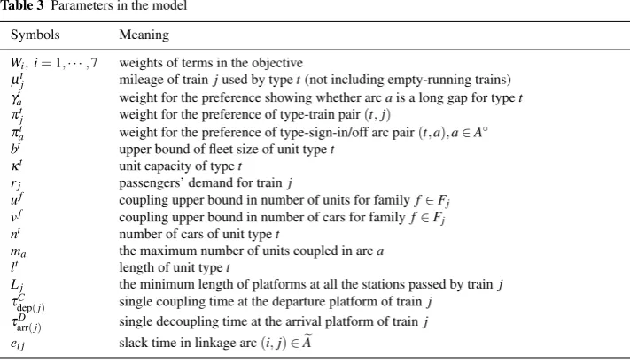
Finally, Table 3 describes the parameters used in the model.
4.2 Path formulation
If column generation is to be used for a multicommodity flow problem, generally a path formulation would be preferred than an arc formulation as the master problem, although the bound given by LP-relaxations of both are the same (Geoffrion (1974); Barnhart et al (1998); Cook et al (1998); Cacchiani et al (2010)). We choose an LP-relaxation rather than a Lagrangian LP-relaxation as nowadays a state-of-art simplex solver can be more efficient than a subgradient method.
Table 3 Parameters in the model
Symbols Meaning
Wi,i=1,· · ·,7 weights of terms in the objective µt
j mileage of trainjused by typet(not including empty-running trains)
γt
a weight for the preference showing whether arcais a long gap for typet
πt
j weight for the preference of type-train pair(t,j)
πt
a weight for the preference of type-sign-in/off arc pair(t,a),a∈A◦ bt upper bound of fleet size of unit typet
κt unit capacity of typet rj passengers’ demand for trainj
uf coupling upper bound in number of units for familyf∈Fj vf coupling upper bound in number of cars for familyf∈Fj nt number of cars of unit typet
ma the maximum number of units coupled in arca lt length of unit typet
Lj the minimum length of platforms at all the stations passed by trainj
τC
dep(j) single coupling time at the departure platform of trainj
τD
arr(j) single decoupling time at the arrival platform of trainj ei j slack time in linkage arc(i,j)∈Ae
min
x,z W1
∑
t∈Tp∑
∈Ptxp+W2
∑
t∈Tj
∑
∈Net∑
p∈Ptj
µtjxp+W3
∑
t∈Ta
∑
∈Etp∑
∈Pt axp
−W4
∑
t∈Ta
∑
∈Aet∑
p∈Pta
γatxp−W5
∑
t∈Tj
∑
∈Net∑
p∈Ptj
πtjxp
−W6
∑
t∈Ta∈
∑
(A◦)tp∑
∈Pt aπt
axp+W7
∑
a∈A za
(1)
subject to
∑
p∈Ptxp≤bt, ∀t∈T; (2)
∑
t∈Tp∑
∈Ptj
κtxp≥rj, ∀j∈Ne; (3)
∑
t∈fp∑
∈Ptj
xp≤ufyfj, ∀j∈Ne,∀f∈Fj; (4)
∑
t∈fp∑
∈Ptj
ntxp≤vfyfj, ∀j∈Ne,∀f ∈Fj; (5)
∑
f∈Fjyfj =1, ∀j∈Ne; (6)
∑
t∈Tp∑
∈Ptj∑
t∈Tp∑
∈Pta
xp≤maza, ∀a∈A; (8)
τD
arr(i)
(
∑
a∈δ+(i)za−1
) +τC
dep(j)
(
∑
a∈δ−(j)za−1
)
≤ei j, ∀(i,j)∈Ae:i∈/NB+,j∈/NB−;
(9)
∑
a∈δ−(j)za=1, ∀j∈NB−, (10a)
∑
a∈δ+(j)za=1, ∀j∈NB+; (10b)
xp∈Z+, ∀p∈Pt,∀t∈T, (11a)
yjf ∈ {0,1}, ∀j∈Ne, ∀f ∈Fj, (11b)
za∈ {0,1}, ∀a∈A. (11c)
4.2.1 Objective function
The objective (1) is formed by seven terms. The first term minimizes the total num-ber of units used. The second term minimizes the total passenger train unit-mileage, whereµt
jis the mileage of train j∈Ne used by single unit of typet. The third term
minimizes the total number of empty-running trains. The fourth term encourages in-sertion of long gaps in unit diagrams such that maintenance can be realized whereby. Parameterγt
a=0 if arca does not imply a long gap or this gap is not suitable for
typet;γt
a>0 if arcacontains a long gap that is suitable for typet. There are also
preferences among positive values ofγt
aas some long gaps are more suitable for type tthan others. The fifth term encourages type-train (route) preferences, whereπt
j≥0
is a preference weight for a type-train pair(t,j): the higher the more suitable. The sixth term encourages sign-on/off arc preferences (usually related to home depots) for each type of units, whereπt
astands for a preference parameter for a type/sign arc
pair(t,a): the higher the more suitable. Notice if a certain typet is not suitable for a sign-on/off arc, this arc will not have been inserted intoGt in the first place. The seventh term minimizes the total number of blocks, leading to minimization of the total number of coupling/decoupling activities; it also partly driveszato desired
bi-nary values. Notice the appearance ofzain the objective categorizes this model into
a fixed-charge multicommodity flow type.
4.2.2 Constraints
Constraints (2) ensure deployed number of units for each type within its upper bound. Constraints (3) guarantee satisfaction of capacity demand for each passenger train. Constraints (4) and (5) calculate each family-train indicator variable as well as re-stricting the possible coupling combinations in terms of both the total number of units and the total number of cars. Constraints (6) allow only one family to serve a train.
Notice (4), (5) and (6) together will ensure thatyfj = {
1,∑t∈f∑p∈Pt jxp>0
0,∑t∈f∑p∈Pt jxp=0
,∀j∈
e
N,∀f ∈Fj. Constraints (7) are platform length constraints. Constraints (8)
calcu-late blockflow variables. Notice as the sum of blockflow variables is minimized in
the objective, the relationza=
{
1,∑t∈T∑p∈Pt axp>0
0,∑t∈T∑p∈Pt axp=0
,∀a∈Ais guaranteed.
Con-straints (9) are to ensure time allowance validity for coupling/decoupling if it is al-lowed. Constraints (10) are to forbid coupling/decoupling at banned locations. Finally (11) gives the variable domain.
Notice some intuitive simplification will apply, e.g., trains whose platform lengths are long enough do not need constraints (7), and the linkage arcs whose slack time is long enough and relevant locations allow coupling/decoupling, constraints (9) can also be omitted. For those trains only allowing compatible types to serve, train-family variablesyfj and constraints (6) associated with them can be omitted, and relevant coupling upper bound constraints (4) (5) can also be simplified. And so on.
5 A multidimensional matching model for the second phase
5.1 Station element representation and model description
5.1.1 Arrival and departure units
The first phase provides a tentative schedule based on which the second phase op-erates within the scope of each individual stationσ ∈Σ. The first phase fixes the unit-type assignment to each arrival and departure train, e.g., “train 1E08 is served by one British Rail Class 171/7 and one British Rail Class 171/8 units”. We can thus define a set ofarrival unitsand a set ofdeparture unitsfor a day’s operation at each stationσ, asu1,u2,· · ·,un∈Uσandv1,v2,· · ·,vn∈Vσ respectively. The first phase
also results in a tentative assignment of a next departure unit for every arrival unit, and these assignments may have to be modified by the second phase because of op-erational conflicts at the station. Here we assume empty running trains have been inserted by the first phase and|Uσ|=|Vσ|=n. Sign-on/off trains from/to a home depot can be dealt with by slight adaptation. Exceptions, such as over-night units remaining at the station cannot invalidate this model as sign-on/off arcs regard this station as the source/sink node. For simplicity, we will omit the superscriptσin later part of this section as everything is clearly based on a single station, except where explicitly stating the station is necessary.
– The train the unit belongs to:T(u),T(v). Notice an arrival unit only belongs to one arrival train and a departure unit only belongs to one departure train. – The attributes due to its train: the arrival platform of an arrival unitP(u)and the
departure platform of a departure unitP(v); the arrival time of an arrival unitτ(u)
and the departure time of a departure unitτ(v). – The type of that unit:t(u),t(v).
Amatching between an arrival unit and a departure unit is used to represent a
linkage relation. A matching between twoconceptualarrival and departure units u
andvindicates they will bematerializedby being assigned to be the same unit. The first-step rule of how an arrival unitu can be matched with a departure unit vis: (a) Same type:t(u) =t(v); (b) the arrival time ofuis appropriately earlier than the departure time ofv:τ(u)≺τ(v).
Other linkage validity rules regarding shunting/coupling/decoupling times will be considered respectively in other ways. It is important to note that avalidmatching between a pair of arrival and departure units(u,v), u∈U,v∈V will correspond to one and only one linkage arc(T(u),T(v))∈Aein the DAG defined in the first phase. This linkage arc is called adominant arcof the matching pair.
5.1.2 Unit position
If a train is a coupled one, thepositionsof the units in the coupled formation are im-portant information. Since the first phase has not provided anything on unit permuta-tion for coupled trains, it has to be decided in the second phase. Letp∈Pu,q∈Qv
de-note positions and their possible choice sets for arrival unituand departure unitv re-spectively. For a unitu(orv) from a non-coupled train, its position is unique(|Pu|=1
or |Qv|=1); for a coupled single-type (homogenous) train, unit positions can be
pre-assigned based on the first phase result in an arbitrary order, leading to|Pu|=1
or |Qv|=1 as well; for a coupled multi-type (heterogenous) train where different
permutations can have essentially different results, a decision has to be made from
p∈Pu,q∈Qv,|Pu|>1,|Qv|>1. Therefore, the above matching has to be further
modified within apositionedpair of(u,p)and(v,q)such that a plan(u,p,v,q),u∈
U,p∈Pu,v∈V,q∈Qvhas to be made.
u1 u2 front rear
v3 v4
rear front
Fig. 3 A matching in a dead-end platform scenario
u1 u2
v3 v4
rear front
Fig. 4 A matching with coupling in a FIFO scenario
FIFO track, thenu1can only be coupled at the rear ofu2, which indicatesu1can only be matched withv3andu2withv4. Cases in coupled multi-type trains will be more complicated.
5.1.3 Parking berths
Generally speaking, there are three possible kinds of shunting plans at each linkage arc: to let the unit continue to serve the next train within the platform area (short time gap linkage), to put the unit to a siding temporarily until it is needed for the next train (medium time gap linkage) and to put the unit to a nearby depot until it is needed for the next train (long time gap linkage). Here we denoteparking berthsas
b∈B:={0} ∪S∪Dwhere 0 refers to a dummy parking berth representing platform
stay,Sthe siding set andDthe depot set.
For a positioned pair of arrival and departure units(u,p,v,q),u∈U,p∈Pu,v∈ V,q∈Qv, the possible choice for parking berth types (dummy, siding or depot) is
dependent on the relevant time gap length of its dominant linkage arc(T(u),T(v)). A dummy berth is only imaginary, i.e. the unit stays put. However, if the parking berth turns out to be a siding or a depot, usually there are a number of sidings or depots available for a unit to be shunted to. We denote the possible parking berths for a pair of positioned units(u,p,v,q)asB(u,p,v,q).
5.1.4 Parking methods
a depot after an empty-running trip. This is because such movements are usually infrequent with sufficient time for resolving any conflicts that might arise.
Here we define the parking method m∈M(u,p,v,q,b)for a pair of positioned units(u,p,v,q)with its parking berthb∈B(u,p,v,q)as possible ways of how this unit arrives at and leaves its arrival platformP(u), comes to and leaves its parking berthb, and then comes to and departs from the departure platformP(v). For a pair yielding a dummy or a depot parking berthb∈ {0} ∪D, the ways coming to and leavingbis omitted as a default “00”.
Here is an example of such a parking method withb=0 and a null-shunting:
m= [LR,00,LR], which means arriving from the left and departing from the right, at the same platform without any shunting. Another example of a parking method involving a double (free) siding shunting with re-platforming:m= [LR,RL,LL]which means:
– at the arrival platform: arriving from the left and leaving from the right (to a siding);
– at the siding: coming from the right and leaving from the left (to the departure platform);
– at the departure platform: coming from the left and departing from the left.
Parking methods are determined by various factors, e.g. train directions, plat-form, unit position, siding, depot and overall layout relations, plus possible engi-neering and operational regulations. Usually when(u,p,v,q,b)is fixed, the resulting
M(u,p,v,q,b)would have a very small number of candidate methods. Especially when the parking berth is a dummy one, a single (FILO) siding or a depot, the possi-ble parking method is very likely to be unique.
5.1.5 Shunting plans and conflicts between a pair of shunting plans
The second phase shunting problem is defined as
At each stationσ∈Σ of the rail network, give each arrival unit u∈U a position
p∈Puand assign it to a departure unit v∈V with position q∈Qv, via a parking
berth b∈B(u,p,v,q)and with a parking method m∈M(u,p,v,q,b)such that
1. Each matching pair(u,v)implies a dominant linkage arc relation(T(u),T(v))∈
e
A;
2. Each positioned pair(u,p,v,q)is operationally feasible for connecting T(u)and T(v);
3. No crossing occur at platforms or sidings; 4. No overcapacity occur at any sidings or depots;
5. No breaking on any other temporal, spatial, engineering or operational rules that makes the overall plan inoperable.
A shunting plan can be expressed as a 6-tuple (u,p,v,q,b,m), u∈U,v∈V,
(T(u),T(v))∈Ae, p∈Pu,q∈Qv,b∈B(u,p,v,q),m∈M(u,p,v,q,b)representing
u1 u2 : : un v1 v2 : : vn 0 s1 s2 : : S|S| d1 d2 : : d|D|
L L L
L L L L L L R R R R R R R 0 0 0 0 0 0 0 0
Fig. 5 An illustration of shunting plans
specific arrival unitucan be written asΠu, the same forΠvfor a specific departure
unitv. Fig.5 gives an illustration of the concept of shunting plans (unit positioning is not depicted).
All the possible shunting plans can be pre-computed based on input data of sta-tion informasta-tion and the first phase results before the second phase begins. With a shunting plan(u,p,v,q,b,m)timings can be determined for the unit leaving the ar-rival platform, coming to the parking berth, leaving the parking berth and coming to the departure platform. Also, the following parameters are known from station layout knowledge.∆ τu: time duration at the arrival platformP(u);∆ τub:
shunting/empty-running time from platformP(u)to parking berthb;∆ τbv: shunting/empty-running
time from parking berthbto platformP(v);∆ τv: time duration at the departure
plat-formP(v). Then, the attributes of a shunting plan(u,p,v,q,b,m)include:
– All attributes inherited from its arrival and departure units, including traction types, trains, positions and platforms;
– At the arrival platform P(u): arrival time τ(u), leaving time λ(u):=τ(u) +
∆ τu, which forms a time windowat the arrival platform:Wu(u,p,v,q,b,m):=
[τ(u),λ(u)];
– At the departure platformP(v): coming time:χ(v):=τ(v)−∆ τv, departure time
τ(v), which forms a time window at the departure platform:Wv(u,p,v,q,b,m):=
[χ(v),τ(v)];
– At parking berth b: coming time χ(b):=λ(u) +∆ τub, leaving time λ(b):=
χ(v)−∆ τbv, which forms a time window at the parking berth:Wb(u,p,v,q,b,m):=
[χ(b),λ(b)].
Although a shunting plan may be self-consistent in operation, the interaction be-tween shunting plans may still make the overall schedule inoperable. We denote a
pre-computed as input data for the second phase. We use
Π†(π) ={π′|π′†π,∀π′∈Π}
to denote the set of all shunting plans that have a conflict relation with shunting plan πand
C={(π,π′)|π†π′,∀π,π′∈Π}
the set of all conflicting shunting plan pairs.
5.2 Model formulation
If the unit-type contents of each train derived from the first phase result remain un-changed, the fleet size and most other terms in the objective function (1) will remain unchanged even if the second phase modifies the first phase results by resetting some matching pairs. The second phase can be regarded as rematching arrival units with departure units at each station, or from a diagram’s point of view,swappingtrains between the diagrams derived from the first phase. Therefore the global optimality given by the first phase will be mostly preserved.
We denote the set of all dominant arcs pertaining to stationσasAσ. As for each valid shunting plan(u,p,v,q,b,m),(T(u),T(v))corresponds to a unique dominant arca∈A, we thus denote the arc corresponding to shunting planπ as a(π), i.e. if π = (u,p,v,q,b,m), thena(π) = (T(u),T(v))∈Aσ. Then, after the path variables
xp,p∈Pt,t∈T from the first phase results have been transformed into arc variables
byxa=∑p∈Pt
axp,∀a∈A
t,t∈T, it is possible to assign costsc
πto each shunting plan
π∈Π according to the following rule:
(i) If first phase resultxa(π)>0, thencπ=0;
(ii) If first phase result xa(π) =0, then cπ>0 and can be set according to some
preferences (e.g. traction type / parking berth).
By setting the above shunting plan costscπ and minimizing ∑π∈Πcπxπ, where
xπ∈ {0,1}indicates whether to use a shunting planπ∈Π, it ensures that if the part
of first phase result related with stationσ does not cause any conflicts at all, it will be exactly retained after the second phase.
Similar as in Kroon et al (2008), it is desirable to have each siding serving as few types of unit as possible, yielding more flexibility and robustness. There is no such a need for platforms or depots. We denoteytb,b∈S,t∈T as a binary variable indicating whether at least one unit of typetis parked at sidingb, and try to minimize ∑t∈T∑b∈Sytb.
Similar as in the first phase, it is possible to introduce binary blockflow vari-ablesza,a∈Aσ indicating whether an arca is used, which are used for forbidding
coupling/decoupling at banned locations, calculating coupling/decoupling time dura-tions at permitted locadura-tions and eliminating unnecessary such operadura-tions. We denote the set of all shunting plans pertaining to arce∈AσasΠe, i.e.Πe:={π|a(π) =e}.
Thenza=
{
1,if ∑π∈Πaxπ>0
0,if ∑π∈Πaxπ=0
Thus, the second phase model:
min
x,y,z W1
∑
π∈Π
cπxπ+W2
∑
t∈Tb
∑
∈Sytb+W3
∑
a∈Aσ
za (12)
subject to
∑
π∈Πu
xπ=1, ∀u∈U; (13)
∑
π∈Πv
xπ=1, ∀v∈V; (14)
xπ≤yt(b(ππ)), ∀π∈Π :b(π)∈S; (15)
xπ≤za(π), ∀π∈Π; (16)
∑
a∈δ−(j)za=1, ∀j∈Neσ; (17a)
∑
a∈δ+(j)za=1, ∀j∈Neσ; (17b)
τD
arr(i)
∑
a∈δ+σ(i) za−1
+τC
dep(j)
∑
a∈δ−σ(j) za−1
≤ei j, ∀(i,j)∈Aeσ; (18)
xπ+
1
|Π†(π)|
∑
π′∈Π†(π)
xπ′≤1, ∀π∈Π :Π†(π)̸=∅; (19)
lt(π)xπ+
∑
π′:Wb(π′)∩Wb(π)̸=∅
lt(π′)xπ′ ≤Lb(π), ∀π∈Π:b(π)∈S∪D; (20)
xπ∈ {0,1}, ∀π∈Π; (21a)
ytb∈R+, ∀b∈S,∀t∈T; (21b)
za∈R+, ∀a∈Aσ. (21c)
Constraints (13)–(14) match each arrival unit to a unique departure unit via a unique parking berth by a unique parking method, and the same for each departure unit. Similar concept for ensuring each position in coupled multi-type trains to be occupied by one and only one unit has been encapsulated implicitly by conflict sets.
Constraints (15) calculate the siding-type variables, where t(π) is the traction type implied by shunting planπ andb(π)is the parking berth of planπ. Notice here we use a disaggregated formulation with many constraints (=|Πb(π)∈S|) rather than
an aggregated formulation with less constraints, e.g. a multiple variable lower bound (MVLB) (Ciriani et al (2003)) like
1 |Πt
b|π
∑
∈Πt bxπ≤ytb, ∀b∈S,∀t∈T, (22)
whereΠt
bis the set of shunting plans implying a typet to be shunted to a berthb.
The stronger disaggregated formulation (15) will generally give a much tighter LP-relaxation than (22), and also let yt
b be only continuous while functioning binary.
The side effect from excessive number of constraints in (15) can be neutralized if a column-and-dependent-row generation approach is used.
Constraints (16) calculate the blockflow variables for each dominant arc pertain-ing to stationσ. Similar as in (15), we use a strong formulation rather than an MVLB formulation.
Only one from Constraints (17) and (18) will appear for a specific station σ, depending on whether coupling/decoupling is banned atσ (use (17)) or allowed (use (18)).Neσ is the set of train nodes related with stationσ.
Constraints (19) prohibit conflicts between each pair of shunting plans. Note that a generic conflict (or crossing) exclusion formulation such as
xπ+xπ′≤1, ∀(π,π′)∈C (23)
will give a huge number of constraints leading to computational difficulty (e.g. Model 1 in Kroon et al (2008)). Some successful remedy methods, for instance, taking ad-vantage of clique inequalities or comparability graphs (e.g. Model 2 and 2a in Kroon et al (2008)) are not suitable for the current problem, where the concept of conflict is based on a more complex context concerning positions, platforms, sidings and com-bined parking methods. Here we propose another remedy method as in (19). Com-pared with (23), the number of constraints has been significantly reduced, as usually |C| ≫ |Π|. Notice the number of constraints will be further reduced if a column-and-dependent-row generation approach is used.
Constraints (20) prohibit overcapacity for each siding and depot berth, wherelt(π)
is the capacity consumed by typet(π)implied from shunting planπ, andLb(π)is the total capacity of parking berthbimplied from planπ. From observations of the man-ual scheduling process, feasible berthing plans can always be found in a station-by-station manner. Moreover, berth capacity would have been satisfied at the preceding timetabling stage, i.e. the input timetable determines the main unit flows on stations at certain times and places, as train unit scheduling only assigns units to predetermined trains.
6 Solution approaches
6.1 Pre/dynamic column generation
We first give a short discussion on ways columns are generated in a generic column generation process, which seems has not been given much attention in the literature.
Generally, if a generic column generation approach is to be used, except the ini-tial columns providing a feasible solution to trigger the subsequent process, all new columns to be added to the restricted master problem (RMP) have to be generated from some methods. There are usually two ways for generating them. The first one is to generate dynamically from subproblems until no good candidate is available and theoretically the solution will be guaranteed global optimal. However, this approach has two major disadvantages, both due to the dynamic nature how new columns are generated. One is the difficulty in satisfying sophisticated rules imposed on each col-umn; the other, arising in integer programs solved by branch-and-bound (BB), is that dynamically generated columns may have some properties inconsistent with the cur-rent branch status (Barnhart et al (1998)). These lead to the need for designing very complicated subproblems or ad-hoc branching strategies to exclude invalid candi-dates. Constrained shortest path subproblems for crew scheduling (Irnich and De-saulniers (2005)), generalized assignment problems (Savelsbergh (1997)) and single-path multicommodity flow problems (Barnhart et al (2000)) are well-known exam-ples.
Alternatively, it is possible to perform a pre-generation beforehand trying to ex-tract the essence of all possible candidates into a pot, and then carry on subse-quent column generation process only based on this pot. Candidates are priced out by merely calculating and comparing their reduced costs, and unlike in dynamic-generation, it is convenient and flexible to addseveralcandidates to the RMP from the same decomposed subproblem. Moreover, the above two disadvantages from dynamic-generation are unlikely to occur in this approach, making it more prefer-able for solving very large-scale complex problems, especially when sophisticated rules are imposed on individual columns. Its disadvantage is theoretically it cannot always guarantee global optimality, as the solution only converges to a local optimum with respect to the pre-generated pot. Examples of this style include Fores (1996) for bus driver scheduling, Kwan (2004) for large-scale crew scheduling and Hennig et al (2012) for maritime transport routing.
6.2 A hybrid approach for the first phase
simplify-ing those knapsack constraints by similar methods as in the above literature, and we have to keep them when solving the model.
We find that, as also observed in Cacchiani et al (2010), exact methods would be incapable of handling very large problem instances. Here we propose a Size Limited Iterative Method (SLIM) based on hybridization of an exact method (a branch-and-price integer linear programming (ILP) solver) and a heuristic framework.
6.2.1 A branch-and-price approach for the exact solver
A branch-and-price (Barnhart et al (1998)) approach is used for the exact ILP solver. Unlike in crew scheduling, the rules imposed upon each unit diagram are not very complex. Thus we use dynamic column generation where the subproblem is a generic shortest path problem. Although there are three kinds of variables, as the last two are solely determined by the path variables, we only price out path variables.
Let βt ≤0,ρ
j ≥0,φjf ≤0,ψjf ≤0,λj ≤0,ζa≤0 be the dual variables from
constraints (2), (3), (4), (5), (7), (8),f(p)be the family of pathp∈Pt,t∈T, andcp= c0p+∑j∈Jpcj+∑a∈Apcabe the generalized cost ofpin the objective (1) consisting of
three parts (relevant with nodes, relevant with arcs and irrelevant with any of them). The reduced cost ofpfromGtis,
¯
cp=c0p−βt+
∑
j∈Jp(
cj−κtρj−φjf(p)−n tψf(p)
j −l
tλ j
) +
∑
a∈Ap
(ca−ζa), (24)
finding the smallest value of which can be regarded as a shortest path problem with train nodej∈Nethe weightcj−(κtρj+∑f∈Fjφ
f
j+nt∑f∈Fjψ f
j+ltλj), arca∈Athe
weightca−ζa, plus a source-sink weightc0p−βt. There are|T|subproblems from
Dantzig-Wolfe decomposition.
As for the branching strategy, it is a usual way to branch on the corresponding compact formulation while working on the extensive formulation (Villeneuve et al (2005)). This means we can branch on arc variables while performing the column generation with path variables. However, we find it difficult to design an efficient branching method with respect to arc variables by only deleting certain columns with-out adding explicit branching constraints, which is to be preferred. This is because the arc variables are integral rather than binary; moreover, each type can use multiple paths in the final integer solution, unlike the case in Barnhart et al (2000) where each commodity takes one and only one path. We here propose a mixed branching strat-egy consisted of two branching rules, namelytrain-family branchingandarc variable
branching.
Train-family branching The main idea of train-family branching is to check the LP
relaxation solution and select a train jthat is covered by more than one family, say families f1,f2,· · ·,fk(kis usually not a large number). Then we formk+1 branches
– For the firstkbranches 1,· · ·,k, say at a branchi∈ {1,· · ·,k}, only the family
fi is allowed to serve train j. To achieve this, in the RMP, all paths indicating
any families inFj\ {fi}serving jare deleted. Moreover, to prevent subproblem
regeneration in a branch-and-price framework, in the shortest path problem of typet whose family is not fi, node j is deleted from the shortest path network.
Variablesyfj and constraint (6) for train j can then be removed from the RMP, and constraint (4) (5) can also be modified according to which family serves that train.
– In the last (k+1)th branch, if |Fj\ {f1,· · ·,fk}| ≥1, then we forbid families f1,· · ·,fk to serve train j, which can be realized by similar path/node
delet-ing ways as described above, and there is no removal/modification of related variables/constraints unless|Fj\ {f1,· · ·,fk}|=1; ifFj={f1,· · ·,fk}, then the
(k+1)th branch is no longer needed.
Notice this branching rule does not add any extra constraints to the RMP. It actually reduces the number of columns in the RMP and the network scale of the shortest path subproblems, which effectively divides the search space and forces the train-family variables to be integral.
Arc variable branching The train-family branching is the first choice in the
branch-and-bound tree. However, when all trains are served by single families, this branching rule cannot be used any more. At this moment, the second branching rule, arc vari-able branching, will be invoked. This rule detects fractional arc varivari-ables from the result of the RMP LP relaxation byxt
a=∑p∈Pt
axp, and branches over this arc by
explicit branching constraints. We use a constraint branching rule similar as the one for integer multicommodity flow in Alvelos (2005), i.e. on one branch, add constraint ∑p∈Pt
axp≤ ⌊x t
a⌋, and on the other branch, add constraint∑p∈Pt axp≥ ⌈x
t
a⌉. As all those
constraints are associated with arcs, the structure of shortest path subproblem can be kept by adding arc weights from dual variables of those constraints; invalid path gen-eration is also prevented straightforwardly. We currently first select on the arcs with most fractional values to branch but find it is not very efficient. It is also a good idea to first branch on fractional arcs at peak times, as is used in Schrijver (1993). For node selection, a best-first strategy is used, which will always provide us a global lower bound.
The second rule will only be triggered when the first rule cannot be used. Notice after the second rule is used, there may be some trains served by multiple families again, and thus the first rule will be called again until all trains are again covered by single families, and the switch to the second rule, and so on.
6.2.2 A size limited iterative method
supplementary methods, the problem instance will be adjusted to derive a different new instance that would not yield a worse result, and to be solved again by the exact solver. This process will be repeated until no significant improvement. The problem instance compaction retains all the train trips, i.e. the method does not subdivide the problem instance into small separate subproblems.
Size reduction on problem instance can be achieved by mainly two methods:
(i) Simplifying permitted types available for trains such that no type incompatibil-ity can occur;
(ii) Pre-sequencing some trains intosuper-trainsso that they will each be scheduled as an integral block.
The first method eliminates a large number of variables and constraints used for en-suring type-type compatibility. As this heuristics proceeds, types that have once been deleted from a train will have the chance to be added back based on certain mech-anisms to allow solution improvement. The second method significantly reduces the number of “trains” by pre-sequencing them into super-trains. According to the cur-rent solution status, super-trains would be reformed between iterations.
Outline of SLIM
1. Associate trains with a subset of permitted types.
2. Form a set of super-trains each replacing the original trains in the sequence. 3. Solve the reduced problem instance derived using the ILP solver. If it is not the
first result obtained and there is no improvement on the objective for a predefined number of iterations, GOTO 7.
4. Copy the last problem instance to a new instance and then retain from the current best solution only the linkage arcs used.
5. Extend the search space by decomposing some super-trains and/or forming some new super-trains according to some defined criteria and make sure the resulting solution will be no worse than the current best solution.
6. Heuristically include more potential arcs into the problem instance, ensuring that the problem size is not exceeding a predefined upper limit. Go back to 3. 7. If the full set of permitted types is allowed for all trains, STOP. Otherwise, extend
the search space by gradually re-instating the full set of permitted types. Go back to 3.
6.3 A column-and-dependent-row with pre-generation approach for the second phase
Column-and-dependent-row generation A challenge for the second phase model, say if column generation is to be used, is the constraints based on columns (con-straints (15), (16), (19) and (20)), which will cause theoretical problems that make the column generation invalid. Simply speaking, if only a subset of columns are present in the RMP, then the rows corresponding to the missing columns will be also absent with their dual variables unknown, leading to incorrect reduced cost calculation, not to mention the primal feasibility is also no longer guaranteed. This is an interesting new research direction of column generation, and very few relevant literature can be found. The only focused research so far, is from Muter et al (2012), which gives a deep insight into it, and also proposes a solution approach for two-variable cases. We believe that it is possible to expand the method in Muter et al (2012) to some three-variable cases, as our second phase model. We will continue to focus on this special kind of column generation problem, and propose a column-and-dependent-row gen-eration approach for our model in the future.
Pre-generation and initial test We use a pre-generation approach for our
column-and-dependent-row generation. The complex rules imposed on individual shunting plans make it almost impossible to generate such candidate plans dynamically. All possible candidate shunting plans forming the set ofΠwill be pre-generated. Another major step beforehand is to construct the conflict setsΠ†(π)for each shunting plan π ∈Π. For efficiency reasons, an initial testing phase is used where only a set of columns corresponding to the first phase results (i.e. all the shunting plans with zero costscπ =0) is provided for the RMP. If those columns yield a feasible solution
for the second phase, then the process is stopped and optimality claimed. Otherwise, extra columns have to be added to construct an initial feasible solution and then the commence of a column generation process.
Heuristics Some heuristics speeding up the solution process can be also used, e.g.
the idea of utilizing homogenous sidings to get near-optimal solutions quickly (Kroon et al (2008)). Another direction to be explored is theorderhow stations are processed. Clearly different orders will very likely give different solutions, since solving a station will simultaneously fix some characteristics of arrival/departure units of other related stations, and it is not clear yet how to determine the order to improve the overall solution.
Branching Strategy A mixed branching system is to be used, inclduing: (i) branching
7 Computational experiments
7.1 Southern railway dataset
This research benefits from collaboration with Southern Railway, UK, which is a very large passenger train operator in the South of England. Each year, there are two timetables published. A full set of data for a timetable in December 2011, including their actual unit diagrams used, has been used for developing our models and for test-ing. The timetable concerned has over 2400 train trips on a typical weekday, and 11 different types of train units are in use. Furthermore, the network covered is extensive with numerous routes, stations and platforms. Hence, the setup and configuration for testing our models is in itself a very substantial ongoing task. Whilst some promis-ing results have been obtained, they still have to be carefully analyzed with Southern Railway. More comprehensive results therefore will be reported in a future paper.
Knapsack constraints The Southern Railway’s data has very complicated type-route
compatibility relationships, giving large numbers of unit types available for most of the trains (e.g. 7 types can serve the London Bridge – East Croydon route), mainly due to the use of four types of British Rail Class 377, which basically can run on any route. Moreover, Class 377/3 has a coupling upper bound of 4 units, and Class 377/1, 377/2 and 377/4 have a bound of 3 units. If using family generalization, the family Class 377 has an upper bound of 12 cars with various car number coefficients in the constraint. These features forbid us from using the knapsack constraint sim-plification method developed by Cacchiani et al (2010) (for a coupling upper bound of 2 units) for almost all trains. Thus we have to retain all knapsack constraints at this stage. Since Southern Railway cannot provide us with passenger demand data, all passenger demands per train (rj) are derived reversely from the Southern
Rail-way December 2011 diagrams. Notice this will not surely alleviate the difficulty of knapsack constraints, as the unit types other than the one used in the real diagrams also appear in the demand satisfaction constraints. Also, not all platform length con-straints are present in the experiments since complete data was not available when we did the testing.
Arc length In constructing the DAG network, there is a minimum and maximum
time restriction for linkage arc lengths, currently set to be 5 min and 720 min re-spectively. We are aware that setting the latter a much smaller value (e.g. 360 min) will significantly reduce the number of arcs, which dominates the number of rows in the formulation, while most of the “long” arcs will never be used. However, the need for long gaps for maintenance and off-peak depot berthing requires us to retain them. Typically there is a morning peak and an afternoon peak in the timetable, and between the two peaks it is preferred to have most of the units back to some nearby depots, and some of the units may be under maintenance operations during this idle time.
Empty-running trains We use existing empty-running trains extracted from the
route network information using a shortest path algorithm. There were originally some constraints for eliminating conflicting empty-running trains in the first phase formulation, but we finally discarded them for not further increasing the problem scale.
7.2 Branch-and-price solver design
The main purpose of our experiments is to verify the validity of the first phase model, rather than to solve the entire problem as a whole or to test our ad-hoc solver’s per-formance, which will be reported in continuing research. For all the experiments re-ported here, only the first phase is involved, and SLIM is not used. Notice we have to retain all knapsack constraints. We will first shortly describe some practical aspects of our branch-and-price solver used in the experiments.
7.2.1 Primal heuristics
We use a greedy heuristics to generate the initial columns for the column generation at the root node of the BB tree. The main rationale of this primal heuristics is to select the tightest arc (with respect to time) for linking the next train at each train node, al-ways checking other restrictions like type-type compatibility, coupling upper bound, coupling/decoupling time allowance, etc. Ability to self-rescuing/reconstructing is also embedded when the heuristics is trapped into infeasible solutions. This primal heuristics will generally provide a good quality initial solution for the subsequent stage. For instance, it has produced 15 paths for timetable 1 in Table 4, whose opti-mal final integer solution is 13.
7.2.2 Branch-and-bound tree control
We do not let the LP relaxation problem at each BB node to be always solved to optimality, as is suggested in Barnhart et al (1998). A lower bound is computed from dual variables and the solution of shortest path subproblems. If the gap between the current LP solution objective and this lower bound is less than a tolerance ε and the LP is not optimal yet, we will regard the LP at this node almostoptimal and use this lower bound as its node value. We find that the toleranceεis very sensitive in reflecting computation time, and is very problem-specific. It is also a common phenomenon that a rough value (e.g.ε=0.2) would yield a solution of the same quality as a very small tolerance (e.g.ε=0.001), with far less time.
Another parameterMCGis also set as the maximum number of LP iterations
col-umn generation process is allowed at each BB tree node. The reason is to temporarily abandon the nodes with very difficult LPs. WhenMCGis hit at a node, we will
solved later. As all the nodes in the list contain difficult LPs, powerful solution meth-ods are to be used, involving cut generation. The waiting-list will not be processed until all other “normal” nodes have been visited and global integer solutions are still out of reach. We find that parametersMCGandε′are also very sensitive in resulting
computation time. We currently setMCG=50 andε′=1 for most instances.
7.2.3 Column management
We do not initialize the column generation at each new leaf-node with new feasible columns (e.g. artificial columns or from subproblem variants) every time. We directly let each new leaf-node inherit all the columns from its parent node. This will provide a good-quality feasible solution to a new leaf-node at the beginning compared with starting from brand new columns, and it can also prevent taking irrelevant columns from other nodes—e.g. to take columns generated from the parent’s sibling(s), whose branching is quite opposite. When inheriting parent’s node results in an infeasible solution, it does not necessarily indicate infeasibility—it is possible that there exists a feasible solution but the limited existing columns simply cannot construct it, which is a disadvantage of dynamic column generation. At this moment, artificial columns will be generated. If even these artificial columns yield an infeasible solution or they cannot be constructed, then we conclude infeasibility of this leaf-node. We also have tried to let each new leaf-node only inherit the basic or small reduced-cost-valued columns from its parent, but it will frequently give infeasible initial LP, leading to artificial column construction.
The choice between inheriting parent’s columns or constructing new feasible columns for the initial LP at leaf-nodes still needs more careful research. The for-mer will make each leaf-node LP many columns but less LP iterations; the latter may have each leaf-node less columns but require more LP iterations. Clearly there is a trade-off between the two and we are interested in how to achieve a balance.
Some other column management techniques are also used, for instance, to locally delete the columns whose reduced costs are larger than the gap derived from the dual information, which are guaranteed to be non-basic in an optimal LP. We also tried to delete columns whose reduced costs are larger than a preset number, or columns which have not been chosen for more than a preset number of iterations, finding that these will generally slow down the process greatly, or even sometimes give infeasible final solutions, however.
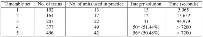
7.3 Computational results
We have tested some subsets extracted from the entire Southern Railway Decem-ber 2012 timetable, each corresponding to trains in real diagrams served by specific type(s). The original aim is to make comparisons with manual diagrams.