promoting access to White Rose research papers
White Rose Research Online [email protected]
Universities of Leeds, Sheffield and York
http://eprints.whiterose.ac.uk/
This is an author produced version of a paper published inRenewable Energy
White Rose Research Online URL for this paper:
http://eprints.whiterose.ac.uk/id/eprint/78161
Paper:
Millward-Hopkins, JT, Tomlin, AS, Ma, L, Ingham, DB and Pourkashanian, M (2013) Mapping the wind resource over UK cities.Renewable Energy, 55. 202 -211. ISSN 0960-1481
Mapping the Wind Resource over UK Cities
J. T. Millward-Hopkinsa,b, A. S. Tomlina*, L. Mab, D. B. Inghamb, M. PourkashanianbaEnergy Research Institute and thebEnergy Technology and Innovation Initiative (ETII), University of
Leeds, Leeds, UK, LS2 9JT
Abstract
Decentralised energy sources, such as small-scale wind energy, have a number of well-known advantages. However, within urban areas, the potential for energy generation from the wind is not currently fully utilised. One of the most significant reasons for this is that the complexity of air flows within the urban boundary layer makes accurate predictions of the wind resource difficult to achieve. Without sufficiently accurate methods of predicting this resource, there is a danger that wind turbines will either be installed at unsuitable locations or that many viable sites will be overlooked. In this paper, we compare the accuracy of three different analytical methodologies for predicting above roof mean wind speeds across a number of UK cities. The first is based upon a methodology developed by the UK Meteorological Office. We then implement two more complex methods which utilize maps of surface aerodynamic parameters derived from detailed building data. The predictions are compared with measured mean wind speeds from a wide variety of UK urban locations. The results show that the methodologies are generally more accurate when morecomplexity is used in the approach, particularly for the sites which are well exposed to the wind. The best agreement with measured data is achieved when the influence of wind direction is thoroughly considered and aerodynamic parameters are derived from detailed building data. However, some uncertainties in the building data add to the errors inherent within the methodologies.
Consequently, it is suggested that a detailed description of both the shapes and heights of the local building roofs is required to maximise the accuracy of wind speed predictions.
1 Introduction
Distributed energy sources in the form of micro-generation have a number of well know advantages: they reduce dependence upon energy imports, decrease transmission losses, and allow individuals to take more responsibility for their energy use. It has been suggested that potentially 40% of UK electricity could be sourced from micro-generation by the year 2050 [1], with small-scale wind energy contributing significantly to this. However, the industry is still in its infancy, particularly with regards to applications within urban areas.
A major barrier to the effective deployment of wind turbines in urban areas has been the lack of accurate methods for estimating wind speeds and energy yields at potential turbine sites. UK field trials carried out by the Energy Saving Trust [2] demonstrated this, showing substantial scatter in the relationship between measured wind speeds and those predicted by the Carbon Trust wind
estimator [3, 4]. To obtain an accurate resource assessment, ideally long-term measurements should be made on-site, at multiple heights [5]. However, for small-scale urban installations this is normally neither convenient nor financially viable. If sufficiently accurate methods of urban wind resource prediction were developed this may reduce the likelihood of customers purchasing turbines expecting unrealistically high energy yields, or companies installing turbines at unsuitable locations for ‘greenwashing’ purposes [6]. These unfavourable scenarios can be detrimental to the reputation of the wind energy industry as a whole.
It is possible to estimate mean wind speeds over an area analytically, as a function of height, by applying a ‘Wind Atlas Methodology’ [7]. This method requires information on both the regional wind climate and the roughness characteristics of the surface. The UK Met Office adopt this approach in their small-scale wind resource study [8], which was later developed into a freely available tool by the Carbon Trust [3]. The methodology involves scaling wind speeds from a regional wind climate up to a height at which the frictional effect of the surface is negligible, then scaling back down accounting for the effect of the surface roughness upon the wind profile. This is achieved using the standard logarithmic profile:
,
(1)
wherez0anddare the aerodynamic parameters of roughness length and displacement height,u*is
the friction velocity,κ is the Von Karman constant (≈ 0.4), and zis the height above the ground. Unfortunately, in urban areas it can be difficult to obtain accurate predictions using this type of methodology due to the difficulties in accurately estimatingz0anddfor urban surfaces [9] and the
influence of individual building aerodynamics upon the local wind resource [10]. However, new approaches for estimating wind profiles in urban areas [11-13] present an opportunity for improving the accuracy of these wind atlas methodologies.
In this paper, three different wind atlas methodologies for predicting above-roof mean wind speeds are tested in a number of UK cities. We use the Carbon Trust tool, then two more complex methods which utilize maps of aerodynamic parameters derived from detailed urban morphological
databases and consider wind directional effects [12]. To our knowledge, these latter models are the
0 *
ln
z d z u U
first to use detailed building databases, in conjunction with an advanced description of the effects of features such a building height heterogeneity [11-12], to map the wind resource over entire cities. After a discussion of the modelling approach and the input datasets, we use measured
meteorological data from a number of locations within each city to assess the accuracy of the methodologies. We then consider the source of model errors and how they may be reduced.
2 Wind Atlas Methodologies
2.1 The UK Met Office Approach
In this section the methodology developed by the UK Met Office [8] that underlies the Carbon Trust tool [3] is described, and is subsequently refered to as ‘model CT’ throughout this paper. The tool offers mean wind speed predictions at a location specified by its post code or grid reference and the potential turbine height. Unfortunately, at the time of writing the tool is no longer online. However, it is still valuable to compare its predictions with those of the more complex methodologies
developed in this paper as they indicate benchmark accuracy for a practical small-scale wind resource assessment method.
Fig. 1 (top) illustrates how the methodology predicts the mean wind speed for a given height. The first stage of the method involves taking a wind speed from a regional wind climate (UN) and scaling
this up to the top of the urban boundary layer (at heightzUBL) using the standard logarithmic wind
profile with a reference, ‘open country’ roughness length (z0-ref) of 0.14 m [8]. Therefore, the wind speed atzUBLis:
.
(2)
Here the regional wind climate is obtained from the NCIC database [8], which gives wind speeds over the whole of the UK, at a resolution of 1 km, which are valid at a height of 10 m above a smooth surface. The influence of any local topographical features of a horizontal length-scale greater than 1 km upon wind speeds are captured in this database. The UBL height,zUBL, is set to a constant value
of 200 m [8], and at this height the influence of the urban surface is assumed to be absent.
In the second stage of the methodUUBLis scaled down through the urban boundary layer (UBL) to
the blending height (zbl), where the flow is considered to be horizontally homogeneous [9]. Again, the logarithmic profile is used, and hence the wind speed atzblis:
.
(3)
Here, the aerodynamic parametersz0-fetchanddfetchare calculated on a regional scale by using ‘land
use data’ for the surrounding 1 km2in combination with a blending method [8,14]. This land use
data categorises the surface cover using classifications such as suburban, urban, and shrubland, at a
) 10 ln( ) ln( 0 0 ref ref UBL N UBL z z z U U
UBL fetch fetch
25 m resolution [8]. The Met Office estimate the blending height to be twice the maximum building canopy height in the same 1 km regional area.
Finally,Ublis scaled down to the turbine hub height (zhub) through the lowest region of the UBL. This
layer of flow is considered to be adapted to the local area in the surrounding 100-200 m, and hence aerodynamic parameters appropriate to the land cover in this area (z0-localanddlocal) are used to
estimate the wind speed atzhub:
.
(4)
Here, the values used forz0-localanddlocalare preselected by the UK Met Office for different ‘local
terrain types’, and the user is required to select the most appropriate terrain type for their site by using a number of visual aids and descriptions.
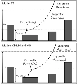
A complication with Equation (4) is that it is only valid down to the local mean building height, or the ‘canopy height’. Below this height, within the urban ‘canopy layer’, the flow is highly complex and spatially variable, and wind speeds will generally be too low for turbines to operate. However, as illustrated in Fig. 2 (top), an approximation of the canopy layer wind profile can be made using an exponential profile [15].
,
(5)
whereUhm-localis the wind speed athm-local, obtained using Equation (4), andλfis the fontal area
density of the local area (the ratio of the area of building faces to the total ground area). Here, the Carbon Trust tool assumes values forλfof 0.2 and 0.3 for suburban and urban local terrain types,
respectively.
2.2 Improving Estimates of Surface Aerodynamic Parameters
2.2.1 Estimating Roughness Length and Displacement Height using Detailed Building Data The second methodology we investigate (referred to as model CT-MH) uses the same process as model CT in order to correct a regional wind atlas for the effects of the surface roughness upon the wind profile. However the roughness lengths and displacement heights input into model CT-MH are estimated using a more detailed method.
For each of the cities investigated, maps of surface aerodynamic parameters are calculated using the method developed in Ref. [12]. The first stage of the method involves dividing each city into a grid of ‘neighbourhood regions’. Subsequently, the aerodynamic parameters of each region are estimated by inputting detailed building data for the city [16] into a morphological model [11,12]. These building data are available to the UK academic community and can be obtained online from
Landmap (http://www.landmap.ac.uk/) through the ‘Cities Revealed’ agreement (Cities Revealed © The GeoInformation Group 2008). Specifically, the data that is used in this work is from the ‘building
bl local local
local local hub bl hub z d z z d z U U 0 0 ln ln
9.6 1
exp f hub m-local local
-hm
hub U z h
heights’ feature collection, which includes information on the heights and footprints of manmade structures and woodland areas within the city, which were derived from LiDAR surveys and high resolution aerial photography.
We calculate maps of aerodynamic parameters for each of the cities on two different grids: a fine uniform grid (of 250 m resolution) and a coarse uniform grid (of 1 km resolution.) The resulting maps of aerodynamic parameters are used to representlocalandregionalscale aerodynamic parameters, respectively. This means that parameters from these 250 m resolution maps are used in Equation (4) forz0-localanddlocal,and parameters from the 1 km resolution maps are used in Equation (3) forz0-fetch
anddfetch.
For the current work, it is necessary to extend the method in Ref. [12] slightly as it is not appropriate for estimating the aerodynamic parameters of neighbourhoods with either very low or very high densities of buildings. This means it is necessary to estimate the aerodynamic parameters of these regions via other means in order to give a complete parameterisation of the cities aerodynamics. Consequently, for neighbourhoods with plan area densities (λp; defined as the ratio of total roof area
to total ground area in a neighbourhood region) within the range 0.03 to 0.75 we use the method in Ref. [12], while for the low or high density regions we assume the following values ofz0andd:
(i) when 0.01 <λp< 0.03, the neighbourhood is considered to be a ‘low density urban’ area, and
hence we assume:d/hm= 0.35 andz0/hm= 0.06, based on the recommendations in Ref. [9],
(ii) whenλp< 0.01, the number of buildings in the neighbourhood is assumed to be negligible, and
hence we assume aerodynamic parameters appropriate for open terrain:d= 0 andz0= 0.14 m [8],
(iii) when 0.75 <λp< 1, we assume the neighbourhood consists mostly of woodland, as built areas
very rarely become this densely packed, and hence we assign aerodynamic parameters:d/hm= 0.67
andz0= 1 m, based on the values in Refs. [8, 17].
There is of course a significant degree of uncertainty in these chosen values, and there are potentially other factors that could be considered to gain more accurate parameter estimates. However, this would require a detailed inspection of the neighbourhood regions on a case-by-case basis, which is impractical to carry out for multiple cities. Fortunately, the uncertainties in these assumptions are likely to have only a small influence upon the overall wind resource assessment, as for well over 90% of the neighbourhood regions in the cities studied here, 0.03 <λp< 0.75.
2.2.2 Other Modifications to the UK Met Office Methodology
There are a number of other aspects of model CT-MH that differentiate it from model CT. The first of these relates to the regional wind climate, for which the freely available NOABL database [18] is used in model CT-MH, rather than the NCIC database, due to reasons of availability. Secondly, the blending height is set to twice thelocalmean building height in model CT-MH, rather than the maximum height on a regional scale as in model CT. This is potentially a more appropriate blending height than that used in model CT, as the near surface flow over urban areas may adapt to the local underlying geometry over a relatively short distance, similar to the 250 m length-scale of the neighbourhood regions of the current work [10]. The two final differences, described below, are relevant only to wind speed predictions made close to, or below the top of the building canopy.
In the second stage of downscaling using model CT-MH the logarithmic profile of Equation (4) is only used down to the local ‘effective mean building height’ (hm-eff), rather than the local mean building
height as in model CT. This is illustrated in Fig. 2 (bottom). The heighthm-effis a modification of the
normal mean building height that accounts for the disproportionate effect of tall buildings upon the wind flow in areas where buildings are of heterogeneous height. It is predicted as part of the methodology used to estimatez0anddthat was described in the previous section [12]. Where
buildings are of heterogeneous heightshm-effindicates the height below which a logarithmic profile
can no longer describe the wind profile accurately.
Belowhm-effan exponential profile is used to describe the canopy layer wind profile, as in model CT.
However, a slight modification is made to Equation (5) to account for the influence of height variation upon the wind profile [19]:
.
(6)
Here,Uhm-eff-localis the wind speed athm-eff-localobtained from the log profile, andσhis the standard
deviation of the building heights in the local neighbourhood. Bothσhandλfare easily obtained
directly from the building data using the methodology detailed in Ref [12].
2.3 Incorporating the Influence of Changing Wind Direction
The most detailed method we implement (referred to as ‘model MH’) is the same as model CT-MH except for two significant modifications which are made to account for the influence of incoming wind direction upon the wind profile. An illustration of the model is shown in Fig. 1 (bottom).
Firstly, model MH accounts for the influence of incoming wind direction by describing the height of the UBL as a function of the distance from the upwind edge of the city (X; as illustrated in Fig. 1), rather than setting it to a constant as in models CT and CT-MH. This reflects the physical process of boundary layer growth, which occurs due to the fact that as the flow travels further into the city, vertical turbulent mixing leads to the frictional influence of the surface roughness extending
9.6 1 1
exp f m-local hub hm eff local local
eff hm
hub U h z h
upwards [8]. The estimation of this height is made using the formula of Elliot [20] for boundary layer growth, limited to a realistic, maximum height of 500 m [8, 21]:
.
(7)
Here,z0-refandz0-fetchare used for the ‘upwind’ and ‘downwind’ roughness lengths, respectively, and
the constant of 0.65 has been modified slightly from its original value of 0.75, as recommended by the Met Office [8]. It should be noted that determining the exact edge of a city, and henceX, can be quite subjective. However, the predicted wind speeds have a very low sensitivity toX, with the exception of those within a few hundred metres from the upwind city edge.
Secondly, model MH accounts for the influence of the incoming wind direction in the calculation of the aerodynamic parametersz0-fetchanddfetchthat are used in Equation (3). These parameters are
calculated by considering the aerodynamics of the upwind urban surface, rather than using regional (1 km scale) values as in models CT and CT-MH. The extent of the upwind area that is considered in the calculation is a 45° wide sector extending either to the cities edge or a maximum length of 5 km, as illustrated in Fig. 1 (bottom). The 5 km maximum sector length is chosen as Equation (7) suggests this is about the distance required for a fully developed UBL to develop (500 m deep) after a typical rural (z0 ≈ 0.14 m) to urban (z0 ≈ 1 m) surface cover change. Varying this maximum length between 4 km and 7 km had a negligible influence upon the results.
For each wind direction,z0-fetchis calculated from the values of roughness length lying within the
upwind sector by applying a blending method [22] to estimate the average, area-weighted frictional effect of the surface in that sector. The roughness lengths input into the blending method are derived from building data using the same method that was used for model CT-MH. However, they are now calculated for neighbourhood regions determined by anadaptivegrid rather than a uniform grid, as described in Ref. [MH12]. Unfortunately, there are no equivalent blending methods available to calculate an appropriate displacement height for use asdfetch. Therefore, for each wind direction,
dfetchis simply calculated as the arithmetic mean of the displacement height values from the adaptive
grid lying within the upwind sector. A summary of the differences in the input parameters used in each of the three models is given in Table 1.
3 Validation Datasets
3.1 Site Locations
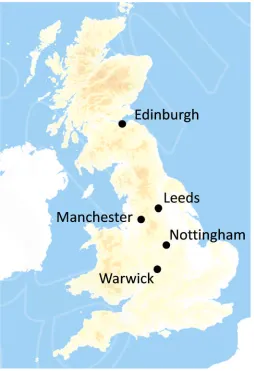
To evaluate the accuracy of the models described above we use measured wind speed data from a number of UK cities, namely Edinburgh, Leeds, Manchester, Nottingham, and Warwick/Leamington Spa. The locations of the cities range from the Midlands of England to the East coast of Scotland, as shown in Figure 3, and their sizes range from around 25 km2(Warwick) to over 500 km2
(Manchester). These cities were chosen partially as they span a broad range of UK city types but also due to the availability of appropriate meteorological data to evaluate the methodologies.
0.65 0.03ln , 500
The data used for the model evaluation were obtained from various measurement campaigns, including the Warwick Wind Trials [23] and several University and Met Office (MIDAS) weather stations [24-26]. Once these data were collated, mean wind speeds measured at 21 anemometers spread over the 5 cities were available to evaluate the models. Each site was at an independent geographical location, with the exception of those at Leeds University and Leeds City Council (two anemometers at different heights) and those at Eden, Southern and Aston Court (two anemometers at different locations).The sites cover a range of building types, from two-story suburban properties to medium-rise city-centre buildings and high-rise blocks of flats, and they lie within local areas that can broadly be categorised as residential, industrial, university campus or city centre. Basic
information on each of the sites is given in Table 2.
3.2 Measurement Details
The time period over which measurements were made at each site varied, as did the data coverage within each period. However, the measurement periods all lay within the five year period from 01/08/06 - 01/08/11. In order for each of the measured wind speeds (Umsr) to correspond to a
consistent time period each was extrapolated to be representative of this five year period (U5yr) by
using a simple correction factor accounting for the seasonal and annual variation in wind speed at a local reference site. For Edinburgh, Manchester and Nottingham, there were validation sites which had over 99% data coverage for the five year period, and hence these were appropriate to also be used as reference sites. For Leeds and Warwick, Met Office weather stations which were located a short distance outside each city and had continuous data coverage over the five years were chosen as reference sites. Further details on these reference sites are recorded in Table 2 alongside the information on the validation sites.
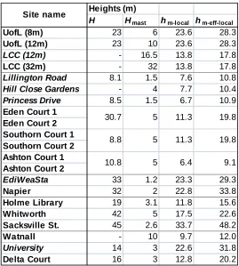
Details of the local geometry at each site are recorded in Table 3, including the anemometer mast height (Hmast), the building height (H), the local mean building height (hm-local), and the local effective
mean building height (hm-eff-local). These values ofH,hm-localandhm-eff-localwere calculated from the
same Landmap sourced building data that is used to derive the aerodynamic parameters. It can be seen that the effective mean building height is always greater than the mean building height.
For the majority of the validation sites the above ground measurement height (zhub) is simply taken
to be the sum of the anemometer mast height (Hmast) and the building height (H). For the remaining
sites, as the masts were not located on the highest part of the building roofs,zhubis set to be the sum
ofHand the height that the anemometer mast protrudes above the roof. Based upon the local geometrical details in Table 3, sites are then classified as ‘sheltered’ if the measurement height is lower than the local mean building height (zhub ‒ hm-local< 0) or if the measurement height is within 2
m of the buildings height (zhub ‒ H< 2). Any site not classified as sheltered is classified as ‘exposed’.
3.3 Implementing the Models
To test the accuracy of each of the three models, we make wind speed predictions at the above ground measurement height,zhub, for each of the validation sites in Table 2.
To obtain predictions using model CT it was necessary to specify the user inputs of ‘local terrain type’ and ‘canopy height’, in addition to the sites location and its above ground height. We chose the most appropriate local terrain type for each site from the available categories by using aerial
photography from Google Earth© to visually assess the local urban geometry. The local canopy height was then specified in two different ways: (i) using the default canopy height given by the tool for the particular local terrain type selected, and (ii) using the local mean building height (hm-local)
calculated from the Landmap building data. In the remainder of this paper we refer to these predictions as ‘CTdft’ and ‘CThm’, respectively.
In order to make predictions with models CT-MH and MH, we implement the methodologies using Matlab© to give mean wind speed predictions as a function of height for each city on a square, 250 m resolution grid. The mean wind speeds predicted for each validation site are easily obtained from these maps by determining which grid square each site lies within and then extracting the predicted wind speed at the corresponding measurement height.
4 Results and Discussion
4.1 Model Evaluation
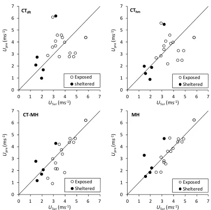
To evaluate the accuracy of each methodology, Fig. 4 shows scatter plots of the predicted (Upre) vs
measured (U5yr) wind speeds from all the validation sites. The figure suggests that the wind speed
predictions for these sites generally become more accurate when more complex methodologies are implemented. This is particularly evident for the exposed sites. To test this conclusion the mean percentage errors are calculated:
(8)
and the mean absolute error:
(9)
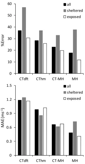
To calculate these errors the summations are made over all sites, and also for the exposed and sheltered sites separately, with the results summarised in Fig. 5. Two different metrics are
considered as each provides different sensitivities [4], and therefore it is useful to compare multiple metrics to test the robustness of the conclusions. For example, the %Error is more sensitive to errors at lower wind speed sites than the MAE.
yr yr pre
U
U
U
5 5
n
1
100
%Error
Upre U5yr
Fig. 5 confirms that the accuracy of the predictions increases with the level of detail included in the methodologies. The figure shows that for the chosen validation sites the predictions of the Carbon Trust Tool can be improved significantly (by about 8% and 0.2 ms-1in %Error and MAE, respectively)
by overriding the default canopy height with the local mean building height calculated from the building data. When model CT-MH is used there is a further reduction in overall errors of about 5% and 0.3 ms-1, which can be attributed to the more detailed manner in which surface aerodynamic
characteristics are calculated i.e. through the use of detailed building data as opposed to land use data. An additional reduction in errors of about 5% and 0.2 ms-1is achieved when model MH is used,
which highlights the advantages of thoroughly considering the influence of wind direction upon wind profiles in a prediction methodology. However, it is clear from Fig. 4 that even when using model MH the maximum and minimum errors are still significant.
Weekes and Tomlin [4] also considered the accuracy of the Carbon Trust tool in predicting mean wind speeds relevant to small-scale wind turbines. They also concluded that the accuracy of wind speed predictions can be increased significantly by considering a larger surrounding area in the calculation of aerodynamic parameters and accounting for the frequency of winds occurring from each direction.
It is important to also consider the variation in the performance of the models between the sheltered and exposed sites. It is evident from Fig. 5 that the methodologies generally perform better at the exposed sites, which is entirely as expected as the sheltered sites lie in complex regions of flow where wind speeds are influenced strongly by individual buildings. Local effects such as these are difficult to quantify without complex fluid dynamics (CFD) modelling, and hence the current methodologies are only expected to predict wind speeds at exposed sites with good accuracy. A useful observation is that if the accuracy of each methodology at just the exposed sites is
considered, then the enhanced performance of model MH is more pronounced. Specifically, for the exposed sites the %ERROR and MAE using model MH are 11.7% and 0.41 ms-1, respectively, while
the errors resulting from the use of model CTdftare 30.7% and 1.17 ms-1.
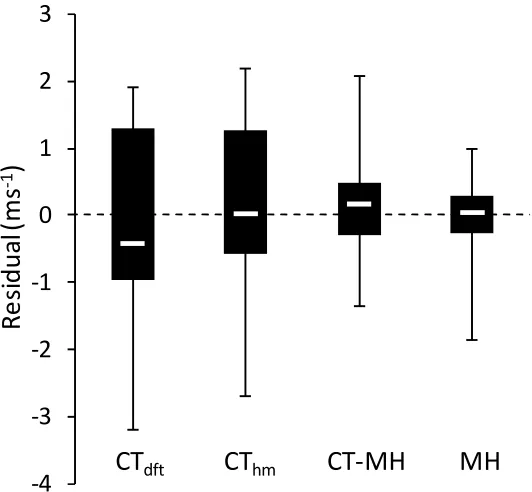
To determine if any bias exists in the predictions of each model, box plots are shown in Fig. 6 of the residual errors, defined asU5yr-Upre. These show that the predictions of models CThmand MH are
relatively unbiased, but model CTdfthas a tendency towards overestimations and CT-MH towards
underestimations. The bias in model CTdftis most likely due to the fact that the default local mean
building heights given by the tool are generally lower than those calculated from the building data. Consequently the local roughness length and displacement height used in the model can potentially be quite low compared to those used in the other methodologies. For model CT-MH the
underestimates are likely to occur because only a 1 km surrounding area is considered in the calculation ofz0-fetch. This means that in complex urban areas of high surface roughness, the values
calculated forz0-fetchcan be quite high relative to those that would be obtained if a larger, more
4.2 Sources of Model Errors
4.2.1 Uncertainties in the Modelling Approach
The previous section has shown that when using model MH it is possible to obtain reasonably accurate mean wind speed predictions for a variety of urban sites. However, significant errors could remain due to a number of uncertainties within the modelling approach. Firstly it has been
suggested that the NOABL database may slightly over-predict the wind climatology in urban areas [8]. The NCIC database may provide more accurate input data although it is unfortunately not freely available. In addition, the effect of local rooftop flow patterns upon the wind resource [10, 27] is not accounted for in such neighbourhood average approaches. Detailed CFD studies would be required in order to obtain detailed flow information around individual rooftops. It is expected however, that the MH model may provide useful boundary conditions for such studies. Uncertainties also occur when estimating aerodynamic parameters of real urban surfaces, even when using a relatively sophisticated morphological model such as that used in this work [11]. The Landmap building data that is used to derive the aerodynamic parameters also has a property which may amplify these errors and this will now be discussed in more detail.
4.2.2 Uncertainties in the Building Data
Within the Landmap building heights data set used in this work, each building is assigned only a single, above ground height. This means that assumptions have to be made for buildings with complex or pitched roofs and those located upon sloping ground. Consequently, the heights given in the data actually refer to thehighestpart of the roof above ground level, as noted in Ref. [12]. This can give rise to two issues: (i) it can significantly increase estimates of any ‘height parameters’ input into the model, such as mean building heights, effective mean building heights and displacement heights, and (ii) there can be discrepancies between the height of a building measured onsite and its height as obtained from the building data. In the current work, the latter issue has been minimised by taking the anemometer heights to be the mast height plus the building height contained in the building database. However, the former issue may explain some of the error in the model
predictions.
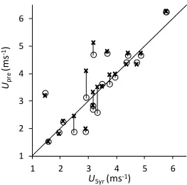
For this reason, in Fig. 7 we consider the effect of a small reduction in the three height parameters on the predicted wind speeds. This is done by recalculating the predictions for all the sites, using model MH, with the height parameters reduced by 10%. A value of 10% is chosen as the mean height a typical two story UK house with a 25° pitched roof [28] is about 90% of its maximum height. Clearly however, the difference between a buildings maximum and mean roof height will vary dramatically depending upon the building type, and hence this sensitivity test can offer only limited information on the potential for more detailed building data to improve the accuracy of model predictions.
Fig. 7 shows the new predicted wind speeds plotted alongside the original predictions for comparison. It is clear that the sensitivity of the predictions to the height parameters varies
improves only modestly: by about 1% and 0.03 ms-1in %Error and MAE, respectively at the exposed
sites.
Overall, this sensitivity test demonstrates that wind speed predictions near to the top of the building canopy are highly sensitive to the local canopy height. This implies that to maximise the accuracy of wind speed predictions it is crucial that height based inputs (i.e.hm,hm-effandd) are estimated as
accurately as possible, and additionally the heights of potential turbine installations must be estimated consistently with respect to morphological input data. In practice this may require a detailed description of the shapes of the local building roofs, in addition to their heights.
This sensitivity test indicates that using more detailed input building data may potentially improve the model predictions, and hence exploring how this can be achieved will be a focus of our future work.
5 Conclusions
Three different analytical methodologies for predicting mean wind speeds have been compared for various urban areas within the UK using measurements from 21 different sites, ranging from two-story suburban properties to medium-rise city-centre buildings and high-rise blocks of flats.
The methodologies generally became more accurate as more complexity was incorporated into the approach, particularly for sites which were not significantly sheltered by surrounding buildings, and were therefore well exposed to the wind. Significant improvements in accuracy were observed when aerodynamic parameters were derived from detailed building data, as opposed to land use data, and also when the influence of wind direction upon the wind profile was considered in detail. Both of these more detailed modelling approaches also led to a reduction in the bias of the predictions (when measured as the average residual error). Using the most detailed methodology at the well exposed sites, average percentage errors and mean absolute errors of 11.7% and 0.41 ms-1,
respectively, were achieved for mean wind speed predictions. The corresponding average residual error was small at 0.07 ms-1, indicating that the predictions were relatively unbiased with a very
weak tendency towards underestimating measurements. Considering the complexity of the
underlying urban surface, this is a reasonable level of accuracy for locations that could be considered as viable sites for the siting of small-scale turbines.
It is suggested that uncertainties within the building height data may contribute to prediction errors. This is particularly the case for sites which are near to the top of the building canopy, where
Acknowledgements The authors would like to thank The University of Edinburgh School of Geosciences, The University of Manchester Centre for Atmospheric Science, the UK Met Office, Leeds City Council, and all parties involved in the Warwick Wind Trials, for providing valuable field data used in this work, and Shemaiah Weekes (University of Leeds) for his insights. They would also like to thank the Engineering and Physical Sciences Research Council for providing the Doctoral Training Award which supported J. T. Millward-Hopkins during the research.
References
1. Microgeneration strategy (2006),www.berr.gov.uk/files/file27575.pdf, Department of Trade and Industry (30/8/12).
2. Location, location, location: Domestic small-scale wind field trial report (2009),
www.energysavingtrust.org.uk, Energy Savings Trust (30/08/12). 3. Wind Estimator,www.carbontrust.com(30/08/12).
4. S.M. Weekes, A.S. Tomlin, Evaluation of a semi-empirical model for predicting the wind energy resource relevant to small-scale wind turbines, Renewable Energy, 50 (2013) 280-288.
5. S.L. Walker, Building mounted wind turbines and their suitability for the urban scale—A review of methods of estimating urban wind resource, Energy and Buildings, 43 (2011) 1852-1862. 6. S. Stankovic, N. Campbell, A. Harries, Urban Wind Energy, Earthscan, London (p41) 2009.
7. L. Landberg, L. Myllerup, O. Rathmann, E.L. Petersen, B.H. Jørgensen, J. Badger, N.G. Mortensen, Wind Resource Estimation—An Overview, Wind Energy, 6 (2003) 261-271.
8. Small-scale wind energy Technical Report (2008), UK Met Office,
www.carbontrust.com/media/85174/small-scale-wind-energy-technical-report.pdf(30/08/12) 9. C.S.B. Grimmond, T.R. Oke, Aerodynamic properties of urban areas derived, from analysis of
surface form, Journal of Applied Meteorology, 38 (1999) 1262-1292.
10. J.T. Millward-Hopkins, A.S. Tomlin, L. Ma, D. Ingham, M. Pourkashanian, The predictability of above roof wind resource in the urban roughness sublayer, Wind Energy, (2011) 10.1002/we.463 11. J. Millward-Hopkins, A. Tomlin, L. Ma, D. Ingham, M. Pourkashanian, Estimating Aerodynamic
Parameters of Urban-Like Surfaces with Heterogeneous Building Heights, Boundary-Layer Meteorology, 141 (2011) 443-465.
12. J. Millward-Hopkins, A. Tomlin, L. Ma, D. Ingham, M. Pourkashanian, Aerodynamic Parameters of a UK City Derived from Morphological Data, Boundary-Layer Meteorology, 1-22.
13. S. Di Sabatino, E. Solazzo, P. Paradisi, R. Britter, A simple model for spatially-averaged wind profiles within and above an urban canopy, Boundary-Layer Meteorology, 127 (2008) 131-151. 14. P.J. Mason, The Formation of Areally-Averaged Roughness Lengths, Quarterly Journal of the
Royal Meteorological Society, 114 (1988) 399-420.
15. R.W. Macdonald, Modelling the mean velocity profile in the urban canopy layer, Boundary-Layer Meteorology, 97 (2000) 25-45.
16. Landmap: Spatial Discovery, Avaliable through the Cities Revealed agreement (Cities Revealed © The GeoInformation Group 2008),www.landmap.ac.uk(30/08/12).
17. J. Wieringa, Representative Roughness Parameters for Homogeneous Terrain, Boundary-Layer Meteorology, 63 (1993) 323-363.
19. D.H. Jiang, W.M. Jiang, H.N. Liu, J.N. Sun, Systematic influence of different building spacing, height and layout on mean wind and turbulent characteristics within and over urban building arrays, Wind and Structures, 11 (2008) 275-289.
20. W.P. Elliot, The Growth of the Atmospheric Internal Boundary Layer, Transactions of the American Geophysical Union, 39 (1958) 1048-1054.
21. R.E. Britter, S.R. Hanna, Flow and dispersion in urban areas, Annual Review of Fluid Mechanics, 35 (2003) 469-496.
22. E. Bou-Zeid, M.B. Parlange, C. Meneveau, On the parameterization of surface roughness at regional scales, Journal of the Atmospheric Sciences, 64 (2007) 216-227.
23. Encraft, Warwick Wind Trials Final Report,www.warwickwindtrials.org.uk (30/08/12). 24. School of GeoSciences Weather Station,www.geos.ed.ac.uk/abs/Weathercam/station
(30/08/12).
25. Whitworth Meteorological Observatory,
www.cas.manchester.ac.uk/restools/whitworth/index.html(30/08/12). 26. MIDAS Land Surface Stations data,www.badc.nerc.ac.uk(30/08/12).
27. S. Mertens, The energy yield of roof mounted wind turbines Wind Engineering, 27 (2003) 507-518.
Tables
Table 1: Summary of the input parameters used in each methodology
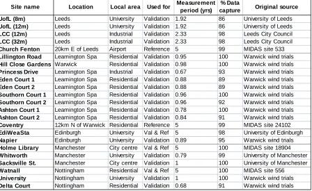
Table 2: Basic information on the measurement locations used as validation and/or a reference sites. UofL and LCC refer to the University of Leeds and the Leeds City Council, respectively.
Method
CT CT-MH MH
Pa ra m et er s
UN NCIC NOABL NOABL
z0-ref 0.14m 0.14m 0.14m
zUBL 200m 200m calculated from Eq. 7
dfetch and z0-fetch
from the 1km resolution aerodynamic parametermap
from the 1km resolution aerodynamicparameter map
calculated foreight different wind directions from the aerodynamic parameters lying within each sector
zbl twice the maximum canopy height in the 1km neighbourhood
2hm(from the 250m
resolution map) 2resolution map)hm(from the 250m
dlocal and z0-local
based upon local
terrain type from the 250m resolutionaerodynamicparameter map
from the 250m resolution aerodynamicparameter map
UofL (8m) Leeds University Validation 1.92 86 University of Leeds
UofL (12m) Leeds University Validation 1.92 86 University of Leeds
LCC (12m) Leeds Industrial Validation 2.33 98 Leeds City Council
LCC (32m) Leeds Industrial Validation 2.33 98 Leeds City Council
Church Fenton 20km E of Leeds Airport Reference 5 99 MIDAS site 533
Lillington Road Leamington Spa Residential Validation 0.95 100 Warwick wind trials
Hill Close Gardens Warwick Residential Validation 0.98 100 Warwick wind trials
Princess Drive Leamington Spa Industrial Validation 0.67 93 Warwick wind trials
Eden Court 1 Leamington Spa Residential Validation 0.88 89 Warwick wind trials
Eden Court 2 Leamington Spa Residential Validation 0.88 89 Warwick wind trials
Southorn Court 1 Leamington Spa Residential Validation 0.96 100 Warwick wind trials
Southorn Court 2 Leamington Spa Residential Validation 0.96 92 Warwick wind trials
Ashton Court 1 Leamington Spa Residential Validation 0.78 100 Warwick wind trials
Ashton Court 2 Leamington Spa Residential Validation 0.84 91 Warwick wind trials
Coventry 12km N of Warwick Residential Reference 5 99 MIDAS site 24102
EdiWeaSta Edinburgh University Val & Ref 5 98 University of Edinburgh
Napier Edinburgh University Validation 0.89 95 Warwick wind trials
Holme Library Manchester City centre Val & Ref 5 100 MIDAS site 18904
Whitworth Manchester University Validation 0.79 99 University of Manchester
Sacksville St. Manchester City centre Validation 1 100 University of Manchester
Watnall Nottingham Residential Val & Ref 5 100 MIDAS site 556
University Nottingham University Validation 1 100 Warwick wind trials
Delta Court Nottingham Residential Validation 0.68 91 Warwick wind trials
Location
Site name % Data
capture Original source Measurement
period (yrs) Used for
Table 3: Geometric characteristics at the validation sites. Sheltered sites are indicated by the italic text.
Heights (m)
H Hmast hm-local hm-eff-local
UofL (8m) 23 6 23.6 28.3
UofL (12m) 23 10 23.6 28.3
LCC (12m) - 16.5 13.8 17.8
LCC (32m) - 32 13.8 17.8
Lillington Road 8.1 1.5 7.6 10.8
Hill Close Gardens - 4 7.7 10.4
Princess Drive 8.5 1.5 6.7 10.9
Eden Court 1 Eden Court 2 Southorn Court 1 Southorn Court 2 Ashton Court 1 Ashton Court 2
EdiWeaSta 33 1.2 23.3 29.3
Napier 32 2 22.8 33.8
Holme Library 19 3.1 11.8 15.6
Whitworth 42 5 17.5 22.6
Sacksville St. 45 2.6 33.7 48.2
Watnall - 10 9.7 12.0
University 14 3 22.6 31.8
Delta Court 16 3 12.8 20.2
9.1 30.7
8.8
10.8 5
5
5 11.3 19.8
11.3 19.8
6.4
Figures
Figure 1: Schematic diagrams of each wind atlas methodology implemented in the current work
z0-ref
10m
UN
up-scale
dlocalandz0-local(250m)
dfetchandz0-fetch(1km)
200 m
UUBL
1stdown-scale
zbl Ubl
2nddown-scale
Urban boundary layer Internal boundary layer Model CT and CT-MH:
Uhub
Urban boundary layer Internal boundary layer
dlocalandz0-local(250m)
zUBL UUBL
1stdown-scale
zbl Ubl
2nddown-scale
Model MH (wind direction inclusive)
N NE
E
SE S SW W
NW
8 different wind directions considered using 5km maximum length, 45° wide sectors extending to the cities edge
z0-ref
10m
UN
up-scale
Uhub
dfetchandz0-fetch
distanceX
Figure 2: Illustration of the down-scaling process used by the methodologies to hub heights below the canopy top. Parameters controlling the profiles are given in brackets
hm-eff-local
Exp profile (λfandσ/hm)
Log profile (dlocal,z0-local)
Log profile (dfetch,z0-fetch)
Models CT-MH and MH
zbl
hm-local
Exp profile (λf)
Log profile (dlocal,z0-local)
Log profile (dfetch,z0-fetch)
Model CT
Figure 4: Comparisons of predicted (Upre) and measured, 5 year corrected (U5yr) wind speeds for each methodology 0 1 2 3 4 5 6 7
0 1 2 3 4 5 6 7
Upr
e
(m
s
-1)
U5yr(ms-1) CTdft Exposed sheltered 0 1 2 3 4 5 6 7
0 1 2 3 4 5 6 7
Upr
e
(m
s
-1)
U5yr(ms-1) CThm Exposed Sheltered 0 1 2 3 4 5 6 7
0 1 2 3 4 5 6 7
Upr
e
(m
s
-1)
U5yr(ms-1) CT-MH Exposed Sheltered 0 1 2 3 4 5 6 7
0 1 2 3 4 5 6 7
Upr
e
(m
s
-1)
U5yr(ms-1) MH
Figure 5: Average percentage errors (top) and mean absolute errors (bottom) calculated using each methodology over all the validation sites and also the sheltered and exposed sites separately.
0
10
20
30
40
50
60
CTdft
CThm
CT-MH
MH
%
Er
ro
r
all
sheltered
exposed
0
0.3
0.6
0.9
1.2
1.5
CTdft
CThm
CT-MH
MH
M
AE
(m
s
-1
)
all
Figure 6: Box plots of residual errors (ms-1) calculated over all the validation sites. These show the
inter-quartile range (black boxes), the median (white horizontal dashes) and the maximum and minimum errors (error bars).
-4
-3
-2
-1
0
1
2
3
Re
sid
ua
l(
m
s
-1
)
Figure 7: Sensitivity of the predictions of model MH to the ‘height parameters’. The original wind speed predictions (circles) and those with the height parameters reduced by 10% (crosses) are plotted against the measured, onsite wind speeds.
1
2
3
4
5
6
1
2
3
4
5
6
U
pre
(m
s
-1