This is a repository copy of
Feasible parallel-update distributed MPC for uncertain linear
systems sharing convex constraints
.
White Rose Research Online URL for this paper:
http://eprints.whiterose.ac.uk/90477/
Version: Accepted Version
Article:
Trodden, P. (2014) Feasible parallel-update distributed MPC for uncertain linear systems
sharing convex constraints. Systems & Control Letters, 74. pp. 98-107. ISSN 0167-6911
https://doi.org/10.1016/j.sysconle.2014.08.012
[email protected] https://eprints.whiterose.ac.uk/
Reuse
Unless indicated otherwise, fulltext items are protected by copyright with all rights reserved. The copyright exception in section 29 of the Copyright, Designs and Patents Act 1988 allows the making of a single copy solely for the purpose of non-commercial research or private study within the limits of fair dealing. The publisher or other rights-holder may allow further reproduction and re-use of this version - refer to the White Rose Research Online record for this item. Where records identify the publisher as the copyright holder, users can verify any specific terms of use on the publisher’s website.
Takedown
If you consider content in White Rose Research Online to be in breach of UK law, please notify us by
Feasible parallel-update distributed MPC for uncertain linear systems sharing convex
constraints
IPaul Trodden∗
Department of Automatic Control&Systems Engineering University of Sheffield, Sheffield S1 3JD, UK
Abstract
A distributed MPC approach for linear uncertain systems sharing convex constraints is presented. The systems, which are dynamically decoupled but share constraints on state and/or inputs, optimize once, in parallel, at each time step and exchange plans with neighbours thereafter. Coupled constraint satisfaction is guaranteed, despite the simultaneous decision making, by extra constraint tightening in each local problem. Necessary and sufficient conditions are given on the margins for coupled constraint satisfaction, and a simple on-line scheme for selecting margins is proposed that satisfies the conditions. Robust feasibility and stability of the overall system are guaranteed by use of the tube MPC concept in conjunction with the extra coupled constraint tightening.
Keywords: control of constrained systems; predictive control; decentralization; time-invariant
1. Introduction
Providing optimal control and decision-making to a system is very desirable. For such purposes, model predictive control (MPC) [1] has achieved more widespread adoption and greater impact in industry than any other modern control technology; for example, MPC has largely replaced traditional PID loops as the controller of choice in the process control industry [2]. The popularity of MPC is not restricted to industry, and significant advances have been made by academic researchers on theoretical properties such as stability and robustness [3].
When the system to be controlled is large in scale, or phys-ically or organizationally disjoint, centralized MPC may be impractical or undesirable for reasons of computation, communi-cation and the single point of failure. Completely decentralized MPC, on the other hand, in which subsystem controllers make decisions independently and without coordination, can result in poor performance and even instability [4]. Thus, attention
has focused ondistributedMPC [5], wherein controllers share
information. The challenge is then how should computation and communication be used to coordinate actions and achieve system-wide feasibility, stability and optimality.
Many approaches to distributed MPC have now been pro-posed, and comprehensive surveys are given in [6, 7]. Algo-rithms are broadly divisible according to the classes of system to which they apply [5]: for instance, linear versus nonlin-ear dynamics; coupling via the dynamics versus coupled via constraints. The focus of this paper is on systems comprising multiple, dynamically-decoupled subsystems, each with linear
IThis paper was not presented at any IFAC meeting. ∗Tel.+44-114-222-5679. Fax+44-114-222-5683.
Email address:[email protected](Paul Trodden)
time-invariant dynamics. The subsystems, which are subject to bounded, persistent disturbances, are coupled via shared con-straints on states and/or inputs. The presence of such concon-straints has been identified as a key open research problem for DMPC [2]. One of the main difficulties is in determining the set of condi-tions under which coupled constraint satisfaction is ensured despite the decision-making of independent controllers. Algo-rithms are either hierarchical or distributed (i.e., with or without a supervisory, coordinating agent), iterative or non-iterative, and sequential or parallel in the timing of updates [5].
Iterative distributed approaches include those based on pri-mal decomposition, in which controllers share information, and bargain or coordinate with local neighbours [8–10]; dual de-composition approaches where iteration is to primal feasibility (satisfaction of coupled constraints) [11–13]; and, a coopera-tive scheme wherein distributed control agents augment their decision spaces to include the inputs subject to shared con-straints [14].
con-troller to maintain the state within the tube for any realization of the disturbance. Similar to [15], constraint tightening is used to guarantee feasibility in the presence of uncertainty; however, the sequence dependency and the need for all subsystems to optimize at each time step is removed, leading to a scheme with low and flexible levels of communication [17]. Both approaches, however, have limitations imposed by their sequential/serial na-ture: [15] requires sufficient time within a sampling interval for the entire sequence of optimization problems to be solved. On the other hand, [17] permits only one (or, strictly, non-coupled) subsystems to optimize at each time step, which can lead to poor performance.
The feasible parallel-update DMPC proposed in this paper avoids these limitations by permitting thesimultaneous optimiz-ing of subsystems’ plans at each time step while maintainoptimiz-ing robust feasibility and stability. The advantage of low and flex-ible communication is retained, since no inter-agent iteration
or negotiation is required, andanynumber of subsystems may
optimize at a time step. The approach is a significant extension of [15, 17], in that the reliance on sequential or serial updat-ing is removed. Subsystems maintain satisfaction of convex coupled constraints on states and/or inputs, despite optimizing simultaneously, by tightening their local representations of the coupled constraints. Comparable approaches include the tube-based schemes recently proposed by Farina and Scattolini [19] and Riverso and Ferrari-Trecate [20] for dynamically-coupled, deterministic subsystems sharing constraints. These also achieve coupled constraint satisfaction despite parallel updating: in the former, predicted state and input trajectories are constrained to lie within time-invariant neighbourhoods around known-feasible references, and coupled constraints are tightened accordingly. In the latter, the tube MPC concept is applied twice, leading to a double tightening of constraints. Other approaches include those iterative methods that maintain primal feasibility across iterates [9, 14, 21] and, therefore, can be terminated after a sin-gle iteration. However, in none of these papers is an explicit mechanism given for selecting the margins by which coupled constraints are tightened. A key contribution of this paper is that a simple and explicit scheme is proposed for the on-line calcu-lation of margins by which to tighten coupled constraints. The margins are time-varying, both with sampling time and along the prediction horizon, and are calculated from information transmit-ted between controllers at the previous time step. Necessary and sufficient conditions are given on the size of margins for robust coupled constraint satisfaction. Moreover, robust feasibility and stability of the closed-loop system is established for any number of subsystems optimizing simultaneously at each time step.
The paper is organized as follows. The problem is stated in Section 2. This is followed by a review of single-update tube DMPC [17] in Section 3. In Section 4, the necessary and suffi-cient margins for simultaneous coupled constraint satisfaction are developed, followed by the presentation of the proposed feasible parallel-update DMPC in Section 5. The approach is demonstrated by numerical examples in Section 6. Finally, Sec-tion 7 concludes the paper.
Notation and conventions:. The non-negative and positive reals (integers) are denoted, respectively,R0+andR+(N0+andN+).
Givena,b ∈N0+, withb >a,N[a,b] ,{a,a+1, . . . ,b−1,b}.
NbdenotesN[0,b]. The cardinality of a finite setAisn(A). For
xi ∈ Rn,i ∈ N[a,b], withb > a, (xi)i∈N[a,b] means (xa,xa+1, . . . ,
xb−1,xb)∈ R(b−a)n. x(−i) means (x1, . . . ,xi−1,xi+1, . . . ,xn). For
a,b∈Rn,a≤bapplies element by element. ForX,Y ⊂Rn, the Minkowski sum isX⊕Y ,{x+y: x∈ X,y∈Y}; forY ⊂X, the Pontryagin difference isX⊖Y,{x∈Rn :Y+x⊂X}. For
X⊂Rnanda∈Rn,X⊕ameansX⊕ {a}.AXdenotes the image of a setX ⊂Rnunder the linear mappingA:Rn7→Rp, and is given by{Ax: x ∈ X}. A polyhedron is the intersection of a finite number of halfspaces, which is convex, and a polytope is a closed and bounded polyhedron, and is also convex. ForX⊂Rn,
the support function ish(X,y),sup{y⊤x:x∈X}fory∈Rn. A
setX⊂Rnis positively invariant (PI) for a systemx+= f(x) if and only if for allx∈Xit holds that f(x)∈X. A setX⊂Rnis robust positively invariant (RPI) for a systemx+= f(x,w) if and
only if for allx∈Xand allw∈Wit holds thatf(x,w)∈X. The notationx(k+j|k) indicates a prediction ofxfor jsteps ahead fromk.
2. Problem statement
2.1. System dynamics
Consider a set of dynamically decoupled subsystems,I=
{1, . . . ,Ni}. A subsystem i ∈ Ihas the linear time-invariant, discrete-time dynamics
x+i =Aixi+Biui+wi, (1)
where xi ∈ Rni,ui ∈ Rmi,wi ∈ Rni are, respectively, its state, control input and disturbance. x+
i is the successor state. The existence of a stabilizing control law Ki for each (Ai,Bi) is assured by the following assumption.
Assumption 1. For eachi∈ I, Ai,Biis stabilizable, and the statexiis known exactly by the controller foriat each sampling instant.
2.2. Local constraints
The state and input of each subsystemi∈ Iare subject to local constraints
xi∈Xi, ui∈Ui,
while the disturbancewiis unknowna prioribut lies in a setWi.
Assumption 2. For eachi∈ I,Xiis closed and convex,Uiis
compact and convex, and each contains the origin in its interior.
Wi⊂Xiis compact and convex, and contains the origin (but not
2.3. Shared constraints
Coupling between subsystems exists in the form of a set of shared constraints, C = {1, . . . ,Nc}. A shared constraint
c∈ Cinvolves a subset of subsystems,Ic⊆ I, and acts on the collection ofcoupling outputsof those subsystems as follows.
zc,(zci)i∈Ic ∈Zcwherezci=Ecixi+Fciui,∀i∈ Ic. (2)
Here,zci∈Rrciandzc∈Rrc whererc=Pi∈Icrci. This is a
gen-eral form of coupling constraint: a constraintcpermits coupling between the states and/or inputs of any subset of subsystems.
Assumption 3. For eachc∈ C,Zcis a closed, convex
polyhe-dron, containing the origin in its interior.
It follows thatZcmay be represented byMclinear inequalities:
Zc=Zc(qc),{z∈Rrc :p⊤
cmz≤qcm,∀m∈N[1,Mc]} (3)
wherepcm ∈Rrc,qcm∈R+, for allm∈N[1,Mc]. The matrix and
vector that collectpcmandqcm, respectively, arePc∈RMc×rcand
qc=(qc1,qc2, . . . ,qcMc)∈R
Mc
+ , so that (3) may also be written
asZc={z∈Rrc :P
cz≤qc}.
2.4. Coupling structure
The following definitions identify structure in the coupling between subsystems, and are used to determine what informa-tion a local subsystem controller needs. By construcinforma-tion,Ic=
i ∈ I
: (Eci,Fci) ,0, and the subset of constraints in which subsystemi ∈ Iis involved isCi =c ∈ C : (Eci,Fci) ,0. Then, the set of other subsystems sharing constraints with a subsystemiisQi=Sc∈CiIc
\ {i}.
2.5. Control objective
The control objective is to regulate the state of each subsys-tem to the origin while satisfying all constraints and minimizing the infinite-horizon, system-wide cost function
∞ X
k=0
X
i∈I
li xi(k),ui(k), (4)
whereli:Rni×mi 7→R0+,li(xi,ui)≥kk(xi,ui)kfor somek>0
andli(0,0)=0.
3. Overview of single-update tube MPC
The single-update tube DMPC approach [17] is based on the “tube MPC” concept [18], wherein the controller designs a sequence of disturbance-invariant state sets for the system to follow. The sets are centered on the nominal trajectory; that is, the state predictions obtained by applying the optimized con-trol sequence to the disturbance-free dynamics. In a distributed setting, each subsystem controller designs a tube for its local subsystem to follow. Use of a local feedback controllerKi along-side the implicit MPC control law then guarantees that each subsystem state remains within its tube, despite the action of the disturbancewi, and without the need to re-optimize at every
time step (as is done in conventional MPC and DMPC). There-fore, by permitting only a single subsystem to optimize at each time step, and subsequently communicating to other subsys-tems information about its new tube, robust coupled constraint satisfaction, feasibility and stability are guaranteed [17]. The re-mainder of this section more formally describes, and introduces key assumptions and definitions used later in the paper.
3.1. Distributed optimal control problem
With subsystemiat a statexi(k) at timek, the distributed optimal control problem (DOCP-i) is
Ji0 xi(k),z∗i(k)=min
ui(k) n
Ji ui(k):ui(k)∈ Ui xi(k),z∗i(k)
o
. (5)
The vectorz∗
i(k) denotes coupling output information from other subsystems needed byito solve its problem at timek, and is described later; it is included as an index to the optimal cost
J0
i and feasible setUito highlight the dependency of each on
the coupling outputs of other subsystems, and the coupling be-tween DOCPs. The decision variableui(k) contains the initial state prediction, ¯xi(k|k), and the sequence of future controls,
¯
ui(k|k),u¯i(k+1|k), . . . ,u¯i(k+N−1|k). The cost function is a finite-horizon approximation to the infinite-horizon, local cost in (4):
Jiui(k),Fi x¯i(k+N|k)+ N−1
X
j=0
li x¯i(k+j|k),u¯i(k+j|k),
where Fi:Rni 7→ R0+. The feasible setUi xi(k),z∗i(k)is de-fined by the following constraints for all j∈NN−1.
xi(k)−x¯i(k|k)∈ Ri, (6a)
¯
xi(k+ j+1|k)=Aix¯i(k+j|k)+Biu¯i(k+j|k), (6b)
¯
xi(k+ j|k)∈Xi⊖ Ri, (6c)
¯
ui(k+j|k)∈Ui⊖ Si, (6d)
¯
xi(k+N|k)∈ Xfi, (6e)
¯
zci(k+j|k)=Ecix¯i(k+j|k)+Fciu¯i(k+j|k),∀c∈ Ci, (6f)
¯
zci(k+j|k),z¯∗c(−i)(k+j)∈Zc⊖ Tc,∀c∈ Ci. (6g)
The details of this feasible set are now described. Ri in (6a)
is an RPI set for the uncertain subsystem i under the local
feedback law ui = Kixi, i.e., for the closed-loop dynamics
x+i = (Ai+BiKi)xi+wi. Note the existence ofRi is assured by Assumptions 1 and 2. In this paper, we assume the following.
Assumption 4. For eachi∈ I,Riis a polytope with 0∈ Ri.
Note that this assumption is not restrictive, and tools and meth-ods are available for computing polytopic invariant sets—or ap-proximations to them—and corresponding control laws, e.g. [22–
24]. To minimize conservativeness, it is desirable thatRi be
chosen as small as possible [18].
Ui,Zcand, respectively, setsRi,Si,KiRi,Tc,Qi∈IcEciRi⊕ FciSi, forc∈ Ci. (Note that, by Assumption 4 and linearity,Si andTcare polytopic and contain the origin [25]). The following assumption limits the size of these tightening sets, and is mild for most applications.
Assumption 5. For eachi ∈ I,Ri ⊂ Xi,Si ⊂ UiandTc ⊂
Zc,∀c∈ C.
The terminal setXf
iin (6e) is a PI set for the nominal subsys-tem dynamics under the local terminal control lawui =κif(xi),
i.e., for the closed-loop dynamicsx+i =Aixi+Biκfi(xi).
Assumption 6. For eachi ∈ I,Xf
i is a polytope with 0∈ X
f i, and Xf
i ⊆ Xi ⊖ Ri, κfi(X f
i) ⊆ Ui⊖KiRi, and Qi∈Ic EciX
f
i ⊕
Fciκfi(Xf i)
⊆Z
c⊖ Tcforc∈ Ci.
The terminal set is used in conjunction with the terminal costFi, under the following assumption. Note that Assumptions 6 and 7 are common, and correspond to A1–A4 in [3].
Assumption 7. For eachi ∈ I,Fi Aixi+Biκfi(xi)−Fi(xi) ≤ −li xi, κfi(xi),∀xi∈ Xfi.
Finally, as previously mentioned, the feasible setUidepends not only on the sampled local state xi(k) but also on the cou-pling outputs of subsystems sharing constraints withi. In (6g), ¯
z∗c(−i)(k+ j) denotes the collection of coupling outputs at pre-diction step jfrom subsystems sharing constraintc∈ Ciwith subsystemi,i.e., the collection of ¯z∗
cq(k+ j) overq∈ Pc. (Alter-natively viewed, the minus subscript notation means all elements of ¯z∗
c(·) excluding ¯z∗ci(·).) Thenz
∗
i(k) is defined as the collection of ¯z∗
c(−i)(k+j) over allj∈NN−1andc∈ Ci. How this informa-tion is obtained is described later. First, the tube DMPC control law and algorithm are outlined.
3.2. The tube DMPC control law and single-update algorithm
With subsystem i at state xi(k) at time k, assume that a
feasible (but not necessarily optimal) solution to DOCP-i is
available,i.e.,
u∗i(k),x¯∗i(k|k),u¯∗i(k|k),u¯∗i(k+1|k), . . . ,u¯∗i(k+N−1|k).
Then the control applied to a subsystemiis
u∗i(k)=u¯∗i(k|k)+Ki xi(k)−x¯∗i(k|k)
.
(7)
By construction, all constraints are satisfied at timek: xi(k)∈ ¯
x∗i(k|k)⊕ Ri⊂Xi,u∗i(k)∈u¯∗i(k|k)⊕ Si⊂Uiandz∗c(k)∈z¯
∗
c⊕ Tc⊂
Zc. Subsequently, using the control (7), the state of subsystemi
evolves asx∗i(k+1)∈Aix¯∗i(k|k)+Biu¯∗i(k|k)⊕(Ai+BiKi)Ri⊕Wi= ¯
x∗i(k+1|k)⊕(Ai+BiKi)Ri⊕Wi⊆x¯∗i(k+1|k)⊕ Ri, and, since ¯
x∗i(k+1|k)⊕ Ri⊂Xiand ¯u∗i(k+1|k)⊕ Si⊂Ui, local state and input constraints remain satisfied at timek+1, regardless of disturbances. Moreover,z∗
c(k+1)∈z¯∗c(k+1|k)⊕ Tc⊂Zc, so coupled constraints are also satisfied. Therefore, it is simple to show that a feasible solution to each DOCP-ican be constructed without solvinganyoptimization problem at timek+1:
˜
ui(k+1),x¯∗i(k+1|k),u¯∗i(k+1|k), . . . ,
¯
u∗i(k+N−1|k), κfi( ¯x
∗
i(k+N|k)). (8)
Moreover, no information exchange is needed to construct these
solutions at timek+1. This suggests the following scheme,
used in [17]: a single subsystem, sayi, (or, strictly, a set of subsystems not sharing any constraints) optimizes at timek+1, solving its DOCP-ito obtain a solutionu0
i(k+1) (not necessarily equal to ˜ui(k+1)) givenxi(k+1) and the coupling information z∗i(k+1), which is constructed fromz∗(k). All other subsystems renew existing feasible plans from timekvia (8). The optimizing
subsystemicommunicates its new plan to coupled subsystems
q ∈ Qi. At timek, therefore, the coupling informationz∗i(k) needed byiis the collection of ¯z∗cq(k+j|kˆq) over all j∈NN−1,q∈ Pc,c ∈ Ci, where ˆkq is the time at which subsystem q last updated by optimization.
When the system is controlled according to this algorithm, robust coupled constraint satisfaction, feasibility and stability of the closed-loop system is guaranteed [17].
3.3. Centralized optimal control problem
For later use, we define the corresponding centralized opti-mal control problem (COCP). For the system at a statex(k)=
xi(k)i∈Iat timek:
J0 x(k)=min
u(k)
( X
i∈I
Ji ui(k):u(k)∈ U x(k)
)
(9)
whereu(k), ui(k)i∈I, and the feasible setU x(k)is defined by (6a)–(6f) for alli∈ Iand the coupling constraint
¯
zc(k+j|k)∈Zc⊖ Tc,∀c∈ C,j∈NN−1.
The next result, which is adapted from Theorem 3.1 in [17], follows from construction of the constraint sets, and states that each and every subsystemihas a feasible solution to its DOCP-i
if and only if the collection of these individual solutions is a feasible solution to the COCP.
Lemma 1. u∗i(k)i∈I ∈ U x(k)
⇐⇒ u∗
i(k)∈ Ui xi(k),z
∗
i(k)
,
for all i ∈ I, where, for each i ∈ I,z∗i(k)is the collection of
¯
z∗cq(k+j)(obtained fromu∗q(k)) over all j∈NN−1,q∈ Ic,c∈ Ci.
4. A tightening procedure for parallel coupled constraint satisfaction
The key to the robust coupled constraint satisfaction of [17] is the single-update restriction. With the system at a state
xi(k)i∈I, and, supposing a feasible solutionu∗i(k) exists to each DOCP-i, it is clear that the coupled constraints are satisfied, since (6g) holds for eachi, with ¯z∗
ci(k),¯z
∗
c(−i)(k)
∈Z
c⊖ Tc. If, then, a single subsystemi∈ Ioptimizes for someu0
i(k),u
∗
(k), then (6g) ensures coupled constraint satisfaction is maintained.
However, if two subsystemspandqthat share some constraint
cwere to optimize simultaneously, then coupled constraint sat-isfaction is not guaranteed. This is because although solving
DOCP-pand DOCP-qindependently, obtainingu0
p(k) andu0 q(k) respectively, will satisfy the individual constraints
¯
in DOCP-p, where ¯z∗c(−(p,q))(·),¯z∗ci(·) i∈Ic\{p,q}
, and
¯
z0cq(k+j|k),z¯∗cp(k+j),z¯∗c(−(p,q))(k+ j)∈Zc⊖ Tc
in DOCP-q, at all steps j∈NN−1, it will not necessarily lead to
satisfaction of
¯
z0cp(k+j|k),¯z0cq(k+j|k),¯z∗c(−(p,q))(k+j)∈Zc⊖ Tc.
In this paper, the single-update restriction is lifted, and any
number of subsystems, a subsetIopt ⊆ I, is permitted to
op-timize simultaneously at a time step. The development that permits this is the systematic tightening of (6g) in the distributed optimal control problem, restricting the feasible region for i
so that two or more coupled subsystems can optimize simul-taneously. The modified DOCP is defined in the next section; subsequently, a systematic procedure for determining the modi-fied coupled constraint is developed.
4.1. Modified coupled constraint and distributed optimal control problem
The modified distributed optimal control problem
(MDOCP-i) for subsystemiat statexi(k) is
˜
Ji0 xi(k),z∗i(k)=min
ui(k) n
Jiui(k):ui(k)∈U˜i xi(k),z∗i(k)
o
(10)
where ˜Ui(xi,z∗
i) is defined by (6a)–(6f) and the constraint
¯
zci(k+j|k),¯z∗c(−i)(k+j)∈Z˜ci(j). (11)
The set ˜Zci(j) replaces the setZc⊖ Tcin the problem, and is permitted to vary over the horizon. We require the following assumption.
Assumption 8. For eachi ∈ I,c∈ Ciand j ∈ NN−1, the set
˜
Zci(j)⊆Zc⊖ Tcis a closed polyhedron.
To construct ˜Zci(j), we use the same Mcnormal vectors that define, in (3), the original coupled constraint setZc, but a
different right-hand side:
˜
Zci(j),Zc q˜ci(j)={z∈Rrc :P
cz≤q˜ci(j)}, (12)
where ˜qci(j)∈RMc. Then specification of ˜Zci(j) is reduced to the
problem of specifying ˜qci(j), and this is our aim in this Section. We derive the following conditions on ˜qci(j): first, a lower bound to guarantee at all times the existence of feasible solution to each subsystem’s MDOCP; second, an upper bound that ensures the collection of solutions, across optimizing subsystems, satisfies all coupled constraints.
In what follows, to make clear the dependence of the feasible set for problem MDOCP-ion ˜qci(j), we write ˜Ui xi(k),z∗i(k),
˜
qi(k)), where ˜qi(k) is the collection of ˜qci(j) overc∈ Ci and
j∈NN−1for subsystemi. The following lemma, which holds
because the only difference between to DOCP-iand MDOCP-i
is tighter coupling constraints in the latter, will be useful in later results.
Lemma 2. Given xi(k) and z∗
i(k) = z¯
∗
c(−i)(k+ j)
c∈Ci,j∈NN−1
such thatUi xi(k),z∗i(k)is non-empty,U˜i xi(k),z∗i(k),qi(˜ k)⊆ Ui xi(k),z∗i(k).
4.2. Lower bound onq˜ci(j) to ensure existence of a feasible solution to MDOCP-i
The consequence of Lemma 2 is that a solution to MDOCP-i
is also a feasible solution to DOCP-i. The result in this subsec-tion establishes condisubsec-tions under which the opposite statement is true: given a solution to DOCP-i, it is also a feasible solution to MDOCP-i. In particular, a lower bound on ˜qci(j) is given, so that the modified coupled constraint set (12) is not tightened so much that an existing feasible solution is excluded.
Proposition 1. Suppose that, for a subsystem i∈ Iwith state xi(k)at time k, there exists au∗i(k)∈ Ui xi(k),z∗i(k), wherez∗i(k)
is the collection ofz¯∗cq(k+ j)over all j∈NN−1,q∈ Ic,c∈ Ci.
Thenu∗i(k)∈Ui˜ xi(k),z∗i(k),qi(˜ k)if and only if
˜
qci(j)≥Pc¯z∗c(k+j), (13)
for all j∈NN−1,c∈ Ci, wherez¯∗c(k+j)= z¯∗cr(k+j)r∈Ic.
Proof. The solutionu∗
i(k) ∈ Ui xi(k),z
∗
i(k)
satisfies all con-straints (6) by construction, and henceu∗i(k) satisfies (6a)–(6f) in MDOCP-i. Therefore, to prove thatu∗i(k)∈U˜i xi(k),z∗i(k),qi(˜ k) it is necessary and sufficient to show thatu∗i(k) satisfies the re-maining constraint in MDOCP-i, (11).
The coupling constraints (6g) in DOCP-i, satisfied by con-struction, have
¯
z∗ci(k+j|k),z¯∗c(−i)(k+j)
=z¯∗c(k+j)∈Zc(qc)⊖ Tc
for all j∈NN−1,c∈ Ci. Satisfaction of (6g) by the same ¯z∗c(·) means ¯z∗
c(k+ j)∈ Z˜ci(j) for j∈ NN−1,c∈ Ci. Rewriting this condition in terms of support functions,
¯
z∗c(k+j)∈Z˜ci(j) ⇐⇒ v⊤z¯∗c(k+j)≤hZ˜ci(j),v,∀v∈Rrc,
and j∈NN−1,c∈ C. Given the polyhedral description of ˜Zci(j) in (12) asZcq˜ci(j), it is necessary and sufficient to evaluate these support function inequalities atv= pcm,m=1. . .Mc, thus
hZc q˜ci(j),pcm
≥p⊤cmz¯∗c(k+j),m=1. . .Mc.
Finally, by definition of the support function,hZc q˜ci(j),pcm
≤ ˜
qci(j), and so ˜qci(j)≥Pc¯z∗c(k).
4.3. Upper bound onq˜ci(j)to ensure system-wide coupled con-straint satisfaction
Now we consider the situation where a subset of subsystems, sayIopt(k), solve their MDOCPs simultaneously at timek, while all remaining subsystems continue to follow plans from a previ-ous time step (renewed via (8)). Given that a constraintc∈ C involves the setIc⊆ Iof subsystems (a total numbern(Ic)), Iopt
(k) contains some subsetIoptc (k),Iopt
(k)∩ Icof the sub-systems sharing constraintc, a total numbernIoptc (k)≤n(Ic). A necessary condition for maintaining feasibility of the overall system is
¯
zci(k+j|k)i∈Ioptc (k) | {z }
optimizing
, ¯z∗cr(k+j)r∈Ic\Ioptc (k) | {z }
non-optimizing
∈Zc(qc)⊖ Tc,
That is, the coupling outputs of all the optimizing subsystems, when taken together and with those of non-optimizing subsys-tems, must satisfy the coupling constraints.
The result in this subsection establishes conditions under which satisfaction of (14) is guaranteed for any choice ofIopt(k). In particular, an upper bound on ˜qci(j) in (12) is developed, which limits the maximum size of the coupled constraint set in
each MDOCP-i. Alternatively viewed, the result corresponds
to a minimum amount by which the original coupled constraint set must be tightened in order to guarantee coupled constraint
satisfaction when the MDOCP-iproblems are solved
simultane-ously.
Proposition 2. Suppose that, for each subsystem i∈ Iwith state xi(k)at time k, there exists au∗i(k)∈ Ui xi(k),z∗i(k), wherez∗i(k)
is the collection of¯z∗cq(k+j)over all j∈NN−1,q∈ Ic,c∈ Ci.
Further suppose thatu0
i(k)∈ Ui˜ xi(k),z
∗
i(k),qi(˜ k)
, for all i∈
Iopt(k)⊆ I. Then
¯
z0ci(k+j|k)i∈Ioptc (k), ¯z ∗
cr(k+j)r∈Ic\Ioptc (k)
∈Zc(qc)⊖ Tc, (15)
for all j∈NN−1, c∈ C, if
X
i∈Ioptc (k)
˜
qci(j)≤qc−tc+(N opt c −1)Pc¯z
∗
c(k+j), (16)
where tc=h(Tc,pc1),h(Tc,pc2), . . . ,h(Tc,pcMc) ⊤
.
Proof. Consideru0
i(k)∈U˜i xi(k),z
∗
i(k),qi˜
fori∈ Iopt
(k). This satisfies (6a)–(6f) and (11) by construction. In particular, con-straint (11) has
¯
z0ci(k+j|k),¯z∗c(−i)(k+j)∈Zc q˜ci(j)
for all j∈NN−1,c∈ Ci. Summing both sides of this constraint, via Minkowski addition, over alli∈ Ioptc (k),
X
i∈Iopt
c (k)
¯
z0ci(k+j|k),z¯c∗(−i)(k+j)∈ M
i∈Iopt
c (k)
Zc q˜ci(j).
Expanding the summation and noting that ¯z∗c(k+j)= z¯∗ci(k+
j)i∈Ic,
¯
z0ci(k+j|k)i∈Iopt
c (k), z¯ ∗
cr(k+j)
r∈Ic\Ioptc (k)
+ n Ioptc (k)−1z¯∗c(k+j)∈
M
i∈Ioptc (k)
Zcq˜ci(j).
Written in terms of support functions,
v⊤z¯0ci(k+j|k)i∈Ioptc (k), z¯ ∗
cr(k+j)
r∈Ic\Ioptc (k)
≤ −n Ioptc (k)−1v⊤z¯∗c(k+j)+
X
i∈Ioptc (k)
hZc q˜ci(j),v,
for all j∈NN−1,c∈ Candv∈ Rnc. Likewise, writing (15) in
terms of support functions,
v⊤z¯0ci(k+j|k)i∈Ioptc (k), z¯
∗
cr(k+j)
r∈Ic\Ioptc (k)
≤h Zc(qc),v−h Tc,v,
for j∈NN−1,c∈ Candv∈Rnc. It is necessary and sufficient
to evaluate these support function inequalities atv=pcm,m= 1. . .Mc. Comparing these expressions, it follows that (15) is satisfied if
− n Ioptc (k)−1p⊤cm¯z∗c(k+j)+
X
i∈Ioptc (k)
hZcq˜ci(j),pcm
≤hZc(qc),pcm−hTc,pcm.
for m = 1. . .Mc,c ∈ C,j ∈ NN−1. Therefore, noting that
h Zc(qc),pcm=qcmandh
Zcq˜ci(j),pcm
≤q˜cim(j),
X
i∈Ioptc (k)
˜
qci(j)≤qc−tc+(N opt
c −1)Pc¯z∗c(k+j),
wheretc,h(Tc,pc1),h(Tc,pc2), . . . ,h(Tc,pcMc) ⊤
.
Remark 1. The bounds (13) and (16) have interpretations in terms of the slackness of the coupled constraints. Themth com-ponent ofqc−tc−Pc¯z∗c(k+ j) is equal to the slack remaining in constraintc, at prediction stepj, in the directionpcm, given the known coupling outputs ¯z∗
cr(k+j) of eachr∈ Ic. Rewriting (16),
X
i∈Ioptc (k) ˜
qci(j)−Pc¯z∗c(k+j)≤qc−tc−Pc¯z∗c(k+j),
which states that the total space allowed to simultaneously opti-mizing subsystems sharing constraintc, in directionpcm, should not exceed the slack remaining in that direction. The lower bound (13) ensures that the solutionu∗
i(k) remains a feasible choice for each optimizing subsystemi ∈ Iopt(k), by not per-mitting the feasible region to shrink so much that this point is excluded. Note that if no slack remains in directionpcmof con-straintc, then ˜qcim(j)=qcm−tcm: no tightening is permitted in that direction.
4.4. Main result
The main result of this Section draws together the previous results, establishing conditions under which solving MDOCPs in parallel leads to guaranteed system-wide feasibility.
Theorem 1. Suppose that, for each subsystem i∈ Iwith state xi(k)at time k, there exists au∗i(k) ∈ Ui xi(k),z∗i(k), where
z∗i(k) is the collection of z¯∗cq(k+ j) over all j ∈ NN−1,q ∈ Ic,c ∈ Ci. Then, for all i ∈ Iopt and any Iopt ⊆ I, if qi˜
satisfies(13)and(16), (i)U˜i xi(k),z∗i(k),qi˜ is non-empty and
containsu∗i(k); (ii) for anyuis(k)∈U˜i xi(k),z∗i(k),qi˜, the
col-lection ofus
i(k)i∈Iopt(k) together withu∗r(k)r<Iopt(k) satisfy all
local and coupling constraints:
uis(k)i∈Iopt(k), u
∗
r(k)
r<Iopt(k)
∈ U x
(k).
Proof. (i) Existence follows from Proposition 1: for alli ∈
Iopt(k), and anyIopt(k)⊆ I, if ˜qci(j)≥Pc¯z∗
c(k+j),∀c∈ Ci,j∈
NN−1 in the MDOCP-i, then there exists a feasible solution, namelyu0
i(k) =u
∗
The implication is thatanysubset of subsystems may opti-mize simultaneously, and (i) a feasible solution to each problem is guaranteed to exist, (ii) all coupled constraints remain satis-fied, if the coupled constraint set in subsystemsi’s MDOCP is chosen asZc q˜ci(j), with ˜qci(j) satisfying (13) and (16). Theo-rem 1 assumes the existence and availability of such ˜qci(j), but the question remains of whether such ˜qci(j) can be found easily. The upper bound (16) in particular is a coupled constraint, and therefore implies some coordination is required to determine individual ˜qci(j) for eachi∈ Ioptc (k). The following result con-firms that suitable ˜qci(j) always exist, and suggests a simple scheme for choosing them.
Proposition 3. For i∈ Iopt(k)⊆ I, the choice
˜
qci(j)= qc−tc+(βci−1)Pc¯z
∗
c(k+j)
βci , (17)
for j ∈ NN−1, c ∈ Ci, satisfies(13) and (16) for all βci ≥
n Ioptc (k)≥1andz¯c∗(k+j)∈Zc(qc)− Tc.
Proof. Suppose that ¯z∗c(k+j)∈Zc(qc)− Tc,∀j∈NN−1,c∈ C
at timek, and consider some subset of subsystemsIopt(k)⊆ I so that Nopt(k) ≥ 1. By construction, n Iopt
c (k) ≥ 1 for all
c∈Si∈Iopt(k)Ci. Fori∈ Iopt(k), let ˜qci(j) be given by (17), with
someβci ≥n I
opt
c (k), for all j∈NN−1,c∈ Ci. Then, because ¯
z∗c(k+j)∈Zc(qc)− TciffPc¯z∗c(k+j)≤qc−tc,
˜
qci(j)=qc−tc+(βci−1)Pc¯z
∗
c(k+j) βci
≥Pcz¯
∗
c(k+j)+(βci−1)Pc¯z
∗
c(k+j)
βci =Pc¯z
∗
c(k+j)
hence satisfaction of (13). To show (16), for eachc∈Si∈Iopt(k)Ci,
sum (17) overIoptc :
X
i∈Ioptc (k) ˜
qci(j)= X
i∈Ioptc (k)
qc−tc+(βci−1)Pc¯z∗c(k+j) βci
= X
i∈Ioptc (k)
qc−tc βci +
X
i∈Ioptc (k)
(βci−1)Pc¯z∗c(k+j)
βci .
Becauseβci≥nI opt
c (k)≥1,∀c,i, thenPi∈Ioptc (k) qc−tc
βci ≤qc−tc.
Likewise,Pi∈Ioptc (k)
(βci−1)Pc¯z∗c(k+j)
βci ≤
n Ioptc (k)−1
PC¯z∗c(k+ j)
for allβci≥n I opt
c (k)≥1. Hence (16) is satisfied.
Here a largerβcicorresponds to more tightening of the cou-pling constraint set in MDOCP-i: asβci → ∞then ˜qci(j) →
Pc¯z∗
c(k+j),i.e.,Zcq˜ci(j)→ z¯∗c(k+ j). In practice, it is de-sirable to have ˜qci(j) as close as possible to the original size of the constraint set, after tightening for robustness to disturbances,
i.e., (qc−tc). This suggests smallβci; however,βciis lower-bounded asβci≥nIoptc (k), where the latter is the number of optimizing subsystems sharing constraintc, implying a practi-cal lower limit on the amount of tightening required to ensure robustness to simultaneous decision making. Note that if the op-timizing set,Iopt
(k), is selected so thatnotwo subsystems within it are coupled, thenn Ioptc (k)=1 for allcand ˜qci(k)=qc−tcif
βciis chosen equal to 1: then MDOCP-ibecomes identical to the DOCP-i. For any other choice ofIopt(k), so thatnIopt
c (k)≥2 for somec, optimizing subsystems share the slack remaining in the constraint evenly.
5. Feasible parallel-update distributed MPC
In this section, the main distributed MPC algorithm is pre-sented, including a distributed algorithm for the initialization step, with guaranteed convergence to a feasible solution. Finally, robust feasibility and stability results are established.
5.1. Feasible parallel-update distributed MPC algorithm
The revised DOCP, with on-line computation of ˜qci(j), is used in the following algorithm.
Algorithm 1 (Feasible parallel-update DMPC for subsystemi).
Offline:ComputeKiandκif, setsRi,Si,Tc,X f
i. Tighten lo-cal constraint setsXi,Uiand determine the vector,tc, of support functions toTc.
Online:
1. Setk=0. Obtain an initial feasible solution using Algo-rithm 2.
2. Sample current statexi(k). 3. Update plan:
Ifi∈ Iopt(k)
(a) Extract ¯z∗c(k+j),∀c∈ Ci,j∈NN−1,fromz∗i(k).
(b) Set ˜qci(j)= qc−tc+(βci−1)Pcz¯
∗
c(k+j)
βci ,∀c∈ Ci,
j∈NN−1, withβci≥nIoptc (k). (c) Obtainu0
i(k) as solution to MDOCP-i. (d) Transmit coupling information ¯z0
ci(k+j|k),j∈NN−1, to coupledq∈ Qi.
(e) Setu∗i(k)=u0i(k).
Elserenew current plan via (8):u∗
i(k)=u˜i(k). 4. Buildz∗
i(k+1), via (18), using new information received from coupled updating subsystemsq∈ Qi∩ Iopt(k) and previous information from coupled non-updating subsys-temsr∈ Qi\ Iopt(k).
5. Applyui(k)=u¯∗i(k|k)+Ki xi(k)−x¯∗i(k|k). Wait one time step, incrementk, go to step 2.
Details of Algorithm 1 are now described. The algorithm begins with the off-line computation of feedback laws and con-straint sets. Following this, Algorithm 2, which will be described in Section 5.2, is employed at the initialk=0 step. At a subse-quent time stepk, a subset of subsystems,Iopt(k), the choice of which is unrestricted, optimize plans by solving their respective MDOCPs. Subsystems not inIopt(k) renew their current plans via (8). The on-line calculation of ˜qci(j) for use in the MDOCP-i
assumed that each subsystem knows how many other coupled subsystems will optimize at timek, this assumption may be too strong and inflexible in some cases. Instead, it is sufficient to setβci=n(Ic)—where this is the total number of subsystems sharing constraintc—and sincen(Ic) ≥ nIoptc (k)by defini-tion, then this allows all subsystems to optimize in parallel, at any time step, without the need for further communication or
a-prioriarrangement. Though such an approach may add un-necessary tightening, hence conservatism, in many applications sparsity exists in the coupling constraints (a constraintcdoes not couple all subsystems) andn(Ic) may be significantly smaller than the number of subsystems.
Following optimization, subsystemsi∈ Iopt
exchange infor-mation with coupled neighbours, as per step 3d. The received information is used, in step 4, to build the coupling information z∗
i(k+1) for use at the next time step,k+1. For subsystemi considering the coupling output of subsystemr, this is done as
¯
z∗cr(k+ j)=
¯
z0
cr(k+ j|k), r=i ¯
z0cr(k+ j|k), r∈ Qi∩ Iopt(k), ¯
z0
cr(k+ j|kˆr), r∈ Qi\ Iopt(k),
(18)
for j ∈ N[1:N], where ˆkr is the last time at which subsystemr
solved its MDOCP.
5.2. A distributed algorithm for initialization
The following algorithm is employed as the initialization step of Algorithm 1. For clarity of notation, we denote the original coupled constraint setZc(qc)⊖ Tc,i.e., that in (6g), as
¯
Zc.
Algorithm 2 (Initialization for a subsystemi).
1. For allc∈ Ci, obtain ¯Zi
cas the projection of set ¯Zconto the subspaceRrci.
2. Measurexi(0), setp=0, and obtainu[ip]as solution to
min
ui Ji(ui)
subject to (6a)–(6f), ¯zci(j)∈Z¯ic,∀j∈NN−1,c∈ Ci. (19)
3. Transmit coupling information ¯z[cip](j),j ∈ NN−1 to
cou-pled subsystemsq∈ Qi.
4. If(6g) is satisfied by ¯z[cip](j) together with ¯zc[(p−]i)(j),∀j ∈
NN−1,c∈ Ci, terminate. Else
(a) Obtainu[ip+]as solution to
Di
u[ip+],u[−pi]=min
ui
N−1
X
j=0
X
c∈Ci
1
n(Ic)d
¯
zci(j),z¯[c(p−]i)(j),Z¯c
subject to (6a)–(6f) (20)
(b) Setu[ip+1]=wiu [p+]
i +(1−wi)u [p]
i , wherewi>0 and
P
i∈Iwi=1.
(c) Incrementpand go to step 3.
In this algorithm, subsystems begin by decoupling the cou-pled constraint sets, via a projection onto the subspace corre-sponding to the local subsystem’s coupling outputs. Conse-quently, the subsystems obtain initial solutions satisfying local constraints, but not necessarily coupled constraints. To work towards coupled constraint satisfaction, the subsystems follow the iterative procedure of steps 3 and 4. The following result, the proof of which may be found in Appendix A, establishes convergence to an initial feasible solution satisfying all coupled constraints.
Proposition 4. (Convergence of Algorithm 2) Suppose that
U x(0),∅and letu[ip] be the sequence generated, for each i∈ I, by Algorithm 2. Then, for all i∈ I, (i) problem(19)is feasible; (ii) problem(20)is feasible at every iteration p; (iii) the cost function Du[p], where
D(u), N−1
X
j=0
X
c∈C
dz¯c(j),Z¯c
andu = u1, . . . ,uNi
, is non-increasing with iteration p; (iv) the cost sequencenDu[p]oconverges to
0and the solutions
{up}converge to the feasible setU(x(0)).
Remark 2. The optimality of obtained solutions, and hence closed-loop performance of the proposed DMPC, with respect to the system-wide objective and tube-based CMPC, will depend on (i) the optimality of the solutions obtained at initialization, and (ii) the size and description of the coupled constraint sets following the on-line extra tightening. The former is influenced by the weightswi,i∈ I, and has been well studied in the litera-ture. The latter depends on theβciparameter used in (17), and is a topic of current research.
5.3. Robust feasibility and stability
The remainder of this section shows that system-wide robust feasibility and stability are guaranteed for any update sequence {Iopt(k)}.
Theorem 2(Robust feasibility and stability). Suppose that, for each i ∈ I,u∗i(k)exists and is a feasible (but not necessarily optimal) solution to DOCP-i at time k. Consider some optimiz-ing set of subsystems,Iopt(k)⊆ I. Then, (i)u∗
i(k)is a feasible
solution to MDOCP-i for i∈ Iopt(k); (ii) any feasible (but not
necessarily optimal) solution,u0
i(k), to problem MDOCP-i for
each i∈ Iopt(k)satisfies
u0i(k)i∈Iopt, u
∗
r(k)
r<Iopt
∈ U(x(k)) ;
(iii) for all xi(k+1)∈Aixi(k)+Biui(k)⊕Wi, where
ui(k)=
¯
u0i(k|k)+Ki xi(k)−x¯0i(k|k) i∈ Iopt(k) ¯
u∗
i(k|k)+Ki xi(k)−x¯∗i(k|k)
i<Iopt(k), (21)
the candidate solutionui(˜ k+1)is a feasible solution to DOCP-i for all i∈ I, and MDOCP-i for all i∈ Iopt
(k+1)⊆ I; (iv) each cost function is monotonically decreasing:
Jiu∗i(k+1)
≤J
i u∗i(k)
−l
i x¯∗i(k|k),u¯
∗
i(k|k)
whereu∗
i(k+1)is the solution adopted by i at time k+1.
Sub-sequently, (v) the closed-loop system controlled by Algorithm 1 is robustly feasible and xi(k)→ Riand ui(k)→KiRias k→ ∞,
for each i∈ I, for any choice of update sequenceIopt(k) k≥0.
Proof. Parts (i) and (ii) follow directly from Theorem 1. For part
(iii), sinceu∗i(k)∈ Ui xi(k),z∗i(k),∀i,then u∗i(k)i∈I ∈ U x(k)
(Lemma 1). From [17], it follows that
˜
ui(k+1)∈ Ui xi(k+1),z∗i(k+1),∀i∈ I, ˜
ui(k+1)i∈I ∈ U x(k+1) .
and from Theorem 1 that ˜ui(k+1)∈Ui˜ xi(k+1),z∗i(k+1),qi(˜ k+ 1),∀i∈ Iopt(k+1)⊆ I. For (iv), givenu∗
i(k), with cost
Ji u∗i(k)
=F
i x¯∗i(k+N|k)
+
N−1
X
j=0
li x¯∗i(k+j|k),u¯
∗
i(k+j|k)
the solution ˜ui(k+1) is a feasible solution atk+1, with cost
Jiui(˜ k+1)=Fi
Aix¯∗i(k+N|k)+Biκ f i x¯
∗
i(k+N|k)
+li
¯
xi∗(k+N|k), κfi x¯∗i(k+N|k)
+ N−1
X
j=1
li x¯∗i(k+j|k),u¯
∗
i(k+j|k)
≤Ji u∗i(k)
,
where the inequality follows from Assumption 7. Furthermore, an optimizing subsystemi∈ Iopt
(k+1) at stepk+1 obtains a solutionu0i(k+1), with costJiu0i(k+1)≤Jiui(˜ k+1). All
r<Iopt
adopt ˜u(k+1), costJr ur(˜ k+1). Thus,Ji u∗i(k+1)≤
Ji ui(˜ k+1), whereu∗i(k+1) is the adopted solution.
Part (v) follows by recursion: an initial feasible collection u∗
i(0) ∈ Ui xi(0),z∗i(0)
implies all subsequent optimizations are feasible, and u∗
i(k)
i∈I ∈ U x(k)
regardless of update sequence Iopt(k)
k≥0. Convergence of each xi(k) to Ri and
ui(k)→KiRifollows from the monotonicity ofJand the stan-dard arguments [3].
6. Numerical example
Consider four identical point masses with
Ai=
"
1 1
0 1
#
, Bi=
"
0.5 1
#
,
and local constraint setsXi = xi ∈ R2 : −[10,5]⊤ ≤ xi ≤
[10,5]⊤ ,Ui = ui ∈ R : −1 ≤ ui ≤ 1. A single coupled
constraint restricts the local control inputs across all subsystems to a value less than the sum of the local limits:
zi=
h
0 0ixi+1ui,
4
X
i=1
|zi| ≤2.5
The local objectives areli xi,ui = x⊤i Qixi+u⊤i Riui, with Qi,
[image:10.595.307.563.100.166.2]Ri to be defined, and a zero terminal cost. The disturbance
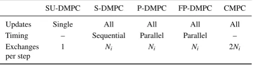
Table 1: Comparison of DMPC schemes.
SU-DMPC S-DMPC P-DMPC FP-DMPC CMPC
Updates Single All All All All Timing – Sequential Parallel Parallel – Exchanges
per step
1 Ni Ni Ni 2Ni
set isWi = wi ∈ R2 : kwik∞ ≤ 0.05. For simplicity, the
local controller is nilpotent,i.e., Ki =−[1 1.5], the terminal law isκfi =Ki, and together withXf
i ={0}, robust asymptotic convergence toRi = Wi⊕(Ai +BiKi)Wi is assured. Initial conditions arexi =5,−2
⊤
,∀i, and the prediction horizon is
N=8.
Five different control schemes are used:
1. ‘SU-DMPC’: single-update DMPC [17], wherein a single, different subsystem optimizes per time step;
2. ‘S-DMPC’: sequential DMPC, similar to [15], wherein all optimizewithina time step, in a sequence. Feasibility is guaranteed by each subsystem sharing its new plan before the next-in-line subsystem updates;
3. ‘P-DMPC’: parallel DMPC, wherein all optimize in paral-lel, but with no extra tightening of coupled constraints; 4. ‘FP-DMPC’: the proposed feasible-parallel DMPC; 5. ‘CMPC’: centralized MPC.
To allow direct comparisons, each of the distributed controllers is initialized using Algorithm 2, even though the published SU-DMPC and S-SU-DMPC schemes, [17] and [15] respectively, as-sume a centralized initialization. Note that for each scheme, a subsystem shares its new plan immediately after updating. Owing to the different updating arrangements (parallel versus sequential; single versus all), this leads to different levels of communication, as shown in Table 1.
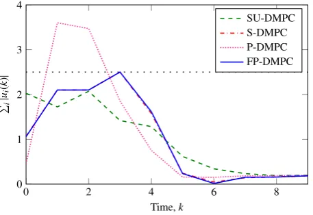
Figure 1 shows, forQi =I,Ri =1, the total control effort used at each time step. The in-parallel optimizations of P-DMPC lead to a sustained constraint violation. All other schemes satisfy the coupled constraint, and FP-DMPC can be seen to use the full range. Note that although S-DMPC and FP-DMPC are apparently similar, there is more variation in the individualui for the former, which is not perceptable in the figure.
Table 2 shows the closed-loop costs obtained for each con-troller. Two scenarios are shown: scenario 1, with identical cost matricesQi = I,Ri = 1, and scenario 2, with differing costs,