Testing Implications of the Adaptive Market Hypothesis via Computational Intelligence

(1)

This is a repository copy of

Testing Implications of the Adaptive Market Hypothesis via

Computational Intelligence

.

White Rose Research Online URL for this paper:

http://eprints.whiterose.ac.uk/76733/

Version: Accepted Version

Proceedings Paper:

Kazakov, Dimitar Lubomirov orcid.org/0000-0002-0637-8106 and Butler, Matthew Richard

(2012) Testing Implications of the Adaptive Market Hypothesis via Computational

Intelligence. In: Computational Intelligence for Financial Engineering & Economics (CIFEr),

2012 IEEE Conference on. 2012 IEEE Computational Intelligence for Financial

Engineering and Economics (CIFEr 2012), 29-30 Mar 2012 IEEE , USA , pp. 1-8.

https://doi.org/10.1109/CIFEr.2012.6327799

[email protected] https://eprints.whiterose.ac.uk/ Reuse

Items deposited in White Rose Research Online are protected by copyright, with all rights reserved unless indicated otherwise. They may be downloaded and/or printed for private study, or other acts as permitted by national copyright laws. The publisher or other rights holders may allow further reproduction and re-use of the full text version. This is indicated by the licence information on the White Rose Research Online record for the item.

Takedown

If you consider content in White Rose Research Online to be in breach of UK law, please notify us by

(2)

Testing Implications of the Adaptive Market Hypothesis via

Computational Intelligence

Matthew Butler and Dimitar Kazakov

Abstract—This study analyzes two implications of the Adaptive Market Hypothesis: variable efficiency and cyclical profitability. These implications are, inter alia, in conflict with the Efficient Market Hypothesis. Variable efficiency has been a popular topic amongst econometric researchers, where a variety of studies have shown that variable efficiency does exist in financial markets based on the metrics utilized. To determine if non-linear de-pendence increases the accuracy of supervised trading models a GARCH process is simulated and using a sliding window ap-proach the series is tested for non-linear dependence. The results clearly demonstrate that during sub-periods where non-linear dependence is detected the algorithms experience a statistically significant increase in classification accuracy. As for the cyclical profitability of trading rules, the assumption that effectiveness waxes and wanes with the current market environment, is tested using a popular technical indicator, Bollinger Bands (BB), that are converted from static to dynamic using particle swarm optimization (PSO). For a given time period the parameters of the BB are fitted to optimize profitability and then tested in several out-of-sample time periods. The results indicate that on average a particular optimized BB is profitable, active and able to outperform the market index up to 35% of the time. These results clearly indicate the cyclical nature of the effectiveness of a particular trading model and that a technical indicator derived from historical prices can be profitable outside of its training period.

I. INTRODUCTION

The Adaptive Market Hypothesis (AMH) of Lo [14][15] offers an alternative market theory to Fama’s Efficient Mar-ket Hypothesis (EMH) [5] that has several conflicting as-sumptions. These include the issues of bounded rationality of individual investors, path dependence of the equity-risk premium and variable market efficiency. The last assumption, that of variable efficiency, has been a popular topic amongst econometric researchers, where a variety of studies have shown that it does exist [2] [13] [20] in the financial markets for the metrics considered. These studies have also revealed that market efficiency is not a convergence but is in fact cyclical. This evidence supports the AMH and implies that a non-zero probability exists for creating trading strategies that outperform the market. Given that markets appear to exhibit non-linear correlations there still remains the question whether or not active trading strategies or technical analysis can take advantage of these inefficient market periods. The observation that market efficiency is cyclical is dependent on the robustness of the statistical test. From a forecasting point of

Matthew Butler and Dimitar Kazakov are with the Artificial Intelli-gence Group in the Department of Computer Science, The University of York, Deramore Lane, Heslington, York, UK (email: {mbutler, kaza-kov}@cs.york.ac.uk).

view the most important question, assuming a cyclical nature to market efficiency, is whether or not these periods of non-linear dependence can be used to improve forecasting accuracy and therefore lead to more profitable trading models. The previous work on market efficiency was mainly concerned with demonstrating that efficiency was episodic and that a relationship existed between the maturity of the market and its degree of market efficiency. The results from each of the studies [20] [13] revealed that emerging markets tended to be less efficient than mature markets. In 2009, Todea et al. [18] analyzed if the profitability of an optimal moving average (MA) strategy was contingent on the market period. The results were obtained for six Asia-Pacific financial markets and in five of the markets the MA strategy was more profitable in periods that exhibited non-linear dependencies. These results however do not reflect any out-of-sample testing as an optimal strategy was determined a priori for a particular market and the results do not reveal if any advantages exist for forecasting future price trends. This is the motivation behind this research, to determine if the presence of non-linear dependencies in a time series offers any benefits to forecasting models devel-oped from machine learning techniques. The word presence is emphasized as the actual data generating process is not known and any dependencies identified are contingent on the robustness of the statistical test.

(3)

experimental results moot. This conclusion, of course, is based on the fact that an active technical trading rule that cannot outperform the passive buy and hold approach is irrelevant and is evidence against the AMH. Alternatively, we could use an active learning approach where an optimal trading strategy can be constructed for the majority of market environments. This approach would ensure that each trading model tested was at one time profitable and able to outperform the passive buy-and-hold approach. In section III-A we discuss the exact methodology used for choosing BBs fitted using PSO and how the results are evaluated.

II. VARIABLEEFFICIENCY

To analyze the effect of non-linear dependence in a time-series, on the forecasting accuracy of Supervised Learning, a generalized autoregressive conditional heteroskedasticity (GARCH) model is used to simulate a financial time-series. A GARCH model, as the name suggests, allows for conditional variance that is not constant through time (a characteristic that is commonly observed in financial time series). The form of a GARCH(1,1) process for a series of discrete observations {Yt} is given below:

Yt = σtǫt (1)

σ2

t = α0+α1Y_t2

−1+β1σ

2

t−1 (2)

where ǫt is standard Gaussian white noise and the condition that α1+β1 < 1. Equations 1 and 2 return a white noise process with non-constant conditional variance, where the variance depends on the previous return. Equation 2 can be easily extended to include more lags. For the purpose of this study a GARCH(2,2) model was chosen. In the next section the methodology for identifying episodic non-linear dependence is explained.

A. Non-linear Dependence

The methodology for this study is based on [13] [2] where a sliding window approach is used to partition the time series into subsamples that exhibit random walk behaviour and non-linear dependence. For a time series {Yt}T1 and a window of size d an initial sub-sample is created consisting of observations {Yt}d1, the appropriate tests are run and then the window shifts by one day to cover {Yt}d+12 and so forth until the end of the sample {Yt}TT−d. The window size used

in this study is the same as [18] which is 200 observations. Within each sliding window the sample is tested for non-linear dependence using the Hinich Portmanteau bi-correlation (H) test [6]. Prior to applying the Portmanteau tests the data within the sliding window undergoes two stages of pre-processing. First, the series {Yt}T1 is considered to be a non-stationary stochastic process and to aid with the analysis the series is transformed to stationary by converting the series to continuously compounded percentage returns, as follows:

rt=log(yt/yt−1)∗100 (3)

wherertis the daily percentage return for timet. The second step is to standardize the data within each window to have a

sample mean of zero and a sample standard deviation of one, as follows:

Z(t) = R(t)−mR

σR

(4)

where Z(t) is the standardized series,mR is the sample mean andσR is the sample standard deviation. The null hypothesis of the test is that {Z(t)} is a realization of a white noise process with null bi-correlations. The Portmanteau test for non-linear correlations is calculated as follows:

H = L X

s=2 s−1

X

r=1

G2

(r, s) (5)

where,

G(r, s) = (n−s)1/2CRRR(r, s) (6)

and,

CRRR(r, s) = (n−s)−1 n−s

X

t=1

Z(t)Z(t+r)Z(t+s) (7)

where r and s satisfy 0 < r < s < L. The H statistic is distributed according to aχ2

law of probability with (L-1)(L/2) degrees of freedom. The number of lags (L) is specified as L = nb_{, with 0}_< _b _<_{0.5 and} _n _{is the window size. Previous} work by Hinch and Patterson [6] recommend a value of 0.4 for b.

In addition to the pre-processing performed above; the series{Z(t)} undergoes one additional step of pre-whitening before being supplied to the H bi-correlation test. The pre-whitening step entails filtering away the linear component and therefore any autocorrelation structure of{Z(t)}by means of an autoregressiveAR(p) fit. The order p is chosen between 0-10 as the smallest value for which the Ljung-Box Q(10) statistic is insignificant at the 10% level.

B. Supervised Learning

We are interested in the effect, if any, non-linear correlations have on the forecasting abilities of trading models developed from supervised learning (SL). There is no shortage of lit-erature of SL techniques being developed and applied to the financial domain. The dynamic and non-stationary nature of the financial markets makes them a challenging and attractive system to model using complex methods. This study focuses on six well established learning paradigms that are widely available for use. The algorithms considered are:

1) Multilayer Perceptron (MLP) 2) Support Vector Machine (SVM) 3) Artificial Immune System (AIS) 4) J48 Decision Tree (J48) 5) k-Nearest Neighbour (kNN) 6) Na¨ıve Bayes

(4)

TABLE I

THE RESULTS FROM TRAINING AND TESTING THESLALGORITHMS ON THEGARCHSUBSAMPLE DATA. NLDREPRESENTS SAMPLES WITH NON-LINEAR DEPENDENCE ANDRWREPRESENTS SAMPLES ADHERING

TO A RANDOM WALK. *, **SIGNIFIES THE INCREASE IN ACCURACY IS STATISTICALLY SIGNIFICANT AT THE5%AND1%LEVELS RESPECTIVELY.

RW NLD

Algorithm Acc. Min. Max. Acc. Min. Max. MLP 0.587 0.347 0.755 0.622** 0.367 0.796 SVM 0.625 0.510 0.796 0.656** 0.531 0.775 AIS 0.569 0.327 0.796 0.580* 0.388 0.755 J48 0.617 0.469 0.755 0.656** 0.429 0.755 kNN 0.629 0.428 0.775 0.633 0.367 0.861 NB 0.617 0.429 0.796 0.651** 0.490 0.775

created from the simulated GARCH process. One subsample consists of data that contains non-linear dependencies and the other contains data that adheres to a stochastic random walk. The SL algorithms are then applied to the separate samples, where 75% is allocated for training and 25% for testing.

C. Experiment Results

After applying the above methodology the GARCH process which was 1000 data points long, yielded 799 samples using a 200 data point sliding window. The class distribution within the simulated series as a whole was a 34/64 split in favour of class 0; meaning more market contractions. These samples were then partitioned into 534 samples which adhered to a random walk and 265 samples that exhibited non-linear dependence. Figure 1 provides some example plots of the GARCH subsamples that exhibited random walk behaviour (right) and non-linear dependence (left). The results from training and testing the algorithms are presented in table I and figure 2.

NLD Sample

0 50 100 150 200

4.0

4.5

5.0

5.5

6.0

RW Sample

0 50 100 150 200

3.5

4.0

4.5

[image:4.612.310.552.57.210.2]

5.0

Fig. 1. Example plots of the GARCH process when it is exhibiting non-linear dependence (NLD) (left) and random walk (RW) behaviour (right).

The results in table I show that all 6 algorithms achieved a higher directional accuracy in the subsamples that exhibited non-linear dependence and in 5 of the 6 cases the increase was statistically significant based on a one-sided t-test. The only exception was the kNN algorithm where only a small incremental gain was realized, however the overall accuracy was comparable to the other algorithms. These results indicate that when non-linear dependence is present the SL algorithms tested were able to take advantage of this deterministic com-ponent of the signal.

III. CYCLICALPROFITABILTIY

The area of computational intelligence (CI) offers several algorithms that can learn and adapt to noisy and non-stationary

MLP SVM AIS J48 kNN NB

0.50

0.55

0.60

0.65

0.70 RW

NLD

Fig. 2. A Histogram of the testing accuracy results from the Random Walk (RW) and non-linear dependent (NLD) subsamples.

environments. Concerning financial time-series analysis, sev-eral studies have shown that CI algorithms have been effective at learning and forecasting, producing results suggesting that the markets are not perfectly efficient. From this we have to decide what the primary objectives of the study are and which algorithms can accommodate. The list of primary objectives is provided below.

1) Optimal - able to outperform the market benchmark, 2) Flexible - adapt to changing market conditions, and 3) Interpretable - surmise what the agent is doing and

determine market conditions from agent structure

For the purpose of this study we are asserting that the simple waxing and waning of a trading policy is not strict enough to test this implication of the AMH and acquire a meaningful result. Thus we are testing if whether an optimal strategy formed in one time-period is ever effectiveagain. A strategy will be considered effective if the following criteria are satisfied:

Rt(T M) > Rt(M), (8)

Rt(T M) > 0, and (9)

Tt > 0 (10)

where Rt(TM) and Rt(M) are the returns of the trading

model and the market in time period t respectively and Tt

is the corresponding number of trades in time periodt. These criteria state that a trading model is effective if it is able to outperform the market index benchmark, while producing a positive return and is active in the market.

[image:4.612.57.296.116.190.2]

(5)

particular agent. For example, can we determine if the market was trending or more volatile based on the agent’s structure? Let us start with one of the most popular learning paradigms from CI for time-series analysis, Artificial Neural Networks (ANN), where studies have shown that they are arguably among the most robust [19] [9]. In the context of the three primary objectives we can determine that ANNs are able to outperform the market during training, that they are flexible but represent a black-box model, and that it would be difficult to extract domain knowledge from the topology and con-nection weights. Support Vector Machines have also become popular in the financial forecasting literature and offer a robust and flexible modelling approach, however, they also suffer from a lack of interpretability just as the ANNs. Evolutionary Computation (EC) is also an active area of research in financial forecasting and encompasses a variety of techniques from genetic algorithms (GA), genetic programming (GP), Artificial Immune Systems (AIS) and hybrid algorithms, to name a few. Once again, in the canonical use of these techniques we can easily accommodate the objectives of flexibility and optimality but the models will generally be black box. Moving back to traditional technical analysis, certain trading rules could be more effective in trending markets (moving averages) and others when the market is moving sideways (Bollinger Bands) and although it is possible to interpret these rules, they are, by construction, static.

With each of these techniques possessing weaknesses with respect to the primary objectives, it is a natural succession to entertain the combination of two or more of them. There has been documented success in combining population based optimization techniques with technical trading models, such as GAs with moving averages [10]. This would entail determining the length of windows for calculating the moving averages via profitability based fitness functions. Another recent study combined Bollinger Bands with Particle Swarm Optimization (PSO) [1] to tune the parameters to current market conditions. The experiments implied that the effectiveness of the indicator could be enhanced beyond that of just using the default parameters. In the context of the primary objectives the hybrid models are the most suitable. Using an architecture from traditional technical analysis allows for interpretable models; additionally the benefit of flexibility from the CI algorithms is retained, and finally the comparability between models is possible as the technical trading rules have a finite set of attributes, which allows for comparisons in a relatively small

n-dimensional space.

For this study the optimal trader for each market segment will be determined using Adaptive Bollinger Bands (ABB) [1], which are based on a technical indicator created by John Bollinger in the 1980’s.

A. Adaptive Bollinger Bands

The ABBs were initially developed because, despite their popularity, the recent academic literature had shown Bollinger Bands (BB) to be ineffective [11] [12]. However, through PSO-based parameter fine tuning the indicator could be improved

and outperform the market index under certain market condi-tions. The three main components of BBs are:

1) An N-day moving average (MA) for a price series{Pi}, which creates the middle band, equation 11,

M An(t) = Pt

i=t−N+1Pi

N (11)

2) an upper band, which is the MA plusktimes the standard deviation of the middle band, and

3) a lower band, which is the MA minusktimes the standard deviation of the middle band.

The default settings for using BBs are a moving average window of 20 days and a value of kequal to 2 for both the upper and lower bands. When the price of the stock is trading above the upper band, it is considered to be overbought, and conversely, an asset which is trading under the lower band is oversold. The trading rules that can be generated from using this indicator are given by equations 12–13:

Buy:Pi(t−1)< BBnlow(t−1)&Pi(t)> BBnlow(t) (12)

Sell:Pi(t−1)> BBupn (t−1)&Pi(t)< BBupn (t) (13)

Essentially, the above rules state that a buy signal is initial-ized when the price (Pi) crosses the lower band from below,

and a sell signal when the price crosses the upper band from above. Using the BBs in their canonical form, in both cases the trade can be closed out when the price crosses the middle band. As such, a trader will be taking long/short positions in the market; a long/short position is a trading technique which profits from increasing/decreasing asset prices.

To allow for efficient online optimization of the BBs we define two new forms of the traditional indicator, running and exponential BBs, that make use of estimates of the 1st _and 2nd _{moments of the time series.}

1) Running and Exponential Bollinger Bands: We define a BB as:

BB=M An±k×σ(nperiod) (14)

whereM Anis ann-day moving average andσis the standard deviation. Then a Running Bollinger Band that makes use of estimates of the1st _and₂nd_{moments is:}

BB =An±k×Jn(Bn−A2n)1/2 (15)

where,

An= 1

n

n X

i=1

Yi , Bn= 1

n

n X

i=1

Y2

i (16)

Jn =

n n−1

1/2

(17)

where the normalization factor Jn allows for an unbiased

estimate of theσandYiisithdata point. From this, recursive updates of the BBs can be performed as follows:

An = 1

nYn+ n−1

n An−1 (18)

Bn = 1

nY

2 n +

n−1

(6)

TABLE II

THE PARAMETERS THAT THEPSOALGORITHM OPTIMIZED. MASTANDS FOR MOVING AVERAGE. THE PARTICELS ARE THE NUMBER OF PARTICLES

FROM EACH INDIVIDUAL IN THE SWARM ALLOCATED FOR THAT PARAMETER.

Description Particles

The value for calculating the upper/lower band. 2/2 Window size for the upper/lower band MA. 5/5 The type of ABB to use for upper/lower band. 1/1 The stop loss for short-sells/buys. 2/2

For the exponential form we define the BB on a time scale

η−1_{. Where incremental updates of the estimates are:}

An = ηYi+ (1−η)An−1 (20) Bn = ηYi2+ (1−η)Bn−1 (21)

and the normalization factor becomes:

Jn=

1−η/2

1−η (22)

This implementation of the ABBs was written in JAVA and optimizes eight parameters, as displayed in table II. A result from [1] concluded that BBs are ineffective at generating profits when the market is trending. This shortcoming of the BBs was mainly due to the exiting of profitable trades prematurely. To counteract this consequence of using the middle band (theN day moving average) to initiate the closing out of a trade, this implementation uses trailing stop-losses to determine exit points. A trailing stop-loss is a popular trading technique that essentially allows a set amount to be lost from the maximum profit achieved.

An additional advantage to using BBs as the underlying technical analysis tool is that we are able to tap into a common heuristic used by active traders of identifying turning points in stock movements. The identification of an overbought or oversold security signals a correction and therefore a change in directional movement. However, choosing a turning point is very difficult as a trader will be taking positions that are contrary to the current market trend.

B. Particle Swarm Optimization

Particle Swarm Optimization (PSO) [8] is a population based algorithm inspired from swarm intelligence commonly used in optimization tasks. PSO has had success with search-ing complex solution spaces, similar to the abilities of genetic algorithms (GA). PSO was chosen for the original study as it had been shown to be as effective as GAs when modelling technical trading rules, as in Lee et al. [10], yet it had a much simpler implementation and arrived at a global optimum with fewer iterations. Each particle in the swarm represented an n-dimensional position vector that maps to the various parameters displayed in table II. In its canonical form the swarm is governed by the following:

υi,j=ω×υi,j+c1r1×(localbest i,j−xi,j)

+c2r2×(globalbest j−xi,j) (23)

TABLE III

THE RANGE OF FEASIBLE VALUES FOR EACH PARAMETER AND ITS CORRESPONDING MAXIMUM VELOCITY FOR NAVIGATING THE SOLUTION

SPACE. WHERE⊕SIGNIFIES THAT THEMATYPE CAN ONLY TAKE ON VALUES OF0OR1.

Parameter Range Max Velocity

Upper Band {-4,4} 0.10

Lower Band {-4,4} 0.10

MA Type {0⊕1} 0.10

Stop Loss {-0.99,0} 0.10

Window Size {5,500} 20

Hereυi,jis the velocity ofjthdimension of theithparticle,c1 andc2 determine the influence on a particular particle by its optimal position previously visited and the optimal position obtained by the swarm as a whole, r1 and r2 are uniform random numbers between 0 and 1, and ω is an inertia term (see [17]) chosen between 0 and 1.

xi,j=xi,j+υi,j (24)

Here xi,j is the position of the jth dimension of the ith particle in the swarm. To encourage exploration and limit the speed with which the swarm would converge, a maximum velocity was chosen for each dimension dependent on its range of feasible mappings. In table III the range and maximum velocity for each parameter is displayed. The type of ABB to use was mapped using a wrapper function which evaluated to a running BB if the particle had a value greater than or equal to 0.5 and mapped to an exponential BB if the particle had a value less than 0.5.

1) Heterogenus Particle Swarm Optimization: This study used a more sophisticated version of PSO called Dynamic Heterogeneous Particle Swarm Optimization (dHPSO) [4] which has been shown to outperform the canonical from of PSO on a variety of optimization problems. With dHPSO the position update remains the same but the calculation of the velocity update is expanded to allow for alternatives. The swarm becomes heterogeneous as each particle in the swarm will have one of five possible velocity update profiles and the swarm is dynamic as the velocity update profile will change if a particle becomes stagnant. The additional velocity updates are as follows:

υi,j =ω×υi,j+c1r1×(localbest i,j−xi,j) (25)

υi,j =ω×υi,j+c2r2×(globalbest j−xi,j) (26)

υi,j∼N _local

best i,j+globalbest j

2 , σ

(27)

υi,j= (

localbest i,j if U(0,1) <0.5

Nlocalbest i,j+globalbest j

2 , σ

otherwise

(7)

removed. In effect the entire swarm becomes one large hill-climber. Equation 27 is the Barebones PSO where the position update is the velocity update, so:

xi,j = υi,j, and (29)

σ = |localbest i,j−globalbest j|. (30)

Finally, equation 28 is the modified Barebones profile. One additional improvement has been made to the dHPSO algo-rithm where particles that continue to be stagnant after velocity profile changes will be re-initialized randomly in the solution space. This modification was shown to improve the algorithms ability to find solutions that outperform the market index.

2) Fitness Function: The goal of the experiment is to create an optimal trader, determined by profitability, for each market segment. As such, it would seem obvious that training the swarm with a fitness function based on profit would be the most appropriate. Although other literature, Moody et al. [16], has found that optimal performance was arrived at with fitness functions which have a risk to reward payoff, the previous study which developed the ABBs concluded that a fitness function which simply maximizes profitability was the most effective and therefore will be used in this study. The fitness function is as follows:

f itnessi= T X

t=1

capitalt×(P1,t−P0,t)

P0,t −(τ×capitalt) (31)

wheref itnessi is the fitness of theithparticle in the swarm,

τ represents the transaction costs, T is the total number of trades, and P0 andP1 are the entering and exiting price for the underlying asset. The profit for each trade is the rate of return multiplied by the capital invested minus the transaction cost which is also a function of the amount of capital invested. It is important to keep in mind that the number of trades does not reflect the amount of time invested in the market. Once an ABB enters the market, either short or long, the trade is maintained until the end of the test period or the stop-loss criteria is satisfied.

C. Data and Experiment Setup

The data used for testing cyclical profitability were the daily closing prices for the S&P 500 for a 10 year time period spanning 2001-2010. The first 5 years were allocated for training the ABBs with the remaining 5 years for testing. A benefit of using BBs (as well as other technical analysis techniques) is that no pre-processing of the data is required as the indicators do not make any assumptions of normality or stationarity.

1) Creating Optimal Agents: To allow for a range of

investment policies we analyze the optimal traders at different levels of granularity. Thus the experiments are conducted for an increasing number of data points within the sliding window. The use of the sliding window is the same as described in section II-A. Table IV displays the parameters and number of agents created for each of the experiment setups. To assess the profitability of the agents, the experiments are carried out

with an initial starting capital of £1000.00 and a transaction rate (applied when entering and exiting the market) of 0.25%, i.e., a quarter of a percent of the amount of capital invested. We assume no transaction costs for investing in the risk-free rate (Rf) which is accrued daily and has AER of 2%. In this

implementation the ABB fully invests all capital each day and whilst in a trade no other positions can be taken.

TABLE IV

THE PARAMETERS FOR THE VARIOUS EXPERIMENT SETUPS.

Case Window # of Agents ≈time # of test periods

1 125 1132 6 mths 1133

2 250 1007 1 yr 1008

3 500 757 2 yrs 758

4 1000 257 4 yrs 258

The parameters for the PSO algorithm have the same settings for each experiment and are displayed in table V. In order to maximize the number of time-periods where an agent is identified that outperforms the market, the PSO algorithm will initially train for 100 epochs. If at that time an optimal agent is not found the algorithm is allowed to continue up to a maximum of 1000 epochs. The dimensions are a sum of the number of particles in each position vector allocated to each of the ABB parameters.

TABLE V

THE PARAMETER SETTINGS FOR THEPSOALGORITHM.

Parameter Value Parameter Value initial epochs 100 max epochs 1000

c₁ 2 c₂ 2

Particles 30 Dimensions 20

D. Cyclical Profitability Results

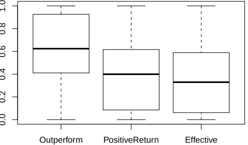
The results presented in this section are the average per-formance results for the ABBs over all test periods. There are three metrics considered: (1) the average number of ABBs that outperform the market (OM), (2) the average number of ABBs that produce a positive return (PR), and (3) the average number of ABBs that are effective (EF), where effective implies, from the above definition, that the ABB was profitable, active and outperformed the market index. The following sections will present tables and box plots of the results as well as a discussion.

1) Case 1 through Case 4: The results from training and testing the ABBs using sliding windows of 125, 250, 500 and 1000 days are presented in tables VI-IX and figures 4-7 are boxplots of the metric distributions.

E. Discussion

(8)

window Eff ectiv e 0.20 0.25 0.30 0.35 3 4 5 6 7 8 9 10 12

125 250 500 1000

T

rades

Effective Trades

[image:8.612.52.558.60.208.2]

Fig. 3. Plots of the average number of trades for effective ABBs and the average percentage of ABBs that were effective.

TABLE VI

THE RESULTS FROM TRAINING AND TESTING THEABBS WITH A SLIDING WINDOW OF125DAYS.??tr¯ STANDS FOR THE AVERAGE NUMBER OF

TRADES BY THEABBS THAT SATISFIED THE CONCERNED METRIC.

OM OMtr_¯ PR P Rtr¯ EF EFtr¯

[image:8.612.311.557.267.411.2]

Average 0.444 2.841 0.463 2.409 0.193 2.844 Min 0.116 0.000 0.000 0.000 0.000 1.000 Max 0.627 21.270 1.000 19.723 0.462 19.914 Median 0.449 1.941 0.434 1.549 0.192 1.984

TABLE VII

Average 0.438 5.128 0.371 4.588 0.162 4.829 Min 0.056 0.000 0.013 0.000 0.000 1.000 Max 0.678 41.695 1.000 38.571 0.422 38.147 Median 0.438 4.015 0.343 3.669 0.157 3.765

TABLE VIII

Average 0.601 8.558 0.311 6.689 0.226 6.521 Min 0.001 0.062 0.000 0.065 0.000 1.000 Max 0.959 92.201 0.997 92.028 0.858 92.028 median 0.617 7.258 0.289 5.463 0.219 5.123

TABLE IX

OM OM_tr_¯ _PR P R_tr_¯ _EF EF_tr_¯ Average 0.611 12.108 0.391 11.871 0.352 12.289 Min 0.000 0.000 0.000 0.000 0.000 1.000 Max 1.000 51.171 1.000 48.952 1.000 48.952 Median 0.624 13.593 0.399 13.296 0.329 13.589

data are more likely to become overfitted and to not generalize as well. We also observe a monotonic increase in the average number of trades executed by the ABBs as the window size increases. From the OM and PR metrics we can observe

● ● ● ● ● ● ● ● ● ● ● ● ● ● ● ● ● ● ● ● ● ● ● ● ● ● ● ● ● ● ● ● ● ● ● ● ● ● ● ● ● ● ● ● ● ● ● ● ● ● ● ● ● ● ● ● ● ● ● ● ● ● ● ● ● ● ● ● ● ● ● ● ● ● ● ● ● ● ● ● ● ● ● ● ● ● ● ● ● ● ● ● ● ● ● ● ● ● ● ● ● ● ● ● ● ● ● ● ● ● ● ● ● ● ● ● ● ● ● ● ● ● ● ● ● ● ● ● ● ● ● ● ● ● ● ● ● ● ● ● ● ● ● ● ● ● ● ● ● ● ● ● ● ● ● ● ● ● ● ● ● ● ● ● ● ● ● ● ● ● ● ● ● ● ● ● ● ● ● ● ● ●

Outperform PositiveReturn Effective

0.0 0.2 0.4 0.6 0.8 1.0

Fig. 4. Box plots of the distributions of the Outperform the Market (OM), Positive Return (PR) and EFfective (EF) metrics for case 1.

● ● ● ● ● ● ● ● ● ● ● ● ● ● ● ● ● ● ● ● ● ● ● ● ● ● ● ● ● ● ● ● ● ● ● ● ● ● ● ● ● ● ● ● ● ● ● ● ● ● ● ● ● ● ● ● ● ● ● ● ● ● ● ● ● ● ● ● ● ● ● ● ● ● ● ● ● ● ● ● ● ● ● ● ● ● ● ● ● ● ● ● ● ● ● ● ● ● ● ● ● ● ● ● ● ● ● ● ● ● ● ● ● ● ● ● ● ● ● ● ● ● ● ● ● ● ● ● ● ● ● ● ● ● ● ● ● ●

0.0 0.2 0.4 0.6 0.8 1.0

that ABBs are not always active in the market and that the parameters which are optimal in one time period can lead to a technical indicator that does not execute any trades when the market environment is quite different. This is partly the reason for higher percentages of the ABBs producing positive returns but not being able to outperform the market. On average the ABBs made a trade every 3 to 4 months when they were effective, though there were instances where the ABBs were effective and extremely active in executing trades. In case 3 where the window size was 500 days we observe a maximum average trading activity of 92.028, which translates to about 4 trades a month. This is quite active for a technical indicator that is identifying turning points in stocks price behaviour.

(9)

● ●

● ● ●

● ●

● ● ●

● ● ● ●

● ● ● ● ●

● ●

● ● ●

●

● ●

●

● ● ●

●

● ● ● ●

●

● ●

● ● ●

● ●

● ● ●

● ● ● ● ●

● ● ● ●

●

● ● ● ● ● ● ● ●

● ● ●

●

● ●

0.0

0.2

0.4

0.6

0.8

[image:9.612.47.295.60.209.2]

1.0

0.0

0.2

0.4

0.6

0.8

1.0

IV. CONCLUSIONS ANDFUTUREWORK

This paper presented an analysis of two implications of the AMH from a computational intelligence perspective. The first was variable efficiency and whether the presence of non-linear dependence in a time-series offered any advantages for fore-casting with supervised learning algorithms. The results clearly demonstrate that when non-linear dependence is present there is a statistically significant increase in the directional accuracy of the SL algorithms forecasts. This result was obtained using a simulated GARCH process but proves that if non-linear dependence can be reliably detected in a financial time-series then more accurate forecasts can be expected.

The second implication of cyclical profitability was shown to be quite abundant in the financial markets. Its more re-strictive form, cyclical effectiveness, was also shown to be valid though not as abundant. This result demonstrates that trading models fitted to one time-period will have a non-zero probability of being effective again. The results also provide insight into overfitting and the information content in older previously learned models.

Future work concerns the development of a forecasting algorithm which can combine the signals produced by a

population of optimized technical indicators to take advantage of cyclical profitability.

REFERENCES

[1] Matthew Butler and Dimitar Kazakov. Particle swarm optimization of bollinger bands. In Proceedings of the 7th international conference on Swarm intelligence, ANTS’10, pages 504–511, Berlin, Heidelberg, 2010. Springer-Verlag.

[2] Daniel O. Cajueiro and Benjamin M. Tabak. Ranking efficiency for emerging markets.Chaos, Solitons and Fractals, 22(2):349 – 352, 2004. [3] Rachel Caspari. The evolution of grandparents. Scientific American,

305:44–49, August 2011.

[4] Andries Engelbrecht. Heterogeneous particle swarm optimization. In Marco Dorigo, Mauro Birattari, Gianni Di Caro, Ren Doursat, Andries Engelbrecht, Dario Floreano, Luca Gambardella, Roderich Gro, Erol Sahin, Hiroki Sayama, and Thomas Sttzle, editors,Swarm Intelligence, volume 6234 of Lecture Notes in Computer Science, pages 191–202. Springer Berlin / Heidelberg, 2010.

[5] Eugene F Fama. Efficient capital markets: A review of theory and empirical work. Journal of Finance, 25(2):383–417, May 1970. [6] M. Hinich and D. Patterson. Detecting epochs of transient dependence

in white noise. Money, Measurement and Computation, pages 61–75, 2005.

[7] Carlos M. Jarque and Anil K. Bera. Efficient tests for normality, homoscedasticity and serial independence of regression residuals. Eco-nomics Letters, 6(3):255 – 259, 1980.

[8] J. Kennedy and R. Eberhart. Particle swarm optimization. InNeural Networks, 1995. Proceedings., IEEE International Conference on, vol-ume 4, pages 1942 –1948 vol.4, nov/dec 1995.

[9] Bjoern Krollner, Bruce Vanstone, and Gavin Finnie. Financial time series forecasting with machine learning techniques: A survey. InEuropean symposium on artificial neural networks: Computational and machine learning. Bruges, Belgium.Apr. 2010. School of Information Technology at ePublications@bond, 2010.

[10] Ju-Sang Lee, Sangook Lee, Seokcheol Chang, and Byung-Ha Ahn. A comparison of GA and PSO for excess return evaluation in stock markets. InIWINAC (2), pages 221–230, 2005.

[11] C. Lento and N. Gradojevic. The profitability of technical trading rules: a combined signal approach. Journal of Applied Business Research, 23(1):13–27, 2007.

[12] J. Leung and T. Chong. An empirical comparison of moving average envelopes and Bollinger Bands.Applied Economics Letters, 10(6):339– 341, 2003.

[13] Kian-Ping Lim. Ranking market efficiency for stock markets: A nonlin-ear perspective. Physica A: Statistical Mechanics and its Applications, 376:445 – 454, 2007.

[14] Andrew W. Lo. The adaptive markets hypothesis: market efficiency from an evolutionary perspective. Journal of Portfolio Management, 30:15–29, 2004.

[15] Andrew W. Lo. Reconciling efficient markets with behavioral finance: the adaptive markets hypothesis.Journal of Investment Consulting, 7:21– 44, 2005.

[16] J. Moody, L. Wu, Y. Liao, and M. Saffell. Performance functions and reinforcement learning for trading systems and portfolios. Applied Financial Economics Letters, 17:441–470, 1998.

[17] Y. Shi and R. Eberhart. A modified particle swarm optimizer. In Evolutionary Computation Proceedings, 1998. IEEE World Congress on Computational Intelligence., The 1998 IEEE International Conference on, pages 69–73, 1998.

[18] Alexandru Todea, Maria Ulici, and Simona Silaghi. Adaptive markets hypothesis - evidence from Asia-Pacific financial markets. The Review of Finance and Banking, 1(1):007–013, December 2009.

[19] Paul D. Yoo, Maria H. Kim, and Tony Jan. Machine learning techniques and use of event information for stock market prediction: A survey and evaluation. InCIMCA-IAWTIC’06, pages 835–841, Washington, DC, USA, 2005. IEEE Computer Society.

[image:9.612.49.296.258.403.2]