Uncertainty in geocentre estimates in the context of ITRF2014

This article has been accepted for publication and undergone full peer review but has not been through the copyediting, typesetting, pagination and proofreading process which may lead to differences between this version and the Version of Record. Please cite this article as doi: 10.1002/2016JB013698

Uncertainty in geocenter estimates in the context of ITRF2014

Anna R. Riddell1,2, Matt A. King1, Christopher S. Watson1, Yu Sun3, Riccardo E.M. Riva3 and Roelof Rietbroek4

1

Surveying and Spatial Sciences, School of Land and Food, University of Tasmania, Hobart, Tasmania, Australia.

2

Geoscience Australia, Canberra, Australia.

3

Department of Geoscience and Remote Sensing, Delft University of Technology, Delft, Netherlands.

4

Institute of Geodesy and Geoinformation,University of Bonn, Bonn, Germany.

Corresponding author: Anna Riddell ([email protected])

Key Points:

 Network translations from surface mass transport models cannot account for the variability in SLR translations

 We identify colored noise in SLR translations, increasing uncertainties in the rates 5-fold (upper bound) compared to white-noise only

 When using a power-law and white noise model the SLR Z rate uncertainty (±0.33 mm/yr; one sigma) is improved 27% since ITRF2008



Abstract

Uncertainty in the geocenter position and its subsequent motion affects positioning estimates on the surface of the Earth and downstream products such as site velocities, particularly the vertical component. The current version of the International Terrestrial Reference Frame, ITRF2014, derives its origin as the long-term averaged center of mass as sensed by Satellite Laser Ranging (SLR), and by definition, it adopts only linear motion of the origin with uncertainty determined using a white noise process. We compare weekly SLR translations relative to the ITRF2014 origin, with network translations estimated from station

displacements from surface mass transport models. We find that the proportion of variance explained in SLR translations by the model-derived translations is on average less than 10%. Time-correlated noise and non-linear rates, particularly evident in the Y and Z components of the SLR translations with respect to the ITRF2014 origin, are not fully replicated by the model-derived translations. This suggests that translation-related uncertainties are

underestimated when a white noise model is adopted, and that substantial systematic errors remain in the data defining the ITRF origin. When using a white noise model, we find uncertainties in the rate of SLR X, Y and Z translations of ±0.03, ±0.03 and ±0.06

1 Introduction

The need to monitor global change processes, such as sea-level change and

postglacial rebound, at a level below 1 mm per year illustrates the requirement for an accurate and precise global geodetic reference frame. The International Terrestrial Reference Frame (ITRF) [Altamimi et al., 2016] attempts to meet accuracy and stability goals of 1 mm and 0.1 mm/yr respectively [Gross et al., 2009]. As each iteration of the ITRF provides

improvements in the precision and accuracy of the global reference frame, challenges remain to meet the accuracy and stability goals. Particularly challenging is the realization of the origin (defined as the long-term averaged center of mass (CM) of the Earth), and its evolution in time [Dong et al., 2014]. Presently, this realization is limited given it is determined using measurements from a single measurement technique [Satellite Laser Ranging (SLR),

Altamimi et al., 2016; Wu et al., 2011] that is known to be affected by systematic biases and network asymmetry [Appleby et al., 2016]. The ITRF2014 (and each predecessor) is a linear frame by definition, and consequently the long-term motion of its origin is described by a linear trend. Limitations arise given that when specifying the ITRF origin to coincide with the long-term origin of the SLR frame, only time-constant annual and semi-annual terms are included with a white noise model [Altamimi et al., 2007; 2011; 2016; Argus, 2012], neglecting any other non-linear motions as part of the functional or stochastic model.

Relative motion between the Centre of Mass of the total Earth system (CM) and the Centre of surface Figure (CF) of the solid Earth can be observed using space geodetic

observations that tie Earth-fixed permanent geodetic sites and space-based satellite platforms. Both secular and seasonal geocenter motion occurs as a result of past and present mass re-distribution, where geocenter motion is the difference between CM and CF (the difference between geophysically determined origins). Past mass redistribution on the surface or interior such as glacial isostatic adjustment (GIA), induces secular geocenter motion, while intra-annual, seasonal and inter-annual signals relate to present day distributions, such as exchanges within and between the ocean, atmosphere, continents and cryosphere [Argus,

2012; Dong et al., 1997; Wu et al., 2012]. SLR translations with respect to the ITRF2014 origin therefore consist of both measurement error and a component of real geocenter motion affected by the non-homogenous network distribution of SLR tracking stations. This leads to a sampling bias known as the “network effect”, and should ideally reflect the offset between the network origin (CN) and the CM rather than the geocenter motion.

An alternative approach to studying geocenter motion uses observations and numerical models of surface mass transport to derive deformation of the solid Earth at the locations of the SLR stations (that change over time), from which network translations may be estimated. The mass transport models provide bounds on the network translations which are to be expected from known surface loading processes. Any inconsistency between observed SLR translations and those derived from a surface loading model will hint at problems in either the SLR methods (observations or processing) or problems within the surface loading model. In this paper, SLR translations and output from two surface loading models are used to assess the uncertainty in the SLR translations with respect to the

ITRF2014 long-term origin.

2 Data

defined using the internal constraint method described in Altamimi et al. [2007] and Altamimi et al. [2016]. The translations were estimated using a 7-parameter similarity transformation between each week and a SLR ITRF2014 network of 21 core stations. The time series of the 7-parameters were adjusted globally, in one run using the CATREF software [Combination and Analysis of Terrestrial Reference Frames, e.g. Altamimi et al., 2016], with the full variance-covariance information of the total SLR SINEX time series. We analyze the translations from weekly combined SLR solutions relative to the ITRF2014 (linear) origin over the time span 1993.0 to 2015.0 in the temporal and spectral domains. The complete ILRS SLR reference frame solutions in SINEX format submitted for the realization of ITRF2014 covers the time span 1983.0 to 2015.0. Only the data from 1993.0 onwards are used here due to noisy data in the early section of the time series, producing large formal uncertainties in the SLR translation series before the LAGEOS-2 satellite was launched in 1992 [Dong et al., 2014]. We compare the SLR translation time series with respect to the ITRF2014 long-term origin with two different estimates of network translations that are derived from independent surface mass transport models.

The ITRF2014 origin is considered theoretically representative of the long-term CM, where geocentre motion is defined as motion of the CM with respect to the CF [Altamimi et al., 2016]. Linear motions for ground stations are assumed, with some discontinuities and post-seismic deformations enforced for sites affected by major earthquakes or equipment changes. The ITRF origin reflects CM on secular time scales due to it coinciding with the long-term average CM as observed by SLR, but on shorter (including seasonal) time scales, the ITRF origin reflects CF [Blewitt, 2003; Collilieux et al., 2009; Dong et al., 2003]. We note that some of the literature considers the opposite convention, that is, displacement of CF with respect to CM, for example Métivier et al. [2010] and Dong et al. [2014].

Our first comparative geophysical model is from Rietbroek et al. [2015], who calculated surface mass transport loading based on a combination of GRACE and radar altimetry data using an inversion approach that applied conservation of mass to solve the sea level equation [Rietbroek et al., 2016]. Surface displacement components are provided for the time span 2002.3 to 2014.5 with monthly sampling, here-on referred to as R15. R15 considers mass redistribution from the Antarctic and Greenland ice sheets, land glaciers, GIA,

continental water storage, and contributions from the oceans and atmosphere. Although GRACE alone is not capable of observing degree-1 mass redistribution, combination with additional datasets and use of an inversion methodology enables derivation of surface mass transport values. The short data span is limiting given it covers only half of the SLR series, but remains useful given the independent GRACE-based approach.

Our second dataset was estimated from numerical surface mass transport models and solves the sea level equation to conserve mass for the global system after taking into account self-attraction and loading effects [Gordeev et al., 1977; Frederikse et al., 2016; Tamisiea et al., 2010] using fingerprints [Mitrovica et al., 2001] to represent the non-uniform

interpolated to monthly intervals for consistency with the other datasets, constraining the temporal resolution. It would be expected for these components to contain annual signals due to the seasonal nature of hydrologic mass exchange, and we return to this in the Discussion. A groundwater component is available using data from Wada et al. [2010]. The contribution from groundwater to the overall signal is primarily linear with very small annual amplitude for the available period. Further data description for MSM is available in the Supporting Information (Text S1) and Frederikse et al. [2016], including uncertainties for the component contributions.

Surface displacements from each geophysical model were derived by redistributing loaded masses within a thin shell on the Earth’s surface. They are spherically symmetric, stratified, and non-rotating Earth responses elastically redistributed over sub-secular (sub-daily to decadal) time scales. The displacements are proportional to the incremental load potential according to the load Love number theory [Farrell, 1972], and are derived from the PREM elastic Earth model [Dziewonski et al., 1981].

Following the methodology of Collilieux et al. [2009], network translations have been derived from station displacements due to loading effects from two distinct surface mass transport models and compared with SLR translations with respect to the ITRF2014 long-term origin to account for the network effect of the SLR station geometry.

From each of the geophysical models, network translations are computed following the methodology of Collilieux et al. [2009], using the ITRF2014 station positions and

velocities plus the modelled surface mass loading deformation at each epoch of the respective dataset. At each epoch, we used only those SLR sites that were active. The monthly surface deformation values are interpolated from monthly to weekly values using a cubic spline. The two synthetic time series are then used to estimate transformation parameters, using Globk [Herring et al., 2015], with respect to ITRF2014 using the full covariance matrix of the ILRS combined solution submitted for ITRF2014 analysis. Following Collilieux et al. [2012], only three rotations and three translations were estimated (that is, scale was not estimated).

Repeating the analysis with the scale parameter included produced only negligible changes to the estimated transformation parameters. Covariance information was used as given; an occasional site was automatically removed for a given week due to the estimated station adjustments being larger than 10-sigma. Given that the ILRS combined solution was generated using a loose constraint approach correlations exist between the Helmert parameters, some of the station displacements may leak into the rotation parameters

[Collilieux et al., 2009]. Here, the rotations have a mean and standard deviation of 0.00±0.02 mas for all components from both models (one sigma), which induces station displacements below 1 mm.

The two network translation models, R15 and MSM are compared with the SLR translation components with respect to the ITRF2014 origin to assess the sensitivity of the SLR observed origin against geophysically modeled geocenter motion taking into account the network effect of the SLR observing network.

3 Comparison of SLR and modelled network translations

By construction, there are zero translation rates (trends) between ITRF2014 and the SLR stacked frame of weekly solutions over the time span 1993.0 to 2015.0. Annual and semi-annual periodic signals were not removed from the SLR translation components as these are signals of interest. Figure 1 (left) shows the three datasets in the temporal domain

either of the surface mass transport models, but uncertainties are available for the constituent datasets that contribute to each model. Further information on the model uncertainties can be found in the associated references. Our use of two geophysical models aims to reflect, at least partly, the uncertainty in the two models.

Figure 1 (right) shows the SLR translations alongside the differences of R15 and MSM with SLR, where the qualitative agreement of the curves reveal that the differences are heavily influenced by signal not in R15 and MSM. Considering the residual series, the percentage of SLR variance explained by R15 is 12.5%, 1.3% and 2.1% for the X, Y, Z components, respectively, with MSM explaining 8.1%, 4.0% and 2.0%, respectively. The small proportion of variance explained by the surface mass transport models indicates that either the geophysical models are not able to capture the surface mass transport variability and/or systematic errors from the SLR technique are substantial. The visual agreement between R15 and MSM is noteworthy given the dissimilarity in the data used to construct the series. Surface thermoelastic effects, with annual amplitudes approaching 3 mm for radial displacements and 1.5 mm for transverse displacements [Xu et al., 2017], could explain some of the difference between the SLR translations and the respective network translations.

3.1 Seasonal variation

The dominant signal throughout the SLR translation series has an annual period with apparent variable amplitude. Over the full time series, the SLR translation annual signal in the Z component is approximately twice that of the SLR translation X and Y components (see Table 1). The greatest agreement in overall amplitude and its temporal variation between SLR, R15 and MSM is found in the X component, which is predominantly ocean-driven due to the limited land area along the X axis (X is in the direction of 0°N 0°E, Y of 0°N, and Z of 90°N).

The annual signal expressed in the residuals for each coordinate component (Figure 1d, e, f, SLR minus model) computed between the SLR origin and model based network translation estimates, demonstrate reasonable qualitative agreement in phase and amplitude, again demonstrating that both the R15 and MSM models significantly underestimate the amplitude of the annual signal within the SLR translations. To explore the strength of the annual signals more closely we computed the Power Spectral Density (PSD) using the Lomb-Scargle approach described by Press et al. [1992]. Figure 2 shows the PSD for each dataset across each coordinate component. Lower frequency trends are less well resolved by R15 due to the restricted temporal span, and care should be taken not to over-interpret differences at these frequencies.

The annual signal expressed in MSM significantly underestimates the observed SLR amplitude in all components, particularly during the latter part of the Y component time series (Figure 1b) and remains visible as a peak in the residual PSD (Figure 2e). The shorter duration R15 model also underestimates the magnitude of the annual signal, where the most notable differences for both R15 and MSM are with respect to the Z component (Figure 1c). This is confirmed by the presence of a residual peak at the one cycle per year frequency in the bottom panels of Figure 2.

That the surface mass transport models are indistinguishable from each other in the later part of the time series provides confidence in their construction, noting again the dissimilarities in their constituent data series.

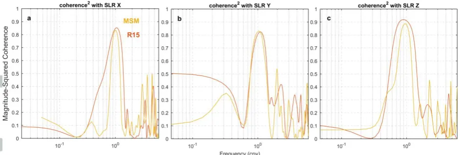
The magnitude-squared coherence of the SLR time series with each of the models in Figure 3, provides further evidence that an annual signal is clearly present in both the observations from SLR and the network translation estimates from geophysical models. A strong peak in each component is centered about one cycle per year, with an average magnitude-squared coherence of 0.9 across the X, Y and Z components. Figure 3a shows agreement in the X component is poor for signals other than annual, particularly between SLR and R15. Better agreement at other frequencies is evident in the Y and Z components between SLR and the network translation models. Other less significant peaks are observed at sub-annual periods, but they are not considered further here.

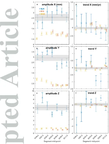
To assess the time-variability of the time series, we follow a similar method to Argus

[2012] whereby each time series is divided into four-year segments, each overlapping by one year, producing seven segments in our analysis. A linear plus seasonal model was fitted to each segment, with the amplitude for each origin component shown in Figure 4a, b, c, each centered on the mid-point of the segment. Four years is sufficient to reliably estimate the linear plus annual and semi-annual terms [Blewitt and Lavallee 2002]. For the SLR data, a number of annual amplitudes computed from segmented data are significantly different to those computed over the full series in the Y and Z components. While natural variation in these terms is expected, some of the behavior appears systematic and specific to SLR. For example, the Y component shows a marked reduction in amplitude following the segment centered on 2003.5 (Figure 4b), which is not reflected in the R15 data, and only marginally reflected in the MSM data. The largest variability in SLR annual amplitude is found in the Z component (Figure 4c), with the large deviation in the segment centered on 1997.5 not reproduced by either R15 or MSM.

We also note a decrease in the uncertainty of the annual amplitude across the SLR data segments, most noticeably in the X and Z components. This perhaps reflects refinements in the SLR observing networks’ geometry and operation capacity over time [Varghese, 2013].

3.2 Noise characteristics

Examination of Figure 2 shows clear features other than the dominant annual signals. The noise floor of the SLR dataset is substantially higher than that of both the network translation models, presumably associated the effect of measurement error. The SLR X component (Figure 2a) shows a flatter (whiter) spectrum than in Y and Z indicating increased time-correlated noise in the latter components. The spectra of SLR-R15 and SLR-MSM (Figure 2 d, e, f) also suggests time-correlated noise across each component.

The uncertainty in the rate of the SLR translations, estimated with a PLW noise model over the complete time span, is a factor of five larger in comparison to a white noise-only model (see Table 1). That is, white noise uncertainties for X, Y and Z rates respectively of ±0.03, ±0.03 and ±0.06 increase to ±0.13, ±0.17 and ±0.33 (mm/yr) when a PLW noise model is adopted. A PLW noise model was chosen instead of GGM for the remaining analysis as a conservative estimate of rate uncertainty. We examined the apparent offset around 2010 in the SLR origin Y component (Figure 1b, e), as described by Altamimi et al.

[2016], and found it to be statistically insignificant when estimated as an offset within the noise analysis. Neither of the geophysical models show an offset at this time. Together, this suggests that the apparent discontinuity is simply characteristic of power law time-correlated noise with spectral indices close to -1 (flicker noise) [Williams, 2003]. No other offsets were estimated for the datasets.

Neither of the network translations from the geophysical models capture the long period variability in the SLR series particularly well. The removal of the models from the SLR series results in generally no change to the spectral index for the PLW model in the X, Y and Z components for both MSM and R15, (see Table 1 and Table 2).

3.3 Time-variable trends

We next consider the multi-year trends in the SLR translation time series. By convention, the linear rate of each SLR origin translation component are not statistically different from zero [Altamimi et al., 2016] over the full time series. However, low frequency variability is evident in the SLR time series, particularly in the Y and Z components (Figure 1b, c). This signal is not present in either of the mass transport models (Figure 1, noting the same scale is used in the left and right panels). The non-linear signature observed in the temporal domain of the SLR Y component in Figure 1b is similarly reflected in Figure 2b where the Y component of the SLR origin series shows high power at low frequencies.

The time-variable rate within each data series is shown in Figure 4d, e, f, for each of the four-year segments discussed previously. Similarly to the annual amplitude, the largest temporal variability in the short-term rate is found in the SLR Y and Z components (Figure 4e, f), with a number of short-term rates significantly different to the rate determined over the full record (grey line, Figure 4d, e, f). The section of the SLR X and Z components before 1997.0 are distinctly different from the long-term average, with the Z component almost a factor of three larger than the long-term mean in this period. Segments in the Y component have differences from the mean ranging from +0.8 mm/yr to -0.9 mm/yr, and the two segments covering 2005.0 – 2012.0 are statistically significant from the long-term average. R15 contains contributions from ocean mass and ice sheets mass that are indirectly affected by the GIA model used, which are not included in MSM and could explain some of the offset between the rates derived from the two models.

4 Discussion

Our comparison of the SLR translations with respect to the ITRF2014 origin with network translations derived from equivalently sampled geophysical models shows that it is likely that signals of non-geophysical origin, with a range of frequencies (monthly to inter-annual) are insufficiently accounted for in the stochastic model of the ITRF2014 origin.

Several studies have examined potential systematic error in SLR, in particular the influence of the time-variable ground network distribution [Collilieux et al., 2009; Collilieux and Wöppelmann, 2011], and satellite observation geometry [Spatar et al., 2015] in order to assess uncertainty. Collilieux et al. [2009] found that the SLR network effect could affect the amplitude of the annual geocenter motion in the Z direction at approximately 1-mm,

depending on the simulated observing network geometry. We found that the network effect was dominated by the geophysical models’ annual signal, rather than the network geometry and account for the SLR network effect by deriving network translations from geophysical models, using only the surface deformation at those active SLR stations for each epoch.

Previous studies have explored uncertainty in the data series submitted to the previous ITRF, ITRF2008 [Altamimi et al., 2011], and found substantial non-linear variation around the origin [Métivier et al., 2010; Argus, 2012]. Dong et al. [2014] notes an acceleration in the Z geocenter component of the ITRF2008 origin after 1998, and attributes this to terrestrial water mass redistribution, including mass loss from continental ice sheets and glaciers. We note the same feature in our analysis with a clear change in the short-term rate of the SLR Z component (Figure 4f), but note this is not replicated by MSM, even though MSM and Dong et al., [2014] both use the GLDAS terrestrial water storage model. We note there are

differences in the glacier and ice sheet mass terms which could explain why the deviation is not present in MSM; the reason for this discrepancy requires further consideration.

Both the land glacier and dam retention components of the MSM surface mass transport model have insufficient temporal resolution to capture the annual component of these constituents. The resolution of surface displacements due to terrestrial water storage changes remains challenging due to deficiencies in hydrologic models, in particular the long-term trends and accurate representation of groundwater use. The missing annual hydrologic signal could explain some of the gap between SLR and MSM, but we note that this signal is included in R15 which also does not agree with SLR in amplitude over a short period.

Others have evaluated the stability of the ITRF2008 origin using statistical and spectral analysis [Collilieux and Altamimi, 2013; Argus 2012]. These analyses show that a colored noise model is more appropriate than a white noise-only model, an outcome that we find remains robust for the ITRF2014 origin. Argus [2012] demonstrated time-variability in both the annual amplitude and short-term rates of geocenter motion and that the linear CM velocity uncertainties are ±0.4 mm/yr for X and Y and ±0.9 mm/yr for the Z component (95% confidence limit). Our findings confirm that a simple linear regression using a white noise-only model will poorly reflect the true uncertainty of the estimated parameters, with the uncertainty for the linear rate typically a factor of five smaller than estimates using a PLW noise model (see Table 1 and Table 2). Our analysis of the SLR translations relative to the ITRF2014 origin suggests improvement of the CM velocity compared with those from Argus,

[2012] for ITRF2008. Simply scaling our rate uncertainties to 2 sigma, the PLW noise model results in a 27% improvement of the SLR Z component, reducing from ±0.9 mm/yr (95% confidence limit) [Argus, 2012] to ±0.66 mm/yr (95% confidence limit).

The future improvement of the precision and accuracy of the ITRF origin will depend on advances in analysis of SLR data and improved network geometry. Indeed, the present SLR station geometry is sub-optimal, with a concentration of SLR stations in the northern hemisphere decreasing the precision of the Z component compared to the equatorial components [Bouillé et al., 2000; Collilieux and Wöppelmann, 2011; Wu et al., 2012].

component of the geocenter, and that additional sites at high latitudes, particularly in the south, would provide an important improvement in the X and Y geocenter components.

5 Conclusions

We assess the temporal variability of the latest SLR translations with respect to the International Terrestrial Reference Frame (ITRF2014) origin, and find significant differences when compared to modeled network translations from two independent surface mass

transport models. The proportion of variance explained in the SLR origin time series by geophysical models is on average less than 10% in each component. We identified colored noise in both observed and modelled network translation time series, but substantial colored noise remains after subtraction of the model based translations, with notable signal remaining at annual and longer periods. Consideration of power-law noise when estimating the rate in the origin components yields an upper bound five-fold increase in rate uncertainty, compared to the white noise-only case. When using a power-law and white model the uncertainty of the SLR Z component (0.33 mm/yr; 1 sigma) is twice as large as that of the X and Y components (0.13 and 0.17 mm/yr respectively). This represents a 27% improvement for the Z component of the results in comparison to those from Argus [2012] for ITRF2008.

Over shorter time-periods, the temporal variability of linear rates computed over four years suggests that the SLR translations with respect to the long-term ITRF2014 origin cannot be rigorously represented by a simple linear model over longer periods. For the annual signal, model based network translations, particularly in the Z component, do not represent the variability in the annual amplitude of the SLR translations with respect to the ITRF2014 origin. This indicates that a significant component of the signal is due to other processes, including likely large systematic error.

Positioning uncertainty for geophysical applications is likely to be impacted by non-linear geophysical signals of the kind we identify in the SLR translation time series with respect to the ITRF2014 origin, and may be further impacted when non-geophysical signals exist. Space geodetic analyses that require an instantaneous CM frame (precise orbit

determination for example) will also likely be affected given the annual geocenter motion model used is derived from the same SLR data that is used to define the long-term origin of ITRF2014. Further improvements in SLR data analysis and network geometry are likely required to address this issue. The demonstration of other geodetic techniques to contribute to the Earth’s center of mass determination would also be of great benefit.

Acknowledgments, Samples, and Data

References

Akaike, H. (1973), Information theory and an extension of the maximum likelihood principle. In B. N. Petrov & B. F. Csaki (Eds.),Second International Symposium on Information Theory, 267–281, Academiai Kiado: Budapest.

Altamimi, Z., X. Collilieux, J. Legrand, B. Garayt, and C. Boucher (2007), ITRF2005: A new release of the International Terrestrial Reference Frame based on time series of station positions and Earth Orientation Parameters, J. of Geophys. Res. Solid Earth, 112(B9), doi:10.1029/2007JB004949.

Altamimi, Z., X. Collilieux, and L. Métivier (2011), ITRF2008: An improved solution of the international terrestrial reference frame, J Geod., 85(8), 457-473, doi:10.1007/s00190-011-0444-4.

Altamimi, Z., P. Rebischung, L. Métivier, and X. Collilieux (2016), ITRF2014: A new release of the International Terrestrial Reference Frame modeling non-linear station motions, J. of Geophys. Res. Solid Earth, 121, doi:10.1002/2016JB013098.

Appleby, G., J. Rodríguez, and Z. Altamimi (2016), Assessment of the accuracy of global geodetic satellite laser ranging observations and estimated impact on ITRF scale: estimation of systematic errors in LAGEOS observations 1993–2014, J Geod., 1-18, doi:10.1007/s00190-016-0929-2.

Argus, D. F. (2012), Uncertainty in the velocity between the mass center and surface of Earth, J. of Geophys. Res. Solid Earth, 117(B10), 1-15, doi:10.1029/2012JB009196.

Blewitt, G., and D. Lavallée (2002), Effect of annual signals on geodetic velocity, J. of Geophys. Res. Solid Earth, 107(B7), ETG 9-1-ETG 9-11, doi:10.1029/2001jb000570.

Bos, M. S., R. M. S. Fernandes, S. D. P. Williams, and L. Bastos (2013), Fast error analysis of continuous GNSS observations with missing data, J Geod., 87(4), 351-360, doi:10.1007/s00190-012-0605-0.

Bouillé, F., A. Cazenave, J. M. Lemoine, and J. F. Crétaux (2000), Geocentre motion from the DORIS space system and laser data to the LAGEOS satellites: comparison with surface loading data, Geophys. J. Int., 143(1), 71-82,

doi:10.1046/j.1365-246x.2000.00196.x.

Chao, B. F., Y. H. Wu, and Y. S. Li (2008), Impact of Artificial Reservoir Water Impoundment on Global Sea Level, Science, 320(5873), 212-214,

doi:10.1126/science.1154580.

Chen, J. L., C. R. Wilson, R. J. Eanes, and R. S. Nerem (1999), Geophysical interpretation of observed geocenter variations, J. of Geophys. Res. Solid Earth, 104(B2), 2683-2690, doi:10.1029/1998JB900019.

Cheng, M. K., J. C. Ries, and B. D. Tapley (2013), Geocenter Variations from Analysis of SLR Data, in Reference Frames for Applications in Geosciences, edited by Z. Altamimi and X. Collilieux, pp. 19-25, Springer Berlin Heidelberg, Berlin, Heidelberg, doi:10.1007/978-3-642-32998-2_4.

Collilieux, X., Z. Altamimi, J. Ray, T. van Dam, and X. Wu (2009), Effect of the satellite laser ranging network distribution on geocenter motion estimation, J. of Geophys. Res. Solid Earth, 114(B04402), doi:10.1029/2008JB005727.

Collilieux, X., and G. Wöppelmann (2011), Global sea-level rise and its relation to the terrestrial reference frame, J Geod., 85(1), 9-22, doi:10.1007/s00190-010-0412-4.

Collilieux, X., T. van Dam, J. Ray, D. Coulot, L. Métivier, and Z. Altamimi (2012), Strategies to mitigate aliasing of loading signals while estimating GPS frame parameters, J Geod., 86(1), 1-14, doi:10.1007/s00190-011-0487-6.

Dong, D., J. O. Dickey, Y. Chao, and M. K. Cheng (1997), Geocenter variations caused by atmosphere, ocean and surface ground water, Geophys. Res. Lett., 24(15), 1867-1870, doi:10.1029/97GL01849.

Dong, D., W. Qu, P. Fang, and D. Peng (2014), Non-linearity of geocentre motion and its impact on the origin of the terrestrial reference frame, Geophys. J. Int., 198(2), 1071-1080, doi:10.1093/gji/ggu187.

Dong, D., T. Yunck, and M. Heflin (2003), Origin of the International Terrestrial Reference Frame, J. of Geophys. Res. Solid Earth, 108(B4), doi:10.1029/2002JB002035.

Dziewonski, A. M., and D. L. Anderson (1981), Preliminary reference Earth model, ‎Phys. Earth Planet. Inter, 25(4), 297-356, doi:10.1016/0031-9201(81)90046-7.

Farrell, W. E. (1972), Deformation of the Earth by surface loads, ‎Rev. Geophys, 10(3), 761-797, doi:10.1029/RG010i003p00761.

Flechtner, F., H. Dobslaw, and E. Fagiolini (2015), AOD1B product description document for product release 05 (Rev. 4.3) Technical Report, GFZ German Research Center for Geosciences, Postdam.

Frederikse, T., R. Riva, M. Kleinherenbrink, Y. Wada, M. van den Broeke, and B. Marzeion (2016), Closing the sea level budget on a regional scale: trends and variability on the Northwestern European continental shelf, Geophys. Res. Lett.,

doi:10.1002/2016GL070750.

Gordeev, R. G., B. A. Kagan, and E. V. Polyakov (1977), The Effects of Loading and Self-Attraction on Global Ocean Tides: The Model and the Results of a Numerical Experiment, J. Phys. Oceanogr., 7(2), 161-170,

doi:10.1175/1520-0485(1977)007<0161:TEOLAS>2.0.CO;2.

Gross, R., G. Beutler, and H.-P. Plag (2009), Integrated scientific and societal user requirements and functional specifications for the GGOS, in Global Geodetic Observing System: Meeting the Requirements of a Global Society on a Changing Planet in 2020, edited by H.-P. Plag and M. Pearlman, pp. 209-224, Springer Berlin Heidelberg, Berlin, Heidelberg, doi:10.1007/978-3-642-02687-4_7.

Herring, T., M. A. Floyd, R. W. King, and S. McClusky (2015), Globk Reference Manual, Global Kalman filter VLBI and GPS analysis program, Release 10.6, Massachusetts Institute of Technology.

Lehner, B., et al. (2011), High-resolution mapping of the world's reservoirs and dams for sustainable river-flow management, Front. Ecol. Environ., 9(9), 494-502,

Marzeion, B., P. W. Leclercq, J. G. Cogley, and A. H. Jarosch (2015), Brief Communication: Global reconstructions of glacier mass change during the 20th century are consistent, The Cryosphere, 9, 2399–2404, doi:10.5194/tc-9-2399-2015.

Métivier, L., M. Greff-Lefftz, and Z. Altamimi (2010), On secular geocenter motion: The impact of climate changes, Earth Planet. Sci. Lett., 296(3–4), 360-366,

doi:http://dx.doi.org/10.1016/j.epsl.2010.05.021.

Mitrovica, J. X., M. E. Tamisiea, J. L. Davis, and G. A. Milne (2001), Recent mass balance of polar ice sheets inferred from patterns of global sea-level change, Nature,

409(6823), 1026-1029,

doi:http://www.nature.com/nature/journal/v409/n6823/suppinfo/4091026a0_S1.html.

Noël, B., W. J. van de Berg, E. van Meijgaard, P. Kuipers Munneke, R. S. W. van de Wal, and M. R. van den Broeke (2015), Evaluation of the updated regional climate model RACMO2.3: summer snowfall impact on the Greenland Ice Sheet, The Cryosphere, 9(5), 1831-1844, doi:10.5194/tc-9-1831-2015.

Otsubo, T., K. Matsuo, Y. Aoyama, K. Yamamoto, T. Hobiger, T. Kubo-oka, and M. Sekido (2016), Effective expansion of satellite laser ranging network to improve global geodetic parameters, Earth, Planets and Space, 68(1), 1-7, doi:10.1186/s40623-016-0447-8.

Press, W. H., S. A. Teukolsky, W. T. Vetterling, and B. P. Flannery (1992), Numerical recipes in C (2nd ed.): the art of scientific computing, 994 pp., Cambridge University Press.

Rietbroek, R., S.-E. Brunnabend, J. Kusche, J. Schröter, and C. Dahle (2015), Global and Regional Sea level budget components from GRACE and radar altimetry (2002-2014), in Supplement to: Rietbroek, Roelof; Brunnabend, Sandra-Ester; Kusche, Jürgen; Schröter, Jens; Dahle, Christoph (2016): Revisiting the Contemporary Sea Level Budget on Global and Regional Scales. Proceedings of the National Academy of Sciences, 113, 1504-1509., doi:10.1073/pnas.1519132113, edited, PANGAEA, doi:10.1594/PANGAEA.855539.

Rietbroek, R., S.-E. Brunnabend, J. Kusche, J. Schröter, and C. Dahle (2016), Revisiting the contemporary sea-level budget on global and regional scales, Proc. Natl. Acad. Sci. U.S.A., 113(6), 1504-1509, doi:10.1073/pnas.1519132113.

Rodell, M., et al. (2004), The Global Land Data Assimilation System, Bull. Am. Meteorol. Soc., 85(3), 381-394, doi:10.1175/BAMS-85-3-381.

Schwarz, G. (1978), Estimating the Dimension of a Model, Ann. Statist., 6(2), 461-464, doi:10.1214/aos/1176344136.

Spatar, C. B., P. Moore, and P. J. Clarke (2015), Collinearity assessment of geocentre coordinates derived from multi-satellite SLR data, J Geod., 89(12), 1197-1216, doi:10.1007/s00190-015-0845-x.

Tamisiea, M. E., E. M. Hill, R. M. Ponte, J. L. Davis, I. Velicogna, and N. T. Vinogradova (2010), Impact of self-attraction and loading on the annual cycle in sea level, J. Geophys. Res. Oceans, 115(C7), doi:10.1029/2009JC005687.

Varghese, T. (2013), Engineering Changes to the NASA SLR Network to Overcome Obsoleteness, Improve Performance and Reliability, paper presented at Eighteenth International Workshop on Laser Ranging Instrumentation, Fujiyoshida, Japan.

Wada, Y., L. P. H. van Beek, C. M. van Kempen, J. W. T. M. Reckman, S. Vasak, and M. F. P. Bierkens (2010), Global depletion of groundwater resources, Geophys. Res. Lett., 37(20), doi:10.1029/2010GL044571.

Williams, S. D. P. (2003), Offsets in Global Positioning System time series, J. of Geophys. Res. Solid Earth, 108(B6), doi:10.1029/2002JB002156.

Wu, X., X. Collilieux, Z. Altamimi, B. L. A. Vermeersen, R. S. Gross, and I. Fukumori (2011), Accuracy of the International Terrestrial Reference Frame origin and Earth expansion, Geophys. Res. Lett., 38(13), doi:10.1029/2011GL047450.

Wu, X., J. Ray, and T. van Dam (2012), Geocenter motion and its geodetic and geophysical implications, J. Geodyn., 58, 44-61, doi:http://dx.doi.org/10.1016/j.jog.2012.01.007.

Xu, X., D. Dong, M. Fang, Y. Zhou, N. Wei, and F. Zhou (2017), Contributions of

Table 1. Noise parameters from HECTOR of the full SLR dataset and MSM network translation model [1993.0 2015.0]. AIC is a measure of the relative quality of statistical models for a given set of data; BIC is a criterion for model selection among a finite set of models; the model with the lowest AIC/BIC value is preferred; k is the spectral index; 1-phi is a GGM parameter; STD is the standard deviation (units mm).

X

SLR MSM SLR-MSM

model white-only PLW GGM white-only PLW GGM white-only PLW GGM

AIC 1323.350 1282.103 1256.500 438.639 393.762 392.735 1225.414 1204.903 1198.35 BIC 1323.350 1289.263 1263.659 438.639 400.921 399.894 1225.414 1212.062 1205.51

k 0 -0.80 0.98 ±

0.30 0 -0.59

0.62 ±

0.30 0 -0.50 0.47 ± 0.18

1-phi 0.51 ±

0.14

0.02 ±

0.03 0.36 ± 0.19

STD 2.939 2.689 2.570 0.504 0.5041 0.554 2.443 2.3301 2.303 bias (mm) -0.000 ± 0.181 -0.197 ± 2.123 -0.014 ± 0.306 0.005 ± 0.034 0.042 ± 0.173 0.025 ± 0.098 0.001 +/- 0.150 -0.102 +/- 0.602 -0.003 +/- 0.229 trend

(mm yr-1)

-0.000 ± 0.028 0.017 ± 0.128 0.000 ± 0.048 -0.001 ± 0.005 -0.009 ± 0.016 -0.007 ± 0.014 -0.005 +/- 0.024 0.007 +/- 0.061 -0.003 +/- 0.036 Y

AIC 1371.096 1222.215 1192.371 401.992 243.008 225.826 1193.983 1060.86 1064.138 BIC 1371.096 1229.374 1199.531 401.992 250.167 232.986 1193.983 1068.019 1071.297

k 0 -0.98 0.98 ±

0.13 0 -0.98

0.77 ±

0.11 0 -0.94 0.36 ± 0.04

1-phi 0.29 ±

0.08

0.17 ±

0.08 0.01 ± 0.01

STD 3.216 2.391 2.275 0.517 0.3769 0.367 2.302 1.7056 1.786 bias (mm) -0.000 ± 0.198 -0.451 ± 8.952 -0.024 ± 0.473 0.008 +/- 0.032 0.085 +/- 1.318 0.025 +/- 0.088 0.001 +/- 0.141 -0.374 +/- 2.525 -0.218 +/- 0.567 trend

(mm yr-1)

0.000 ± 0.031 -0.027 ± 0.166 -0.008 ± 0.073 0.000 +/- 0.005 -0.007 +/- 0.026 -0.002 +/- 0.013 0.006 +/- 0.022 0.003 +/- 0.082 0.002 +/- 0.069 Z

AIC 1761.462 1638.007 1585.610 367.806 318.881 316.801 1626.136 1512.313 1508.971 BIC 1761.462 1645.166 1592.769 367.806 326.04 323.96 1626.136 1519.473 1516.13

k 0 -0.93 1.48 ±

0.32 0 -0.66

0.37 ±

0.07 0 -0.86 0.49 ± 0.07

1-phi 0.48 ±

0.10

0.05 ±

0.06 0.05 ± 0.04

STD 6.717 5.252 4.777 0.484 0.4375 0.436 5.203 4.1494 4.135 bias (mm) -0.000 ± 0.413 0.637 ± 9.503 0.017 ± 0.871 0.004 +/- 0.030 -0.053 +/- 0.191 -0.025 +/- 0.078 0.010 +/- 0.320 0.892 +/- 4.456 0.284 +/- 1.061 trend

(mm yr-1)

Table 2. Noise parameters from HECTOR of the shortened SLR dataset and R15 network translation model [2002.3 – 2014.5].

X

SLR R15 SLR-R15

model white-only PLW GGM white-only PLW GGM white-only PLW GGM

AIC 717.384 688.717 668.043 205.392 182.117 171.120 635.281 627.398 623.919 BIC 717.384 694.698 674.024 205.392 188.084 177.087 635.281 633.365 629.886 k 0 -0.90 1.13 ± _0.39 0 -0.67 0 -0.47 0.44 ± _0.23

1-phi 0.50 ±

0.16

0.35 ± 0.26 STD 2.776 2.464 2.313 0.489 0.443 0.428 2.131 2.043 2.021 bias (mm) -0.000 ± 0.229 -0.008 ± 3.682 -0.022 ± 0.413 0.026 ± 0.040 -0.031 ± 0.225 0.022 ± 0.062 0.066 ± 0.176 0.183 ± 0.559 0.072 ± 0.265 trend

(mm yr-1)

-0.000 ± 0.065 -0.014 ± 0.270 0.004 ± 0.115 0.009 ± 0.012 0.012 ± 0.032 0.009 ± 0.017 -0.101 ± 0.050 -0.105 ± 0.106 -0.104 ± 0.075 Y

AIC 705.882 646.078 628.424 -20.596 -43.518 -46.146 572.596 551.285 550.747 BIC 705.882 652.059 634.405 -20.596 -37.551 -40.178 572.596 557.252 556.514 k 0 -0.93 0.92 ± _0.19 0 -0.63 0.39 ± _0.11 0 -0.80 0.29 ± _0.07

1-phi 0.31 ±

0.11

0.12 ± 0.12

0.06 ± 0.06 STD 2.670 2.129 2.020 0.225 0.205 0.204 0.719 1.5286 1.573 bias (mm) 0.000 ± 0.220 0.204 ± 3.932 0.043 ± 0.485 0.002 ± 0.190 -0.001 ± 0.091 0.003 ± 0.038 0.325 ± 0.142 0.357 ± 0.962 0.342 ± 0.291 trend

(mm yr-1)

0.000 ± 0.062 0.079 ± 0.245 0.022 ± 0.133 -0.006 ± 0.005 -0.001 ± 0.014 -0.004 ± 0.010 -0.387 ± 0.041 -0.351 ± 0.109 -0.368 ± 0.078 Z

AIC 905.651 860.284 832.483 141.685 121.640 112.263 787.566 766.569 764.327 BIC 905.651 866.265 838.464 141.685 127.607 118.230 787.566 772.536 770.294

k 0 -0.95 1.33± 0.37 0 -0.63 0 -0.61 0.36 ±

0.10

1-phi 0.49 ±

0.13

0.99 ± 0.00

0.10 ± 0.11 STD 5.267 4.404 4.044 0.393 0.361 0.350 3.590 3.287 3.268 bias (mm) 0.000 ± 0.434 -0.023 ± 10.493 0.006 ± 0.860 0.002 +/- 0.033 -0.017 ± 0.157 0.003 ± 0.048 0.100 ± 0.297 -0.019 ± 1.337 0.052 ± 0.612 trend

(mm yr-1)

Figure 2. The first row of panels (a, b, c) show the PSD from Lomb-Scargle analysis of the data from SLR [1993.0-2015.0], R15 [2002.3-2014.5], and MSM [1993.0-2015.0], for each time series component (X, Y and Z). The second row of panels (d, e, f) show the PSD of the residuals (data from Figure 1 d, e, f) for each com