Received 15 Dec 2016
|
Accepted 29 Mar 2017
|
Published 23 May 2017
Top predators constrain mesopredator distributions
Thomas M. Newsome
1,2,3,4
, Aaron C. Greenville
2,5
, Dusˇko C
´ irovic´
6
, Christopher R. Dickman
2,5
,
Chris N. Johnson
7
, Miha Krofel
8
, Mike Letnic
9
, William J. Ripple
3
, Euan G. Ritchie
1
, Stoyan Stoyanov
10
& Aaron J. Wirsing
4
Top predators can suppress mesopredators by killing them, competing for resources and
instilling fear, but it is unclear how suppression of mesopredators varies with the distribution
and abundance of top predators at large spatial scales and among different ecological
contexts. We suggest that suppression of mesopredators will be strongest where top
predators occur at high densities over large areas. These conditions are more likely to occur in
the core than on the margins of top predator ranges. We propose the Enemy Constraint
Hypothesis, which predicts weakened top-down effects on mesopredators towards the edge
of top predators’ ranges. Using bounty data from North America, Europe and Australia we
show that the effects of top predators on mesopredators increase from the margin towards
the core of their ranges, as predicted. Continuing global contraction of top predator ranges
could promote further release of mesopredator populations, altering ecosystem structure and
contributing to biodiversity loss.
DOI: 10.1038/ncomms15469
OPEN
1School of Life and Environmental Sciences, Centre for Integrative Ecology, Deakin University, Geelong, Victoria 3125, Australia.2School of Life and
A
key goal of ecology is to understand the factors that shape
species’ distributional limits, which to date have been
examined largely in relation to abiotic drivers such as
climate
1. The role of biotic interactions, such as predation and
competition, in determining range boundaries remains poorly
understood
2,3, even though such interactions can have strong
effects
4. Accordingly, there is a need to examine how biotic
factors limit species’ distributions, especially across a range of
habitats that have different levels of abiotic stressors
3. Such
assessments are required to predict species’ assemblages in the
face of ongoing global environmental disturbance associated with
habitat loss and modification, biological invasions, decline of apex
consumers and climate change
4–6.
Interspecific competition is often especially strong among
predators
7. Negative relationships between the local abundances
of top predators and mesopredators have been documented in
many cases
8. If this pattern scales up, mesopredator abundance
should vary with spatial variation in the abundance of top
predators. Ecological theory predicts that populations at the
periphery of their geographic ranges will have low densities,
whereas more centrally located populations will have higher
densities
9,10. Therefore, suppression of mesopredators may be
greatest well within a top predator’s range where the abundances
of that predator are highest. In contrast, for some distance
within the edge of the top predator’s range, suppression of
mesopredators
may
occur
but
be
insufficient
to
drive
mesopredator abundances close to zero. These effects have the
potential to influence entire ecological communities
11,12, but
there have been few quantitative efforts
7,13–16to test whether
suppression of mesopredators varies according to the distribution
and abundance of top predators at large spatial scales. Moreover,
nothing is known about how suppression might vary on the edge
of top predator ranges or across different regions and ecological
contexts.
We tested whether mesopredator abundance is affected by the
spatial distribution and abundance of top predators across
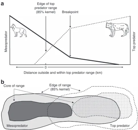
extensive landscapes. We propose the Enemy Constraint
Hypothesis (ECH), which predicts relatively weak top-down
control of mesopredators on the edge of top predator ranges, a
progressive decline in mesopredator abundance with increasing
distance into the core of top predator ranges, and mesopredator
numbers approaching zero where top predator abundance is at a
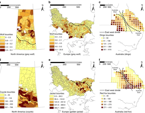
peak (Fig. 1). We tested the ECH by analysing bounty data from
North America (Saskatchewan), Europe (Bulgaria/Serbia) and
two regions from Australia in the State of Queensland (referred to
as Australia East and Australia West). Predator distributions in
these study areas provide opportunities to explore theoretical
questions under a natural experimental framework
13. In North
America and Europe, grey wolves
Canis lupus
(top predator) were
extirpated by humans from parts of their historical range,
resulting in the formation of new range boundaries (Fig. 2).
A similar process occurred for the dingo
Canis dingo
(top
predator) in Australia (Fig. 2). We used the existence of these new
range
boundaries
to
quantify
changes
in
mesopredator
abundance on either side of the range edge. The mesopredators
include the coyote
Canis latrans
(North America), golden jackal
Canis aureus
(Europe) and red fox
Vulpes vulpes
(Australia).
Our results, consistent across three continents, suggest that top
predators can suppress mesopredators to the point of complete
exclusion, but only when top predators occur at high densities
over large areas. The results suggest further that these conditions
are more likely to occur at the core than on the margins of top
predator ranges, providing support for the ECH. The results have
important implications for understanding species interactions
and niches, as well as the ecological role of top predators. More
broadly, there is a need to determine the causal mechanisms that
drive the observed trends (for example, predation, competition or
a mixture of both), and whether the results of the ECH apply to
other predator dyads that strongly interact and compete for
similar resources, or even to any strongly interacting competitive
species dyads (which we term ‘enemies’, Fig. 1).
Results
Indices of abundance
. The range limits for the species considered
in the study are shown in Figs 2 and 3. As expected, indices of
abundance based on bounty returns for each top predator were
low on the edge of its range and increased towards its range core
(Figs 3 and 4). Mesopredator abundance indices were higher
outside the current ranges of top predators and declined
pro-gressively with distance from the edge into each top predator’s
range (Figs 3 and 4).
Breakpoints
. In North America, Europe and Australia West,
abundance indices of mesopredators were close to zero within
each top predator’s range as indicated by breakpoints at 384,
214 and 320 km from the range edge, respectively (Fig. 4,
Supplementary Table 1,2). Breakpoints in the abundance indices
of top predators in North America, Europe, Australia West and
Australia East occurred at 241, 208, 259 and 302 km from the
range edge, respectively (Fig. 4, Supplementary Table 1,2). There
was no clear breakpoint where mesopredator abundance indices
in Australia East were close to zero, although the shape of the plot
was similar to all other sites (Fig. 4, Supplementary Table 1,2).
Edge of top predator range
(85% kernel) Breakpoint
a
b
Distance outside and within top predator range (km)
Core of range
Mesopredator Top predator
Edge of range (85% kernel) 0
[image:2.595.306.548.50.278.2]Mesopredator Top predator
Spatial correlation
. In North America (both species), Australia
East (both species) and Australia West (top predator) there was
no major spatial correlation based on plots of residuals versus
their spatial co-ordinates (Supplementary Figs 1,2,5,6,7), as
indicated by the lack of a pattern whereby groups of positive or
negative residuals are spatially clumped close to each other
17. In
Europe (both species) and Australia West (mesopredator) there
was minor clumping of the positive and negative residuals,
although not in any particular direction (Supplementary
Figs 3,4,8).
Discussion
The observed declines in indices of mesopredator abundance
could have been due to environmental gradients
15, land use
changes
18or other abiotic stressors
3that made conditions
progressively less suitable for each mesopredator. However, the
mesopredators we studied are habitat generalists; the coyote
occurs in a range of environments including urban areas and as
far north as Alaska
7, while the golden jackal occurs as far north as
Estonia and as far west as Switzerland
19. Accordingly, the
environmental conditions within the core ranges of our focal top
predators are suitable for these mesopredators, leading us to
expect that they would have occupied larger areas in the absence
of the top predator. Furthermore, we observed similar patterns of
abundance indices of the red fox in two distinctly different
physical environments. Australia West is predominantly arid,
whereas Australia East is more productive and contains
structurally complex forest areas. Yet, in both cases abundance
indices of red foxes declined progressively within the range of the
dingo.
An alternative explanation is that top predators exert negative
effects on mesopredators at all densities throughout their ranges,
but mesopredator numbers dwindle from the edge to the centre of
the top predator range because they are progressively cut off from
their larger source populations. This scenario would represent a
‘rescue effect’
20, by which small and isolated mesopredator
populations deep within the ranges of top predators are prevented
from going extinct by continuing inputs of immigrants. However,
mesopredator abundance indices declined close to zero within top
predator’s ranges in all cases assessed, therefore showing that
any immigration, progressively, became ineffective (Fig. 4). Thus,
while the ‘rescue effect’ may have contributed to the large
distances that mesopredators occurred within the ranges of top
predators, no mesopredator is likely to show such large
movements or range sizes that it would fully explain the
4200 km breakpoints.
The use of bounty data could have confounded the results if the
number of predators killed was influenced by (i) bounty price/
human effort, (ii) background fluctuations in populations or
(iii) poor weather for trapping and hunting. However, the same
bounty price was paid for a given predator in each hunting unit,
so bounty prices are unlikely to have driven changes in human
effort so as to produce the spatial gradients in bounty returns that
we observed. All the other factors apply equally to top predators
and mesopredators because of their biological similarities, so they
also are not likely to have driven the observed spatial patterns.
The bounty data we used are from published studies
7,13,16, and
bounty data are commonly used to derive indices of predator
abundance at large spatial scales
15. We are therefore confident
that the bounty data reflect spatial variation in predator
abundances. This argument is strengthened by the consistent
results we found across three separate continents, all of which
have different abiotic stressors, using different predator pairs.
Furthermore, despite the bounty data from Australia being
collected much earlier (1950s) in comparison to that in North
America (1982–2011) and Europe (2000–2009), the results in
Australia are corroborated by more recent evidence showing that
dingoes can suppress red fox populations
21.
In the absence of other available data, we suggest that top
predators progressively exert more top-down pressure the more
abundant they become towards the core of their ranges, such that
mesopredators disappear when deaths (induced by top predator
competition or killing) exceed births. The spatial gradient across
the range edge of the top predators that we examined is
essentially a surrogate for top predator abundance. Although not
essential for supporting the ECH, the existence of breakpoints in
the fitted lines for mesopredators and top predators may identify
abundance thresholds at which the top predator becomes
ecologically effective
22at suppressing the mesopredator, or the
key threshold beyond which the ecological effectiveness of the top
predator increases rapidly (Fig. 4). By implication, relationships
between top predators and mesopredators at large spatial
scales are frequency dependent
23, with top predators exerting
0 1,000 2,000 N N N
km
0 250 500
km
0 1,000 2,000
km
North America
Coyote
Grey wolf
Europe
Jackal
Grey wolf
Australia
Red fox
Dingo
a
b
c
Red fox
[image:3.595.54.540.50.238.2]Coyote Grey wolf Jackal Grey wolf Dingo
Figure 2 | Predator distribution during the study periods in each continent.Distribution is shown for (a) coyotes (hashed) and grey wolves (orange) in North America (Saskatchewan)7, (b) golden jackals (hashed) and grey wolves (orange) in Europe (Bulgaria and Serbia)16,19,27and (c) red foxes (hashed) and dingoes (orange) in Australia (Queensland)13,21. Note that the scales differ between continents. The black outline with dot in the centre denotes the
disproportionately higher levels of mesopredator suppression as
their abundance increases.
Our analysis supports historical accounts linking the rapid
expansion of mesopredator populations to the extirpation of top
predators
24, and suggests further that top predators can suppress
mesopredator populations, even to the point of complete
exclusion, as demonstrated in smaller scale studies
25. However,
the mere presence of a top predator may not be sufficient to exert
strong suppressive effects on mesopredators. This observation
could explain why some studies have documented only weak
effects of top predators on mesopredators
26. Furthermore, the
mesopredator breakpoints identified in North America and
Australia West were 143 and 61 km away from the top
predator breakpoints respectively. Both these mesopredator
breakpoints occurred well into each top predator’s range
suggesting there are expansive areas where these predators
coexist (Fig. 4). In Europe and Australia East the top predator
abundance indices also decreased at distances well away from the
range edge (Fig. 4). These decreases did not correspond with an
increase in mesopredator abundance indices in either case,
indicating the presence of abiotic stressors or that the habitats are
not well suited for either species. In the case of the latter, the
bounty data suggest that both grey wolves and golden jackals are
virtually absent from northern Serbia where there is intensive
agriculture, a finding that supports other studies
27,28. Similarly,
Eastern Australia (especially along the coastline) is a heavily
human-modified system in comparison to inland Australia, and
so this may explain the decline in dingo abundance indices that
we found on the far eastern side there.
Another factor that could limit top-down suppression of
mesopredators is that the social stability of top predators is often
altered by anthropogenic control
29,30, such that human influences
dampen the strength of top-down forcing
31,32and lead to a shift
in ecological state to a bottom-up driven system with increased
mesopredators
31. In our case studies, the ranges of top predators
contracted due to killing by humans and human modifications to
the environment (for example, habitat loss and fragmentation).
When assessing the ability of top predators to suppress
mesopredators, it may therefore be necessary to consider social
stability of top predators and other anthropogenically driven
influences on landscapes and foodwebs
18. Such investigations
would help to ascertain the circumstances where top predators
and mesopredators coexist, or where suppression occurs versus
complete exclusion. When considering grey wolves and coyotes,
0 250
a
b
c
d
e
f
Wolf bounties
0 – 0.5
0.6 – 1.7
1.8 – 3.2
3.3 – 5.5
5.6 – 9.4
0 – 40
41 – 144
145 – 233
234 – 350
351 – 766
0.0 – 39.3
39.4 – 124.8
124.9 – 231.8
231.9 – 369.6
369.7 – 648.1 0.0 – 0.5
0.6 – 2.1
2.2 – 4.5
4.6 – 9.3
9.4 – 20.6
0 – 50
51 – 130
131 – 210
211 – 350
351 – 615
0 – 35
36 – 100
101 – 180
181 – 270
271 – 410
North America (grey wolf) Europe (grey wolf) Australia (dingo)
North America (coyote) Europe (golden jackal) Australia (red fox)
Coyote bounties
Jackal bounties Wolf bounties
Dingo bounties
Red fox bounties East west divide
East west divide
Australia East Australia
West
Australia East Australia
West
500 N
N N
N N
N km
0 250 500
km
0 250 500
km
0 250 500km
0 250 500 km
[image:4.595.58.542.49.425.2]0 250 500km
complete mesopredator exclusion is possible, at least at historical
levels of top predator abundance across large landscapes
24. Even
more recently, complete exclusion has been found in relatively
closed systems (for example, Isle Royale National Park, USA
25),
although coexistence has been found in more open systems
where constant immigration by the mesopredators is possible
(for example, Riding Mountain National Park, Canada
33). Our
case studies suggest there is a point where mesopredators are
virtually absent well within top predator ranges, but it is not
possible to determine if this reflects complete exclusion or simply
low detection based on bounty returns.
The general predictions of the ECH can be tested for other
predator dyads that strongly interact and compete for similar
resources, and our predictions may be extended even further to
any strongly interacting competitive species dyads including
relationships involving parasites or pathogens (Fig. 1). In our
focal systems, the distance at which edge effects became manifest
was
4200 km (Fig. 4), but this distance will vary with other
species and ecosystem contexts. The ECH may yield insights
about early and cryptic impacts of landscape modification on
top-down forcing. Indeed, conservation efforts are often initiated
when species are close to extinction, rather than early on when
their populations are in the initial stages of decline. However, by
this stage the knock-on effects (for example, mesopredator
release
12) may have already taken place, with unknown effects on
ecosystem structure and biodiversity. If there is an imperative
to restore top predators, or any species that can induce
cascading effects that benefit ecosystems, then we need a better
understanding of the abundance and spatial extent at which these
species need to occur to perform their functional ecological roles.
Our analysis indicates that studies assessing the strength of
top-down mesopredator control will need to consider whether the
5
a
b
c
d
e
f
g
h
–0.32
–0.36
Wolf
Wolf
Dingo
Dingo
–0.40
–0.20
–0.30
–0.40
3
6
4
2
0 2
1
0 2.5
1.5
0.5
–0.5
1.5
0.5
–0.5
Mesopredator North America
Europe
Australia East
Australia West Australia West
Australia East Europe Top predator North America
4
3
Coyote 2 1
0
4
3
Jackal
Fox
Fox
2
1
0
–200 0 200 400 600 800
–200 0 200 400 600 800
–200 0 200 400 600 800
–200 0 200 400 600 800
Distance (km)
–200 0 200 400 600 800
–200 0 200 400 600 800
–200 0 200 400 600 800
–200 0 200 400 600 800
R2 = 0.38#
R2 = 0.3#
R2 = 0.5
R2 = 0.67#
R2 = 0.07#
R2 = 0.56#
[image:5.595.103.500.45.468.2]R2 = 0.64# R2 = 0.24#
mesopredator is located on the periphery or core of the top
predator’s range, and whether the top predator has reduced
abundance, destabilized social structure or a sporadic distribution
due to some external factor or factors. In the absence of such
considerations we may underestimate the potential effects of top
predators on ecological communities, thereby inhibiting top
predator conservation and restoration efforts.
Methods
Background
.
Predators are controlled by humans in many parts of the world. Where governments pay hunters a bounty for predator furs or scalps it is common practice to record the location (for example, hunting unit) where the predator was killed, and records are usually collated on an annual basis. Here, we collated bounty data from North America, Europe and Australia where mesopredators occur over large areas that also feature a gradient in top predator abundance. The data collection dates vary, and reflect the availability of bounty records for each continent. We used these datasets to test our hypotheses related to top predator and mesopredator distributions and abundances. Bounty data have been used in many previous studies to derive indices of top predator and mesopredator abun-dances7,15,34, based on the notion that predator abundance generally correlatespositively with the number of bounty returns7, and that bounty data can be used to
compare the abundances of top predators and mesopredators because of their biological similarities7. No other complementary predator abundance data exist at the spatial scales required.
North America
.
We retrieved bounty data on the number of grey wolves (top predator) and coyotes (mesopredator) killed in 136 hunting units in the province of Saskatchewan (651,900 km2), Canada, between 1982 and 2011. These data were collected by the Government of Saskatchewan each year based on payments made to trappers and hunters (Supplementary Table 3). The hunting units are also referred to as wildlife management zones, and these remained constant over the study period. Over the last two centuries, widespread predator control has resulted in grey wolves being largely restricted to northern forested areas in Saskatchewan, whereas they were, and continue to be, largely absent in the agricultural and rangeland areas to the south7. Coyotes were restricted to central North America in the 1800s, but had dispersed as far north as Alaska by the 1930s (ref. 7). Thus, by the beginning of our sampling, coyotes were present in Saskatchewan, including in areas with and without grey wolves (Fig. 2). Previous analyses of bounty data from Saskatchewan suggest that coyotes can disperse large distances (4200 km) into the northern forested areas where grey wolves occur7. Inthe previous analyses a coyote-to-red fox ratio was used to explore changes in the ratio of the two species on either side of grey wolf range. However, the range of the grey wolf was based on historical maps rather than bounty data, and there was no concurrent analysis of the grey wolf and coyote bounty data like that proposed herein.
Europe
.
We retrieved bounty data based on the number of grey wolves (top predator) and golden jackals (mesopredator) killed in 255 hunting units in Bulgaria (110,994 km2) between 2004 and 2009, and in 148 hunting units inneighbouring Serbia (88,361 km2) between 2000 and 2008. These data were
col-lected by the respective hunting associations in each county (Supplementary Table 3). Grey wolves were sporadically distributed or largely absent in these two countries in the 1970s, but they have since increased in numbers and dispersed into eastern Serbia and Bulgaria16,27. Golden jackals were restricted to two isolated populations in Bulgaria in the 1960s, but they now occupy northern and southern Bulgaria and at least in small numbers across large parts of Serbia16,19. Thus, by the
beginning of our sampling, golden jackals were present in Bulgaria and Serbia, including in areas with and without grey wolves (Fig. 2). Previous analyses of grey wolf and golden jackal bounty data from Bulgaria and Serbia suggest there is an inverse relationship between the abundances of the two species16. However, the full
extent to which golden jackals spatially overlap in distribution with grey wolves has not been assessed previously.
Australia
.
We retrieved bounty data on the number of dingoes (top predator) and red foxes (mesopredator) killed in the southern two thirds of Queensland, Australia (1,200,000 km2) between 1951 and 1952. These data were obtained from two mapspublished by the Queensland Government reporting the number of dingo or red fox bounties paid. The maps included locations of bounty records for both species, with one dot representing five dingoes or five red foxes. To allow for a spatial analysis and comparison of bounty records between the two species over the same area, the number of bounties paid for each species within a 100100 km area was used, following previously established protocols13. This approach resulted in a
comparison of bounty data over 145 defined locations across the study area. Dingoes were introduced into AustraliaB4,500 years ago, and at the time of European settlement (1788) they occupied the entire State of Queensland13,21.
However, by the 1950s (following a period of intensive control), dingoes were largely absent from central Queensland in sheep grazing areas. Red foxes were
introduced into Australia following European settlement and dispersed northward from southern Australia, eventually colonizing the southern two thirds of Queensland by the 1930s. Thus, by the beginning of our sampling, red foxes were present in Queensland, including in areas with and without dingoes (Fig. 2). As with the data from Europe, an inverse relationship between the abundances of dingoes and red foxes has been found in Queensland13. However, the full extent to
which red foxes spatially overlap in distribution with dingoes has not been assessed previously.
Patterns of spatial overlap
.
To assess patterns of spatial overlap between the top predator and mesopredator on each continent, we first mapped the number of predator bounties retrieved from each hunting unit in Arc GIS v10.1 (Environmental Systems Research Institute Inc.: Redlands, CA, USA). To stan-dardize the data we divided the total number of bounties by the number of years of data collection. We then characterized the distribution of the top predator in each continent by calculating a kernel density estimate from the mapped bounty data described above. For North America and Europe we used the entire mapped datasets, but because dingoes were virtually absent from the centre of the Aus-tralian study area (with two core areas of occupancy on either side) we split the data into two equal portions, one representing the eastern side, and the other the western side (Fig. 3). We chose the kernel density estimate because it provides a non-parametric method of estimating probability densities that is uninfluenced by effects of grid size and placement, and can accurately estimate the densities of any shape by superimposing a grid over the data and using information from the entire sample35. To calculate kernel densities, we converted the bounty data in eachcontinent into a point file using conversion tools in ArcView v10.1, with each point given the coordinates of the centroid of each hunting unit. We then used the kernel density estimator in the Geospatial Modelling Environment36package to create the
kernel density grid for each top predator dataset. This tool calculates kernel density estimates based on a set of input points and in this case we used the converted bounty data. The cell size for the kernel density estimate was standardized across all continents by setting the grid size at the scale of 2.5 km2.5 km. We used the default Gaussian (bivariate normal) kernel with the smoothed cross validation method to determine the level of smoothing because this approach does not typically overestimate space use37.
From the kernel density grid we calculated 85% probability contours for each top predator using the isopleth command in the Geospatial Modelling Environment package. The isopleth command creates a line based on a raster dataset representing a probability surface (that is, the kernel density estimate). Isopleths represent the boundary lines that contain a specified volume of a surface. For instance, the 0.95 isopleth represents the contour line containing 95% of the volume of the surface36. We used the 85% contour to define the edge of each top
predator’s distribution and used this edge as a proxy for a range boundary. The 85% contour was considered appropriate because it excluded outliers, and probability contours above 90% provided a gross overestimate of the top predator ranges based on the known distributional limits of each species (Fig. 2). Then, to assess top predator and mesopredator distributions and abundances across the study areas, we calculated the distance (km) from the centroid of each hunting unit to the closest point along the top predator’s 85% probability contour edge. We set the edge as the side of the circle where top predator densities were declining (that is, the edge of the range). Because we calculated distance from both sides of the contour edge, we multiplied the distance values from bounty units on the outside of the probability contour edge by 1. This step allowed the top predator and mesopredator data to be plotted along a continuous axis covering hunting units within and outside the top predator’s probability contour edge. Thus, distance valueso0 related to bounty units outside the contour edge and those40 represented bounty units inside the contour edge.
Predator abundance and distribution patterns
.
We used a piecewise linear regression to model the relationship between the top predator and mesopredator bounty data and distance to the edge of top predators range using the software R in the package siZer 0.1-4 (ref. 38) (Supplementary Methods). The piecewise linear regression allows multiple linear models to be fitted, and where the lines meet can be used to identify breakpoints where the slope of the linear function changes. Thus, the piecewise regression was chosen to determine if there are different linear trends over different regions of the data that accrued at a breakpoint, or in other words a sudden, sharp changes in slope of the line. We used the piecewise regressions, with one breakpoint that could occur at any predator bounty value. For the analysis, we excluded data from hunting units where there were no top pre-dators and no mesoprepre-dators. The bounty values were also standardized by sub-tracting the mean and dividing by the s.d. (z-scores) to allow for direct comparison among continents. Although not necessary for the ECH to hold (Fig. 1), we expected the sharp change in the mesopredator bounty data to occur where their abundance was close to zero. For the top predator we expected the sharp change to occur where their abundance starts to decline on the edge of the range. To estimateData availability
.
Data for Figs 3 and 4 are available from the Dryad Digital Repository http://dx.doi.org/10.5061/dryad.h1m85. Raw data are available from the first author upon request. R code is provided in Supplementary Methods.References
1. Elith, J. & Leathwick, J. R. Species distribution models: ecological explanation and prediction across space and time.Annu. Rev. Ecol. Evol. Syst.40,677–697 (2009).
2. Wiens, J. J. The niche, biogeography and species interactions.Philos. Trans. R. Soc. B Biol. Sci.366,2336–2350 (2011).
3. Louthan, A. M., Doak, D. F. & Angert, A. L. Where and when do species interactions set range limits?Trends Ecol. Evol.30,780–792 (2015). 4. Wisz, M. S.et al.The role of biotic interactions in shaping distributions and
realised assemblages of species: implications for species distribution modelling.
Biol. Rev.88,15–30 (2013).
5. HilleRisLambers, J., Harsch, M. A., Ettinger, A. K., Ford, K. R. & Theobald, E. J. How will biotic interactions influence climate change-induced range shifts?
Ann. N. Y. Acad. Sci.1297,112–125 (2013).
6. Estes, J. A.et al.Trophic downgrading of planet Earth.Science333,301–306 (2011).
7. Newsome, T. M. & Ripple, W. J. A continental scale trophic cascade from wolves through coyotes to foxes.J. Anim. Ecol.84,49–59 (2015).
8. Ritchie, E. G. & Johnson, C. N. Predator interactions, mesopredator release and biodiversity conservation.Ecol. Lett.12,982–998 (2009).
9. Caughley, G., Grice, D., Barker, R. & Brown, B. The edge of the range.J. Anim. Ecol.57,771–785 (1988).
10. Brown, J. H., Mehlman, D. W. & Stevens, G. C. Spatial variation in abundance.
Ecology76,2028–2043 (1995).
11. Ripple, W. J.et al.Status and ecological effects of the world’s largest carnivores.
Science343,1241484 (2014).
12. Crooks, K. R. & Soule´, M. E. Mesopredator release and avifaunal extinctions in a fragmented system.Nature400,563–566 (1999).
13. Letnic, M.et al.Does a top predator suppress the abundance of an invasive mesopredator at a continental scale?Glob. Ecol. Biogeogr.20,343–353 (2011). 14. Pasanen-Mortensen, M., Pyyko¨nen, M. & Elmhagen, B. Where lynx prevail,
foxes will fail - limitation of a mesopredator in Eurasia.Glob. Ecol. Biogeogr.22,
868–877 (2013).
15. Elmhagen, B. & Rushton, S. P. Trophic control of mesopredators in terrestrial ecosystems: top-down or bottom-up?Ecol. Lett.10,197–206 (2007). 16. Krofel, M., Giannatos, G., Cirovic, D., Stoyanov, S. & Newsome, T. M. Golden
jackal expansion in Europe: a case of mesopredator release triggered by continent-wide wolf persecution?Hystrix Ital. J. Mammal.http://dx.doi.org/ 10.4404/hystrix-28.1-11819 (2017).
17. Zuur, A. F., Ieno, E. N., Walker, N. J., Saveliev, A. A. & Smith, G. M. inMixed Effects Models and Extensions in Ecology with R(eds Gail, M.et al.) 161–191 (Springer, 2009).
18. Dorresteijn, I.et al.Incorporating anthropogenic effects into trophic ecology: predator–prey interactions in a human-dominated landscape.Proc. R. Soc. B Biol. Sci.282,20151602 (2015).
19. Trouwborst, A., Krofel, M. & Linnell, J. D. C. Legal implications of range expansions in a terrestrial carnivore: the case of the golden jackal (Canis aureus) in Europe.Biodivers. Conserv.24,2593–2610 (2015). 20. Brown, J. H. & Kodric-Brown, A. Turnover rates in insular biogeography: effect
of immigration on extinction.Ecology58,445–449 (1977).
21. Letnic, M., Ritchie, E. G. & Dickman, C. R. Top predators as biodiversity regulators: the dingoCanis lupus dingoas a case study.Biol. Rev.87,390–413 (2012). 22. Soule´, M. E., Estes, J. A., Berger, J. & Martinez del Rio, C. Ecological
effectiveness: conservation goals for interactive species.Conserv. Biol.17,
1238–1250 (2003).
23. Greenwood, J. J. D. & Elton, R. A. Analysing experiments on frequency-dependent selection by predators.J. Anim. Ecol.48,721–737 (1979). 24. Prugh, L. R.et al.The rise of the mesopredator.BioScience59,779–791 (2009). 25. Peterson, R. O. inEcology and Conservation of Wolves in a Changing World
(eds Carbyn, L. N.et al.) (Canadian Circumpolar Institute, University of Alberta, 1995).
26. Allen, B. L., Allen, L. R., Engeman, R. M. & Leung, L. K. P. Intraguild relationships between sympatric predators exposed to lethal control: predator manipulation experiments.Front. Zool.10,39 (2013).
27. Chapron, G.et al.Recovery of large carnivores in Europe’s modern human-dominated landscapes.Science346,1518–1519 (2014).
28. Sˇa´lek, M.et al.Population densities and habitat use of the golden jackal (Canis aureus) in farmlands across the Balkan Peninsula.Eur. J. Wildl. Res.60,
193–200 (2014).
29. Wallach, A. D., Ritchie, E. G., Read, J. & O’Neill, A. J. More than mere numbers: the impact of lethal control on the social stability of a top-order predator.PLoS ONE4,e6861 (2009).
30. Rutledge, L. Y.et al.Protection from harvesting restores the natural social structure of eastern wolf packs.Biol. Conserv.143,332–339 (2010). 31. Muhly, T. B.et al.Humans strengthen bottom-up effects and weaken trophic
cascades in a terrestrial food web.PLoS ONE8,e64311 (2013).
32. Worm, B. & Paine, R. T. Humans as a hyperkeystone species.Trends Ecol. Evol. 31,600–607 (2016).
33. Paquet, P. C. Winter spatial relationships of wolves and coyotes in riding Mountain National Park, Manitoba.J. Mammal.72,397–401 (1991). 34. Levi, T. & Wilmers, C. C. Wolves-coyotes-foxes: a cascade among carnivores.
Ecology93,921–929 (2012).
35. Seaman, D. E. & Powell, R. A. An evaluation of the accuracy of kernel density estimators for home range analysis.Ecology77,2075–2085 (1996).
36. Beyer, H. L.Geospatial Modelling Environment. http://www.spatialecology.com/ gme/ (2014).
37. Newsome, T. M., Ballard, G.-A., Dickman, C. R., Fleming, P. J. S. & van de Ven, R. Home range, activity and sociality of a top predator, the dingo: a test of the resource dispersion hypothesis.Ecography36,914–925 (2013).
38. Sonderegger, D.Package ‘SiZer’https://cran.r-project.org/web/packages/SiZer/ (2011).
Acknowledgements
We thank the Government of Saskatchewan in Canada, the National Hunting Association—Union of Hunters and Anglers in Bulgaria and the Executive Forestry Agency for providing hunting statistics data. The study was supported by the Ministry of Education, Science and Technological Development of Serbia (TR 31009).
Author contributions
T.M.N. conceived the study. T.M.N. and A.C.G. performed the data analysis. T.M.N. drafted the manuscript. All authors discussed the results and provided comments on the manuscript.
Additional information
Supplementary Informationaccompanies this paper at http://www.nature.com/ naturecommunications
Competing interests:The authors declare no competing financial interests.
Reprints and permissioninformation is available online at http://npg.nature.com/ reprintsandpermissions/
How to cite this article:Newsome, T. M.et al.Top predators constrain mesopredator distributions.Nat. Commun.8,15469 doi: 10.1038/ncomms15469 (2017).
Publisher’s note:Springer Nature remains neutral with regard to jurisdictional claims in published maps and institutional affiliations.
This work is licensed under a Creative Commons Attribution 4.0 International License. The images or other third party material in this article are included in the article’s Creative Commons license, unless indicated otherwise in the credit line; if the material is not included under the Creative Commons license, users will need to obtain permission from the license holder to reproduce the material. To view a copy of this license, visit http://creativecommons.org/licenses/by/4.0/