The dimensionality of niche space allows bounded and unbounded processes to jointly influence diversification

(1)

The dimensionality of niche space allows bounded

and unbounded processes to jointly in

ﬂ

uence

diversi

ﬁ

cation

Matthew J. Larcombe

1 , Gregory J. Jordan

2 , David Bryant

3 & Steven I. Higgins

1,4

There are two prominent and competing hypotheses that disagree about the effect of

competition on diversi

ﬁ

cation processes. The

ﬁ

rst, the bounded hypothesis, suggests that

species diversity is limited (bounded) by competition between species for

ﬁ

nite ecological

niche space. The second, the unbounded hypothesis, proposes that innovations associated

with evolution render competition unimportant over macroevolutionary timescales. Here we

use phylogenetically structured niche modelling to show that processes consistent with both

of these diversi

ﬁ

cation models drive species accumulation in conifers. In agreement with the

bounded hypothesis, niche competition constrained diversi

ﬁ

cation, and in line with the

unbounded hypothesis, niche evolution and partitioning promoted diversi

ﬁ

cation. We then

analyse niche traits to show that these diversi

ﬁ

cation enhancing and inhibiting processes can

occur simultaneously on different niche dimensions. Together these results suggest a new

hypothesis for lineage diversi

ﬁ

cation based on the multi-dimensional nature of ecological

niches that can accommodate both bounded and unbounded evolutionary processes.

DOI: 10.1038/s41467-018-06732-x

OPEN

1_{Department of Botany, University of Otago, PO Box 56, Dunedin 9054, New Zealand.}2_{Biological Sciences, University of Tasmania, Private Bag 55, Hobart,}

Tasmania 7001, Australia.3_{Department of Mathematics and Statistics, University of Otago, PO Box 56, Dunedin 9054, New Zealand.}4_{Plant Ecology,} University of Bayreuth, Universitätstraße 30, 95447 Bayreuth, Germany. Correspondence and requests for materials should be addressed to

M.J.L. (email:[email protected]) or to S.I.H. (email:[email protected])

123456789

(2)

S

pecies diversity has increased dramatically over geological

time

1

. Reconstructions using the fossil record are

ambig-uous about the causes of, and constraints on, this increase

2–4

_.

One important open question is whether the rate of species

accumulation slows as diversity increases, or is independent of

diversity

4–6

_{. The unbounded hypothesis implies that time, and}

the rate of evolution within clades (monophyletic branches of

phylogenies), control diversi

ﬁ

cation and that there is essentially

no limit on total diversity

3

_{. Alternatively, the bounded hypothesis}

suggests that diversity-dependent processes limit species

rich-ness

7

. This limit may be a true carrying capacity, or if extinction

is not zero, it is simply the equilibrium between speciation rate

and extinction rate

8

_{. Several mechanisms may cause}

diversity-dependent dynamics (see ref.

9

for a review), and the most widely

recognised of these involves competition for limited ecological

niche space

7

_{. Resolving this debate is essential for understanding}

limits to biodiversity, and why diversity is unevenly distributed in

space and time and between clades.

Previous attempts to discriminate between bounded and

unbounded diversi

ﬁ

cation have focused on modelling species

accumulation as inferred from phylogenies

10,11

and fossil

assemblages

5,6,12

_{, and to a lesser extent testing how ecological}

niche evolution impacts diversi

ﬁ

cation

13,14

. The results to date

have been inconclusive and often contradictory

2–4,15,16

,

indicat-ing that a more nuanced explanation may be required

4,16

_{. Here}

we quantify the extent to which both bounded and unbounded

processes in

ﬂ

uence species accumulation in the conifers. Our

analysis exploits methodological advances that allow us to infer

multi-dimensional physiological niche properties for large suites

of species

17,18

. We use these data to discriminate between the

distinctive niche characteristics predicted by the bounded and

unbounded hypotheses. Speci

ﬁ

cally we test support for the

bounded hypothesis

’

prediction that diversi

ﬁ

cation should slow as

niche overlap increases within clades

2,8

and the unbounded

hypothesis

’

prediction that niche evolution accommodates

increasing diversity by allowing the partitioning or expansion of

niche space

3,19,20

.

Conifers are an ecologically important, globally distributed

order of plants (Fig.

1 ; Supplementary Fig. 1) that are ideal for

this analysis. This large, well-studied lineage has well-de

ﬁ

ned

clades, excellent distribution data

21

_{, and is ancient enough (>300}

myo

22

_{) to assess how species accumulate through time. We use}

distribution data and a process-based species distribution model

(SDM) to infer physiological niche parameters for each of 455

living conifer species (75% of extant conifers). The niche

para-meters are combined with a robust fossil calibrated phylogeny

22

,

and interpreted statistically using a range of traditional

approa-ches including correlation analysis and rate through time plots, as

well as an a priori conceptual model of how niche and

phylo-genetic parameters relate to species richness. This conceptual

model postulates that species richness can be impacted both

directly and/or indirectly by clade age, multivariate niche

evolu-tion rate, and two novel metrics: clade niche size and the clade

competition index. Clade niche size is the projected potential

niche size (number of geographic grid cells occupied by all species

in the clade) corrected for clade species number (see Methods).

The clade competition index is the product of niche overlap and

geographic overlap between species within clades. The parameters

of the conceptual model were estimated using phylogenetically

constrained Bayesian path analysis. We conduct the analysis at

two phylogenetic levels, using 10 large clades and 42 smaller

clades. Our analysis shows that bounded and unbounded

diver-si

ﬁ

cation processes contribute more-or-less equally to diversi

ﬁ

-cation in conifers, and indicates that niche dimensionality may be

the mechanism by which these opposing forces work together.

Results and discussion

Quantifying diversi

ﬁ

cation processes

. We produced diversi

ﬁ

-cation rate through time plots for the full phylogeny and each of

the 10 large clades (Supplementary Fig. 2). This showed a range of

patterns including increases, slowdowns, long periods of stasis

and multiple rate changes, which is consistent with both bounded

and

unbound

processes

in

ﬂ

uencing

diversi

ﬁ

cation

in

conifers

9,23,24

_{. However, it has been shown that a number of}

factors may confound patterns of diversi

ﬁ

cation derived from

phylogenies in this way, and they are likely to be especially

problematic in old lineages with unobservable extinction

2,23,24

_.

Therefore given that conifers are an ancient lineage (>300 million

years old) that are believed to have been strongly in

ﬂ

uenced by

Cenozoic extinctions

25

_{, we pursued other forms of evidence to}

identify diversi

ﬁ

cation dynamics in this group.

To begin, we estimated the extent of correlations between

indices of diversi

ﬁ

cation, species competition, species richness

and niche size. These analyses suggest that both bounded and

unbounded processes in

ﬂ

uenced diversi

ﬁ

cation (Fig.

2 ). In line

with bounded diversi

ﬁ

cation, the clade competition index was

negatively related to species richness, and, as predicted by the

unbounded hypothesis, niche evolution was positively correlated

with species richness (Fig.

2 ). There was no clear relationship

between clade niche size and species richness, suggesting that

niche partitioning is an important diversi

ﬁ

cation process (Fig.

2 ).

That is, if speciation was largely occurring as a result of niche

expansion

—

where adaptation facilitates new species accessing

new ecological space

—

we would predict a positive relationship

between clade niche size and species richness because new species

expand the total clade niche size. Conversely, if speciation is

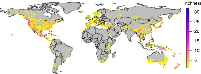
5 10 15 20 25 30 Species richness

Fig. 1Conifer species richness. Global species richness patterns in 455 conifer species based on cleaned empirical distribution data used here to analyse

[image:2.595.120.474.581.712.2]

(3)

occurring via specialization and the division of existing clade

niche space (i.e., niche partitioning) we would predict no

relationship between clade niche size and species richness because

adding new species does not expand total clade niche size. The

correlations further suggested a negative relationship between the

niche evolution rate and clade competition index. Unfortunately,

these simple correlation analyses cannot elucidate the relative

effects nor the role of indirect effects of the factors on clade

species richness. For these reasons we performed a

phylogeneti-cally constrained path analysis.

The path analyses revealed that diversi

ﬁ

cation in conifers was

in

ﬂ

uenced in almost equal measure by bounded and unbounded

processes (Fig.

3 ). In line with the bounded hypothesis,

competition with relatives (clade competition index) had a strong

negative effect on species richness, which suggests that available

niche space can limit species accumulation. This effect was strong

in both the 10 (

r

=

−

0.85) and 42 (

r

=

−

0.96) clade analyses.

Support for the unbounded hypothesis was evidenced by our

ﬁ

nding that niche evolution rate contributed positively to species

richness, suggesting that higher niche evolution rates within

clades allow more species to accumulate. This effect was stronger

in the 10 clade analysis (

r

=

0.61) than in the 42 clade analysis (

r

=

0.35). Furthermore, we found that clade niche size had neutral

(42 clade analysis) or negative (10 clade analysis) in

ﬂ

uence on

species richness, again suggesting that niche partitioning

constitutes the main mode of niche evolution in conifers. The

negative effect of clade niche size (10 clade analysis) is somewhat

counter-intuitive since it suggests that clades with smaller niche

volumes accommodate more species. However, this pattern is

consistent with niche partitioning accompanied by allee effects

and/or competition

8,26

driving random extinction processes that

lead to a reduction in clade niche size as postulated in Fig.

4 . In

fact the signi

ﬁ

cant direct effects of competition (

r

=

−

0.52) and

niche evolution (

r

=

−

0.19) on clade niche size, and relatively

strong negative effect of clade age (

r

=

−

0.21) on species richness

(Fig.

3 a), are consistent with such competition driven extinction

0.25 0.30 0.35 0.40 0.45 2.5

3.0 3.5 4.0 4.5

Clade competition index

Species richness

4 5 6 7 8 9 10 2.5

3.0 3.5 4.0 4.5

Niche evolution rate

Species richness

200 250 300 350 400 450 2.5

3.0 3.5 4.0 4.5

Niche size

Species richness

0.25 0.30 0.35 0.40 4

5 6 7 8

9

10

0.3 0.4 0.5 0.6 0.7 0.8 1.0

1.5 2.0 2.5 3.0 3.5

Species richness

0.0 0.5 1.0 1.5 2.0 2.5 1.0

1.5 2.0 2.5 3.0 3.5

Species richness

50 100 150 200 250 1.0

1.5 2.0 2.5 3.0 3.5

Niche size

Species richness

0.3 0.4 0.5 0.6 0.7 0.8 0.0

0.5 1.0 1.5 2.0 2.5

a

b

10 clade analysis

42 clade analysis

Fig. 2Associations between species richness and diversi_ﬁcation metrics. Scatter plots between clade species richness and selected clade metrics for two

divisions of the conifer phylogeny intoa10 large clades andb42 smaller clades. Straight lines indicate signiﬁcant linear effects detected using phylogenetic

generalized least squares (PGLS) regressions. The presence of multiple correlations made interpretation difﬁcult; for this reason, we performed a path

analysis (Fig.3)

–0.19 (0.06)

–0.88 (0.21)

0.61

–0.52 (0.06)

0.44 (0.18)

10 clade analysis (455 species)

42 clade analysis (429 species)

Parameters measuring bounded diversification

Parameters measuring unbounded diversification Clade niche

size

–0.88

Species richness

Clade age

–0.21

Clade competition

index

–0.85

–0.75 (0.22)

–0.99 (0.22)

–0.21 (0.16)

0.13 (0.08)

–0.03 (0.06)

0.35

0.15 (0.07)

0.35 (0.08)

Clade niche size

–0.03

Species richness

Clade age

–0.06

Clade competition

index

–0.96

–0.54 (0.11)

–0.77 (0.07)

–0.06 (0.07)

–

– –

–

+

– –

+

+/– The direction of significant effects (solid arrows) –

a

b

Fig. 3Path analysis of variation in conifer species richness. Bayesian path

analysis showing the relative effects of niche and phylogenetic parameters

on clade species richness for 455 conifer species ina10 large clades andb

42 smaller clades. Total effect size is shown in bold, while direct effects and their standard deviation are shown along the vertices. Solid lines indicate

[image:3.595.53.541.58.299.2] [image:3.595.308.547.371.642.2]

(4)

processes unfolding through time

8

. The lack of evidence for this

causal pathway in the 42 clade analysis probably re

ﬂ

ects the much

younger average clade age (17 my compared with 112 my), and

smaller clade sizes, which mean that partitioning and extinction

processes (Fig.

4 ) will be less frequent and therefore more dif

ﬁ

cult

to detect. This interpretation is consistent with previous work

suggesting extinction played a pivotal role in the diversi

ﬁ

cation of

conifer clades in the Cenozoic, while younger clades are primarily

shaped by recent speciation

25

_.

We note that our clade competition index under-estimates

competition because it may not capture all potential competitive

interactions. Our measure quanti

ﬁ

es expected competition

between members of a clade based on overlap in geographic

space and niche space (see Methods). It is an underestimate

because, although competition is likely to be most intense

between close relatives (i.e., members of the same clade),

competitive interactions with more distantly related species are

also likely and not captured by our metric

27–29

. Incorporating

competition with distantly related species, although possible,

would require additional data and necessitate additional

assump-tions. It is also possible that our clade competition index fails to

detect some forms of competition that might constrain

diversi

ﬁ

cation rates. For example, it is possible that competition

between ecologically similar species may prevent them from

becoming sympatric as has been reported in some bird

lineages

30,31

_{. Such processes could limit range expansion and}

potentially reduce diversi

ﬁ

cation rates if range expansion

increases the likelihood of diversi

ﬁ

cation

—

for example by

increasing the probability of allopatric speciation

9

_.

Although

much

work

has

favoured

either

bounded

2,10,14,28

or unbounded

3,32,33

processes driving diversi

ﬁ

-cation, our results are consistent with observational

12,19

_,

theoretical

16

_{and modelling}

4,12

_{work, which suggests that both}

bounded and unbounded processes in

ﬂ

uence diversi

ﬁ

cation. For

example, much of the empirical evidence is consistent with

diversi

ﬁ

cation slowing, rather than reaching an asymptote

16,19

_.

This led Cornell

16

to propose the

“

damped increase

”

hypothesis,

which in line with our results, suggests that competition induced

by niche

ﬁ

lling reduces diversi

ﬁ

cation rate, while specialisation or

new ecological opportunities counteract this effect

16

. Others have

extended these ideas to show that the incongruity between strict

bounded and unbounded views could be overcome by allowing

diversity-accumulation-models to vary between periods of either

bounded or unbounded diversi

ﬁ

cation

4

. These studies do not,

however, provide a population/species level mechanism that

could drive shifts in diversi

ﬁ

cation processes

4

.

Niche dimensionality and diversi

ﬁ

cation

. To address this

mechanistic basis, we examined whether niche dimensionality can

drive variation in diversi

ﬁ

cation processes

4,34

. We used a range of

statistical procedures to determine if variation exists in the

evolu-tionary

ﬂ

exibility of niche traits at three levels: (1) across the

phy-logeny; (2) within clades; and (3) between clades. Across the full

phylogeny we found variation in the level of conservatism

(phylo-genetic signal) between traits (with Pagel

’

s

λ

values ranging from

<0.01 to 0.42; Table

1 ), suggesting variation in the evolutionary

ﬂ

exibility of niche dimensions. This variation between traits was also

evident within clades, for example in Clade 7,

Pinus

(Table

2 ). In

fact, mixed effects modelling show that signi

ﬁ

cant variation exists in

evolutionary rate between traits after accounting for random

varia-tion between clades (

trait

:

F

10,90

=

62.5,

P

=

<0.0001), suggesting

that trait evolution rates do, on average, vary within clades.

We also found that the evolution rate of traits varies between

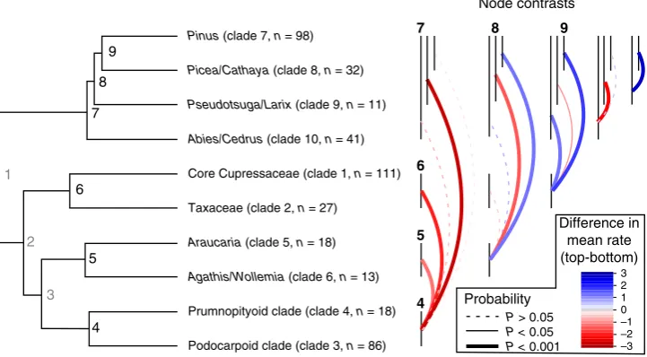
clades, for example, Fig.

5 summarises how the evolution rate of

traits varies across the clade-level phylogeny after accounting for

non-independence associated with phylogenetic relationships

(using phylogenetic independent contrasts

35

_{). This analysis}

indicates that trait evolution rate varies signi

ﬁ

cantly across the

terminal nodes of the clade-tree (node:

F

8,80

=

6.4,

p

< 0.0001).

Diversification via niche partitioning

Clade niche size

Time 1

n = 2

Time 2

n = 5

Present

n = 4 Extinction gap

Allee effects and/or competition drive extinction

Clade niche size = time 1 Clade niche size < time 1

Fig. 4Extinction driven reduction in clade niche size. Example of how niche

partitioning combined with extinction associated with allee effects and/or competition, can result in a negative relationship between clade niche size

and species richness as found in Fig.3a. Different coloured curves

[image:4.595.47.290.304.482.2]

represent species

Table 1 Phylogenetic signal across the full phylogeny

Niche trait λ P(λ) K P(K)

Soil moist N uptake (3) 0.144 <0.001 0.019 0.001

Max temp growth (4) 0.000 1 0.016 0.039

Min temp growth (3) 0.092 <0.001 0.016 0.115

Soil moist N uptake (2) 0.444 <0.001 0.023 0.001

Mean temp growth (2) 0.205 <0.001 0.020 0.001

Soil moist growth (2) 0.362 <0.001 0.021 0.001

Radiation growth (2) 0.054 0.064 0.018 0.005

Min temp growth (2) 0.415 <0.001 0.024 0.001

N soil growth (1) 0.158 <0.001 0.019 0.004

N soil growth (2) 0.132 <0.001 0.017 0.012

Mean temp N uptake (2) 0.215 <0.001 0.021 0.001

Phylogenetic signal in the 11 key niche traits based on a conifer phylogeny covering 455 species and estimated using Pagel’sλand Blomberg’s K. Thep-value (P) forλis estimated using the likelihood

ratio test. Thep-value for K is estimated from a randomization test based on 1000 simulations of the data. The numbers in parentheses indicate the position of the speciﬁc trait in the growth or resource

[image:4.595.45.550.565.702.2]

(5)

Looking at the terminal nodes is interesting because it provides

inference regarding the descendent clades, and Fig.

5 shows that

high rates of trait evolution are often associated with increases in

diversity, and vice versa. For example, nodes that give rise to

relatively high diversity clades (e.g., nodes 4, 7 and 9; Fig.

5 ) tend

to have have signi

ﬁ

cantly higher trait evolution rates than nodes

that give rise to lower diversity clades (i.e., nodes 5 and 8; Fig.

5 ).

The only exception to this pattern is node 6, which is parent to

the high diversity Clade 1 (

n

=

111), and has a relatively low trait

evolution rate (Fig.

5 ). Interestingly, Clade 1 also has the lowest

clade competition index of any clade in our analysis, possibly

suggesting that in the absence of strong competition, diversi

ﬁ

ca-tion has advanced without a parallel increase in trait evoluca-tionary

rates. Allopatric speciation in an ecologically specialised, and well

dispersed linage might explain this type of pattern. The most

diverse genus in Clade 1,

Juniperus

, is unusual among conifers in

its preference for relatively arid, warm climates and calcareous

soils, furthermore the evolution of

“

berry-like

”

fruits is thought

have driven extensive dispersal and allopatric speciation in the

genus

36

_{. Together, the above results imply that trait evolutionary}

rates vary within and between conifer clades, and in combination

with competitive interactions this variation can explain shifts in

clade-level diversity.

Such variation in the evolutionary

ﬂ

exibility of traits and

competition between species within clades may accommodate the

operation of both bounded and unbounded processes. This can be

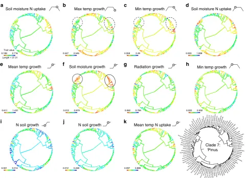
seen more clearly by focussing attention on single clades. For

example, in Clade 7 (

Pinus

, Fig.

6 ), the effect of soil moisture on

growth (Fig.

6 f) is highly conserved in the sub-clades highlighted

with solid ellipses, suggesting that interspeci

ﬁ

c competition is likely

to be high along this niche dimension in these sub-clades. However,

these same sub-clades are labile in terms of their temperature

requirements for growth (traits b and c, highlighted with dashed

ellipses in Fig.

6 b, c), indicating that evolution and specialisation are

possible along these niche dimensions (Fig.

6 ). Analogous patterns

[image:5.595.49.550.71.198.2]

can be seen in the other

Pinus

sub-clades (Fig.

6 ) and the other

Table 2 Phylogenetic signal within Clade 7 (

Pinus

)

Niche trait λ P(λ) K P(K)

Soil moist N uptake (3) 0.569 0.003 0.080 0.005

Max temp growth (4) 0.000 1.000 0.076 0.011

Min temp growth (3) 0.000 1.000 0.058 0.286

Soil moist N uptake (2) 0.623 0.026 0.097 0.001

Mean temp growth (2) 0.167 0.051 0.092 0.001

Soil moist growth (2) 0.609 0.033 0.079 0.003

Radiation growth (2) 0.000 1.000 0.079 0.005

Min temp growth (2) 0.104 0.208 0.072 0.015

N soil growth (1) 0.000 1.000 0.067 0.076

N soil growth (2) 0.000 1.000 0.062 0.159

Mean temp N uptake (2) 0.004 0.894 0.077 0.004

Phylogenetic signal in the phylogeny of 111 species ofPinusfor 11 key niche traits, estimated using Pagel’sλand Blomberg’s K. Thep-value (P) forλis estimated using the likelihood ratio test. Thep-value

for K is estimated from a randomization test based on 1000 simulations of the data. The numbers in parentheses are as Table1

Podocarpoid clade (clade 3, n = 86) Prumnopityoid clade (clade 4, n = 18) Agathis/Wollemia (clade 6, n = 13) Araucaria (clade 5, n = 18) Taxaceae (clade 2, n = 27)

Core Cupressaceae (clade 1, n = 111) Abies/Cedrus (clade 10, n = 41) Pseudotsuga/Larix (clade 9, n = 11) Picea/Cathaya (clade 8, n = 32) Pinus (clade 7, n = 98)

Difference in mean rate (top-bottom)

2 1

–1 –2 0 3

–3

P > 0.05

P < 0.001 P < 0.05

Probability

4 5 6

9

8

7

1

2

3

4 5 6

7 8 9

Node contrasts

Fig. 5Phylogenetic independent contrasts of niche evolution rate. Left: clade-level conifer phylogeny showing terminal nodes (4–9) in bold black, internal

nodes (1_–3) in grey (not consider in the contrasts). Taxonomic information about the groups, as well as their clade number and species richness (Clade #,

n=species richness) are given at the tips. Right: Contrasts between the terminal nodes. The vertical bars correspond to the terminal nodes (labelled once

in bold to match those on the tree), and the coloured arcs show the difference in mean niche evolution rate between the nodes (calculated by subtracting the mean of the top node from the mean of the bottom node). For example the red line joining nodes 5 and 4 indicates that the niche evolution rate at node

5 is 1.3 lower than node 4. Signiﬁcance is indicated by line thickness and type. The pattern that emerges is that the nodes which give rise to clades with high

species richness (e.g., nodes 4 and 9) have signiﬁcantly higher niche evolution rates than nodes giving rise to clades with low species richness (with the

[image:5.595.118.479.252.451.2]

(6)

clades (Supplementary Fig. 3). Population level studies investigating

how individual traits respond under direct interspeci

ﬁ

c competition

in actively diversifying linages are needed to help clarify how these

processes operate at the ecological level.

By considering the multi-dimensional nature of niche

evolu-tion, we have shown how bounded and unbounded diversi

ﬁ

cation

processes may simultaneously control diversi

ﬁ

cation rates. Niche

dimensionality has long been thought to promote diversity by

partitioning resources and facilitating coexistence

37

_{, and there is}

considerable empirical support for this hypothesis

34

_{. Most}

previous assessments of how niche characteristics impact

macro-diversi

ﬁ

cation have used low dimensional proxies of the

niche such as body size

14

_{or climatic range}

13

_{. In contrast, our}

assessment of multiple, physiological niche traits, reveals that

both diversity-limiting competition, and diversity-promoting

evolution may operate concurrently. At the population level

these processes are likely to be separated in space and/or time

—

in

line with models by McPeek

38

and Marshall and Quental

4

,

respectively. For example, populations along environmental

gradients could experience variation in the opportunity for

specialisation or niche expansion along some niche dimensions

but experience competition along other niche dimensions

38

_.

Similarly, changes in the environment could induce temporal

variation in selection pressure that affects the interplay between

conservative and labile niche traits

4

_.

In summary, we have identi

ﬁ

ed how processes that de

ﬁ

ne the

niche geometry of conifer clades can jointly promote and

constrain diversi

ﬁ

cation. Our results con

ﬁ

rm that the contrasting

processes that underpin bounded and unbounded diversi

ﬁ

cation

have both operated during the evolution of a major lineage. Our

study thereby provides an analysis framework for a new

multi-dimensional-niche hypothesis that uni

ﬁ

es the bounded and

unbounded hypotheses

4,12,16,19

.

Methods

Data acquisition and preparation. Geo-referenced collection data for all conifer

species were extracted from the Global Biodiversity Information Facility (www.gbif.

org). These data were supplemented by published species records not in GBIF

from39–44. Climate estimates were made for each point record, using Worldclim45_.

Data was cleaned manually byﬁrstly eliminating duplicate records, then for

con-sistency with species distribution descriptions39_{, and then by comparing}

World-clim estimates of altitude, with the altitudes provided with each site record. Where Worldclim altitudes were inconsistent with the altitude in species descriptions by more than 300 m, we replaced these records with estimates from nearby sites with altitudes consistent with the descriptions.

Estimating physiological niche traits. We estimated the physiological niche traits of the study species using a physiologically-based approach to species distribution

modelling17_{. This method uses the Thornley transport resistance (TTR) model of}

plant growth46_{to estimate the niche traits that match the observed distribution of}

species. The TTR model46_{, is an ordinary differential equation that models how}

plant growth is inﬂuenced by carbon uptake, nitrogen uptake, and the allocation of

0.189 2.716

Trait value

0.547 2.545 0.359 2.49 0.003 1.008

0.611 1.431 0.012 0.979 0.062 0.784 0.022 0.932

0.001 0.314 0.012 0.458 0.097 0.886

Pinus nelsonii

Pinus balfouriana Pinus longaeva Pinus aristata Pinus quad

rifolia

Pinus monoph ylla

Pinus maximar tinezii

Pinus pinceana

Pinus r zedowskii Pinus edulis Pinus culminicola

Pinus remota Pinus cembroides Pinus squamata

Pinus b ungeana Pin us ger ardiana Pin us krempfii Pin us peuce Pin us fle xilis Pin us ayacahuite Pin us strobi formis Pin us stro bu s Pin us monticola Pin us lamber tiana sil u a ci bl a s u ni P ar ol fi vr a p s u ni P Pi n us k o ra iensis Pin us w a llichiana Pi n us sibir ica Pi n us dalatensis Pi nus pumila Pi nus bhutanica Pi

nus fenz

eliana Pi

nus ar mandii Pi nus mor risonicola Pin us canar iensis Pi nus pinaster Pinu

s r_ox burghii Pi_{nus pinea} Pinu

s b_rutia Pi_{nus halepensis} Pin

us heldreichii Pinus me

rkusii Pinus resinosa

Pinus hw angshanensis Pinus massoniana Pinus tropicalis Pinus sylvestris Pinus densiflora Pinus nigra Pinus mugo Pinus uncinata Pinus taiwanensis

Pinus kesiya

Pinus densata

Pinus luchuensis

Pinus tab

uliformis

Pinus yunnanensis Pinus conto rta Pinus clausa

Pinus virginiana Pinus pseudostro bus

Pinus ha rtwegii

Pinus montezumaePin us ar izonica Pin us engelmannii Pin us d

evoniana Pin us jeffr eyi Pin us du rangensis Pin us coulte ri Pin us douglasianaPin

us torre yana Pin us sabiniana a s or e d n o p s u ni P at a u n et t a s u ni PPin us radiata Pin us m u ricata Pi n us patula Pi nus teocote

Pi nus leiop

hylla Pi

nus lumholtzii Pi

nus greggii Pi

nus cubensis Pin us la wsonii Pi nus p ringlei Pi_nu s ooca rpa Pi_nu s car ibaea Pi nus serotina Pin us rigida Pin us pungens PinPinus pr_{us taeda}aeter

missa Pinus glab ra Pinus herre rae Pinus palust ris Pinus echinataPinus occidentalis

Pinus elliottii

Length = 37.31

Radiation growth Soil moisture growth

Mean temp growth

Soil moisture N uptake Max temp growth Min temp growth

N soil growth

Soil moisture N uptake

Min temp growth

N soil growth

Clade 7: Pinus Mean temp N uptake

a

b

c

d

e

f

g

h

i

j

k

Fig. 6Niche dimensionality in_Pinus. Phylogenies of Clade 7 (_Pinus) showing ancestral state reconstructions of the 11 most important niche dimensions in

order of importance (a–k). The bottom right panel shows the same phylogeny with species names. Sub-clades withinPinuswith conservative (solid ellipse)

and labile (dashed ellipse) niche dimensions are highlighted and discussed in the text (see Results and Discussion). Theﬁlled circle on trapezoid and step

[image:6.595.57.541.46.395.2]

(7)

carbon and nitrogen between roots and shoots. It explicitly separates the physio-logical processes of resource uptake from biomass growth. The implementation by

Higgins et al.17_{relates the uptake and growth processes to environmental forcing}

variables. Speciﬁcally, the model considers how carbon uptake might be limited by temperature, soil moisture, solar radiation and shoot nitrogen; nitrogen uptake might be limited by temperature, soil moisture and soil nitrogen; and growth and

respiration loss might be inﬂuenced by temperature. The model runs on a monthly

time step, which allows it to explicitly consider how seasonalﬂuctuations in the

forcing variables interactively inﬂuence plant resource uptake and growth. Higgins

et al.17_{provides a full description of the model and its assumptions.}

We use the cleaned presence dataset described above to identify locations where the species occur. A variety of methods for simulating absence points (often called pseudoabsence points) are available, but the method adopted is regarded as a

relatively small source of error47_{. Our method balances the number of presence and}

absence points and stratiﬁes the selection of absence points by environment type.

To deﬁne environment types we use a partitioning algorithmclara48_{to classify the}

TTR environmental forcing variables into 25 environmental zones. We further restricted the selection of absence points to the zoological realm(s) where the species occurs and to distances >0.25 degrees from the presence points. This approach helps ensure that a representative range of environmental zones are included in the absence samples and that they are selected within a dispersal zone that is potentially reachable on an ecological time scale (i.e., the zoological realms). The model predicts the potential biomass of an individual plant as a function of

the environmental forcing variables at a site. Following the work of Higgins et al.17_,

we assume thatpi, the probability of a species occurring at sitei, is described by the

complementary loglog of the modelled plant biomass at siteiand that the

likelihood of observing the presence–absence data (yi) at siteiis described by the

Bernoulli distribution. To estimate the parameters, we used the differential

evolution optimization algorithm49_to_{ﬁnd the set of parameters that maximizes}

this likelihood over all sites. The modelﬁts were evaluated by examining the

confusion matrix (a matrix comparing the number of true positives, true negative, false positives and false negatives), with particular weight given to the false negative rate, i.e., instances where the model predicts the species to be absent, but it is actually present (Supplementary Data 1).

Like most species distribution modelling techniques, our analysis predicts the potential niche of a species. In most situations biotic interactions and dispersal limitations will prevent species occupying the full extent of their potential niche. With this in mind we restrict projection of potential species ranges to the subset of

environmental zones (see above) present in each species’occurrence data; this

prevents predictions beyond the data domain used for estimating the model parameters. We calculated the niche size of species in two ways: (1) projecting species ranges for the world, and (2) using a resampled dataset that assumes that the worlds environmental zones are equally common. This second method corrects for any bias in projected range size introduced by variation in the extent of different environmental zones, but maintains the covariance structure of the

environmental data50_{. To create a dataset where each environmental zone is}

equally common, we created a resampled dataset of the environmental data. We

again useclarato classify the global TTR input data into 50 environmental zones.

We then sampled aﬁnite number (1000 in our case) of locations from each of 50

environmental zones, which produces an environmental dataset where each environment zone is equally represented. We projected the range sizes of species in this resampled environmental space. Analyses conducted using geographic locations and resampled locations yielded very similar results. The analysis based on resampled locations is presented in the main manuscript while the analysis based on geographic locations is available in Supplementary Fig. 4.

Phylogenetic methods. We used the fossil calibrated conifer phylogeny of Leslie

et al.22_{, which is based on two chloroplast genes and two nuclear genes. We}

pruned this 487 species tree to match the 455 species for which we had good distributional data. Although a clade is any monophyletic group in a phylogeny, the ability to detect effects in clade-wise analysis will be in part reliant on having

enough variation in clade size51_{. Therefore we developed two clade classi}_ﬁ

ca-tions. Theﬁrst inclusive division is based on tree topology at deeper well

sup-ported nodes, and it aimed to retain major taxonomic groups such asPinus,

resulting in 10 clades (Supplementary Data 1). The second lower division is based on a time-slice approach at Eocene/Oligocene boundary (33.9 ma). Using the tree topology closer to the tips than this becomes more difﬁcult. This second approach produced 68 clades, 28 of which included a single species. These single species were dropped from the analysis, leaving 42 clades and 429 species in the second analysis (Supplementary Data 1). We recognize that removing single species clades might bias rate estimates because these are the clades with the

lowest diversiﬁcation. However, the dataset still covers a wide range of clade

species richness (2–45 species), and meaningful estimates for single species

cannot be calculated for most subsequent metrics used in our analysis (e.g., niche evolution rate, clade niche overlap, clade geographic overlap etc.). Furthermore, this potential bias only affects the 42 clade analysis and the general agreement between the 10 and 42 clade analyses (see Results and Discussion) suggests that any effect is inconsequential.

We produced diversiﬁcation rate through time plots using BAMM (Bayesian

analysis of macroevolutionary mixtures). BAMM was run on the full tree of

455 species with following parameter settings: the sampling fraction was set at 0.762; the priors were estimated from the tree using setBAMMpriors in

BAMMtools52_{in R, the expected number of shifts was one, the lambda initial prior}

was 12.414, the lambda shift prior was 0.003414, the mu initial prior was 12.414 and the lambda time variable prior was 1; MCMC was run for 2,000,000 generations, write frequency was 2000, print frequency was 100, and the acceptance rate was 10; all other settings were set to the BAMM defaults. Clade-level BAMM runs were done using clade-level phylogenies pruned from the full phylogeny, sampling fractions adjust to reﬂect exact clade coverage, and priors were adjusted

using setBAMMpriors. Rate through time plots with conﬁdence shading were

produced in BAMMtools for the full tree and each of the 10 clades separately (Supplementary Fig. 2).

Clade-level metrics. For each clade we calculate the following metrics: age; niche size (number of geographic grid cells occupied by all species in the clade) is the projected potential niche size; niche evolution rate; and clade competi-tion index. The crown age of the clade was calculated directly from the tree

using the branching time function in APE53,54_{. When assessing niche size, we}

needed to control for the number of species in the clade. In the 10 clade analysis, the smallest clade contained 12 species. Instead of using the direct niche size of each of a clade, we instead randomly subsampled subsets of 12 species from each clade, computing the niche size for each subsample, and taking the mean of these values. The resampling was repeated 10,000 times. In the 42 clade analysis we used the same procedure, except that subsamples of size 2 were used.

The calculation of niche evolution rate involves using a multivariate model. The TTR species distribution model estimates 24 parameters associated with plant

growth (see above). For this reason weﬁrst extracted the most informative of the 24

niche parameters for the analysis, speciﬁcally we used phylogenetically corrected

principal components analysis (PCA)55_{to identify which model parameters had}

the most inﬂuence on shaping niche space in our dataset. PC 1 to 8 explained over

94 percent of the variation in the dataset. The most inﬂuential parameters were

identiﬁed based on the eigenvector loadings >0.3, and vector plots were used to

exclude correlated parameters. This procedure identiﬁed 11 parameters (Figs5,6)

which were ranked in order of importance by summing the effect of each trait on each PC weighted by the proportion of the variance explained by that PC. For the

10 clade analysis, these 11 parameters wereﬁt together in a multivariate Brownian

motion (BM) model of evolution in OUCH56_{. In the 42 clade analysis, because}

some clades had only two species there were insufﬁcient degrees of freedom to use

a multivariate model, and a univariate Brownian motion (BM) model of evolution

wasﬁtted using the most important parameter (the effect of soil moisture on N

uptake3_{; see Figs}₅_,₆_{). Following}13_{, the trait evolution model was used to calculate}

the variance–covariance matrix for the traits in each clade. The diagonal elements

of this trait matrix represent the phylogenetic rate of character evolution which were summed to provide a multivariate (or univariate) rate parameter for each

clade—the niche evolution rate13_.

The bounded hypothesis proposes that competition plays a key role in limiting diversiﬁcation. Competition is likely to be most intense between close relatives due

to similar physiological requirements (or niches) wherever species co-occur8_{. To}

estimate competition, we produce a metric which summarises the degree of expected niche overlap and observed geographic overlap between species within

clades. Schoener’s index57_{of niche overlap was estimated for each pair of species}

from the projected species distributions (i.e., the potential niche of the species) in

SPAA58_{, and the subsequent matrix was rescaled so the values range between 0 and}

1. For each pair of species we computed the the average distance between each geo-referenced occurrence record for one species and each geo-geo-referenced occurrence record in the other. These values were also normalised over all pairs of species to produce a matrix of values between 0 and 1. We subtracted each value from 1 to

give measures of species overlap. The competition index for two species is deﬁned

to be the product of the niche overlap and the measure of geographic overlap. The

“clade competition index”for a clade is deﬁned as the average of the competition

indices between all species in the clade.

This formulation of the clade competition index ensures that, if species are randomly permuted, the expected value of the index for a clade is simply equal to the mean competition index between all pairs of species (by the linearity of expectation). Hence, the expected clade competition index is independent of clade size. We further veriﬁed the lack of bias by simulation. We randomly shufﬂed the species names at the tips of the phylogeny, to produce 10 clades of the same size as those in our analysis, but with a random compliment of species. We then calculated the clade competition index for each randomised clade as above and stored this result. This process was repeated 10,000 times. The average clade competition score (based on the 1000 replicates) was then plotted against species richness for comparison with the empirical data (see Supplementary Fig. 5). We used least squares regression to test the relationship between clade species richness and the randomised clade competition index, with the expectation that any bias in the

metric would result in a signiﬁcant deviation from zero.

(8)

Phylogenetic generalized least squares (PGLS) regression models were used to look for signiﬁcant correlations, with the clade competition index and niche evolution rate square root transformed to meet the assumptions of normality.

We developed an a priori conceptual model (Fig.3) to estimate the relative

effects of clade niche size, niche evolution rate, clade age and the clade competition

index on species richness. The unbounded model predicts that speciﬁc evolutionary

characteristics, controlled by phylogenetic niche conservatism, lead to clade-specific diversification rates. This has two consequences: (1) when the effect of diversification rate is factored out older clades will have more species than younger

clades; and (2) positive diversiﬁcation will involve niche evolution that manifests as

either the expansion or partitioning of clade niche space as species accumulate. In line with these predictions our model allows: (1) clade age to directly inﬂuence

species richness; and (2) niche evolution rate to inﬂuence species richness both

directly, and indirectly, via its effect on clade niche size, with the direct relationship between clade niche size and species richness indicating the mode of niche evolution (expansion or partitioning). Conversely, the bounded diversity model predicts that competition for limited resources places a limit on species number. It has long been recognised that competition is likely to be most intense between close relatives, because the ecological requirements of relatives are likely to be similar due

to phylogenetic niche conservatism. Our clade competition index quantiﬁes

competition between the species within a clade. Therefore we allow the clade competition index to directly effect species richness, however, because the clade

competition index quantiﬁes interactions between niches, it is also allowed to

indirectly inﬂuence species richness via its effect on the niche evolution rate, and clade niche size.

We used Bayesian path analysis to calculate the effects in the path diagram

(Fig.3), while accounting for non-independence associated with phylogenetic

relationships59_{. The total effect of each model parameter on the response variable}

(species richness) was calculated from the direct and indirect effects following

Schumacker and Lomax60_{. All model parameters were normalised and centred to a}

mean of zero and constant standard deviation. Following Rabosky et al.61_{, we use}

relative log-transformed species richness. For each analysis (10 and 42 clade), the full phylogenetic tree was collapsed to the clade level, and the inverse of the

variance–covariance matrix from this clade-tree was used to explicitly correct for

the phylogenetic dependencies between clades. Modelling was undertaken using

JAGS62_{running three chains for 15,000 iterations, after a burnin of 25,000, and}

thinning the chains to everyﬁfth sample. Normal uniformed priors we used for the

path effects. The package coda63_{was used to produce trace plots for diagnosing}

convergence.

Niche trait analysis. We used a phylogenetic trait analysis to quantify the evo-lution of individual niche dimensions at the level of the full phylogeny and within clades. This analysis focused on the 11 niche dimensions identiﬁed above.

Phylo-genetic signal across the full phylogeny and in detail for clade 7 (pinus), was

estimated using Pagel’sλ64_{, with signi}_ﬁ_{cance assessed using likelihood ratio tests,}

and Blomberg’s K65_{, with simulations to assess signiﬁcance, in PHYTOOLS}55_{. The}

PHYTOOLS function“contMap”was used to produce ancestral state

reconstruc-tions for each of the 11 most important niche traits. We also made clade-level ancestral reconstructions of the 11 main niche dimensions for the 10 large clades to visually assess variation in the conservation of niche dimensions within clades

(Fig.6; Supplementary Fig. 3).

A second round of niche evolution modelling focused on estimating the evolution rate of 11 primary niche dimensions independently for each clade in the 10 clade analysis. This was done as above, except single variate BM models

wereﬁtted in OUCH rather than multivariate models. These clade-level trait

evolution rates were used in two subsequent analyses. Firstly, in order to test for

clade-level variation in evolution rate between traits, weﬁtted linear mixed

models treating log-transformed evolution rate as the dependent variable, trait as

aﬁxed effect and clade as a random effect using the R package nlme66_{. Secondly,}

in order to account for non-independence associated with the phylogenetic relationships, we rescaled the log-transformed evolution rate for each trait using

phylogenetic independent contrasts in the R package ape54_{. This procedure}

produced phylogenetic independent estimates of the mean trait evolution rate

for each node in the 10 clade phylogeny (Fig.5). We used analysis of variance to

determine if PIC evolution rate varied between different nodes, and computed

contrasts between all terminal nodes using the Tukey honest signiﬁcant

difference (Fig.5; Supplementary Table 1).

Code availability. Computer code that supports theﬁndings of this study are

available from the corresponding author upon request.

Data availability

The data that support theﬁndings of this study are available from the corresponding

author upon request.

Received: 26 July 2017 Accepted: 17 September 2018

References

1. Sepkoski, J. J. A kinetic model of phanerozoic taxonomic diversity. III.

Post-Paleozoic families and mass extinctions.Paleobiology10, 246–267 (1984).

2. Rabosky, D. L. & Hurlbert, A. H. Species richness at continental scales is

dominated by ecological limits.Am. Nat.185, 572–583 (2015).

3. Harmon, L. J. & Harrison, S. Species diversity is dynamic and unbounded at

local and continental scales.Am. Nat.185, 584–593 (2015).

4. Marshall, C. R. & Quental, T. B. The uncertain role of diversity dependence in

species diversiﬁcation and the need to incorporate time-varying carrying

capacities.Philos. Trans. R. Soc. Lond. B Biol. Sci.371,https://doi.org/10.1098/

rstb.2015.0217(2016).

5. Sepkoski, J. J. A kinetic model of phanerozoic taxonomic diversity II. Early

Phanerozoic families and multiple equilibria.Paleobiology5, 222–251 (1979).

6. Alroy, J. The shifting balance of diversity among major marine animal groups.

Science329, 1191–1194 (2010).

7. Rabosky, D. L. Ecological limits and diversiﬁcation rate: alternative paradigms

to explain the variation in species richness among clades and regions.Ecol.

Lett.12, 735–743 (2009).

8. Rabosky, D. L. Diversity-dependence, ecological speciation, and the role of

competition in macroevolution.Annu. Rev. Ecol., Evol., Syst.44, 481–502

(2013).

9. Moen, D. & Morlon, H. Why does diversiﬁcation slow down?Trends Ecol. &

Evol.29, 190–197 (2014).

10. Rabosky, D. L. & Lovette, I. J. Density-dependent diversiﬁcation in North

American wood warblers.Proc. R. Soc. Lond. B: Biol. Sci.275, 2363–2371

(2008).

11. Derryberry, E. P. et al. Lineage diversiﬁcation and morphological evolution in a large-scale continental radiation: the neotropical ovenbirds and

woodcreepers (aves: Furnariidae).Evolution65, 2973–2986 (2011).

12. Ezard, T. H. G., Aze, T., Pearson, P. N. & Purvis, A. Interplay between

changing climate and species’ecology drives macroevolutionary dynamics.

Science332, 349–351 (2011).

13. Title, P. O. & Burns, K. J. Rates of climatic niche evolution are correlated with

species richness in a large and ecologically diverse radiation of songbirds.Ecol.

Lett.18, 433–440 (2015).

14. Price, T. D. et al. Nicheﬁlling slows the diversiﬁcation of Himalayan

songbirds.Nature509, 222–225 (2014).

15. Price, T. The debate on determinants of species richness.Am. Nat.185,

571–571 (2015).

16. Cornell, H. V. Is regional species diversity bounded or unbounded?Biol. Rev.

88, 140–165 (2013).

17. Higgins, S. I. et al. A physiological analogy of the niche for projecting the

potential distribution of plants.J. Biogeogr.39, 2132–2145 (2012).

18. Evans, M. E., Merow, C., Record, S., McMahon, S. M. & Enquist, B. J. Towards

process-based range modeling of many species.Trends Ecol.&Evol.31,

860–871 (2016).

19. Valentine, J. W. Niche diversity and niche size patterns in marine fossils.J.

Paleontol.43, 905–915 (1969).

20. Wiens, J. J. The niche, biogeography and species interactions.Philos. Trans. R.

Soc. Lond. B: Biol. Sci.366, 2336–2350 (2011).

21. Farjon, A. & Filer, D.An Atlas of the World’s Conifers: An Analysis of Their

Distribution, Biogeography, Diversity and Conservation Status(Brill, Leiden, 2013).

22. Leslie, A. B. et al. Hemisphere-scale differences in conifer evolutionary

dynamics.Proc. Natl Acad. Sci. USA109, 16217–16221 (2012).

23. Rabosky, D. L. Ecological limits on clade diversiﬁcation in higher taxa.Am.

Nat.173, 662–674 (2009).

24. Liow, L. H., Quental, T. B. & Marshall, C. R. When can decreasing

diversiﬁcation rates be detected with molecular phylogenies and the fossil

record?Syst. Biol.59, 646–659 (2010).

25. Crisp, M. D. & Cook, L. G. Cenozoic extinctions account for the low diversity

of extant gymnosperms compared with angiosperms.New Phytol.192,

997–1009 (2011).

26. Rosenblum, E. B. et al. Goldilocks meets Santa Rosalia: an ephemeral

speciation model explains patterns of diversiﬁcation across time scales.Evol.

Biol.39, 255–261 (2012).

27. Diamond, J. M. Niche shifts and the rediscovery of interspeciﬁc competition:

why didﬁeld biologists so long overlook the widespread evidence for

interspeciﬁc competition that had already impressed Darwin?Am. Sci.66,

322–331 (1978).

28. Silvestro, D., Antonelli, A., Salamin, N. & Quental, T. B. The role of clade

competition in the diversiﬁcation of North American canids.Proc. Natl Acad.

Sci. USA112, 8684–8689 (2015).

29. Darwin, C.On the Origin of Species by Means of Natural Selection, or the

Preservation of Favoured Races in the Struggle for Life(John Murray, London, 1959).

30. Freeman, B. G. Competitive interactions upon secondary contact drive

(9)

31. Pigot, A. L. & Tobias, J. A. Species interactions constrain geographic range

expansion over evolutionary time.Ecol. Lett.16, 330–338 (2013).

32. Belmaker, J. & Jetz, W. Relative roles of ecological and energetic constraints,

diversiﬁcation rates and region history on global species richness gradients.

Ecol. Lett.18, 563–571 (2015).

33. Hedges, S. B., Marin, J., Suleski, M., Paymer, M. & Kumar, S. Tree of life

reveals clock-like speciation and diversiﬁcation.Mol. Biol. Evol.32, 835–845

(2015).

34. Harpole, W. S. et al. Addition of multiple limiting resources reduces grassland

diversity.Nature537, 93–96 (2016).

35. Felsenstein, J. Phylogenies and the comparative method.Am. Nat.125, 1–15

(1985).

36. Mao, K., Hao, G., Liu, J., Adams, R. P. & Milne, R. I. Diversiﬁcation and biogeography of Juniperus (Cupressaceae): variable diversiﬁcation rates and

multiple intercontinental dispersals.New Phytol.188, 254–272 (2010).

37. Hutchinson, G. E. Cold spring harbor symposium on quantitative biology.

Concluding Remarks22, 415–427 (1957).

38. McPeek, M. A. The ecological dynamics of clade diversiﬁcation and community

assembly.Am. Nat.172, 270–284 (2008).

39. Farjon, A.A Handbook of the World’s Conifers (2 vols.), vol. 1 (Brill, Boston,

2010).

40. Zhao, X. et al. Genetic variation and selection of introduced provenances of

Siberian Pine (Pinus sibirica) in frigid regions of the Greater Xing’an Range,

Northeast China.J. For. Res.25, 549–556 (2014).

41. Petrova, E., Goroshkevich, S., Belokon, M., Belokon, Y. S. & Politov, D.

Distribution of the genetic diversity of the Siberian stone pine,Pinus sibirica

Du Tour, along the latitudinal and longitudinal proﬁles.Russ. J. Genet.50,

467–482 (2014).

42. Timoshok, E., Timoshok, E. & Skorokhodov, S. Ecology of Siberian stone pine (Pinus sibiricaDu Tour) and Siberian larch (Larix sibiricaLedeb.) in the Altai

mountain glacial basins.Russ. J. Ecol.45, 194–200 (2014).

43. Larionova, A. Y., Ekart, A. K. & Kravchenko, A. N. Genetic diversity and

population structure of Siberianﬁr (Abies sibiricaLedeb.) in middle Siberia,

Russia.Eurasia. J. For. Res.-Hokkaido Univ. (Jpn.)10, 185–192 (2007).

44. Hantemirova, E., Berkutenko, A. & Semerikov, V. Systematics and gene

geography of Juniperus communis L. inferred from isoenzyme data.Russ. J.

Genet.48, 920–926 (2012).

45. Fick, S. E. & Hijmans, R. J. Worldclim 2: new 1-km spatial resolution climate

surfaces for global land areas.Int. J. Climatol.37, 4302–4315 (2017).

46. Thornley, J. H. Modelling shoot: Root relations: the only way forward?Ann.

Bot. (Lond.)81, 165–171 (1998).

47. Barbet-Massin, M., Jiguet, F., Albert, C. H. & Thuiller, W. Selecting

pseudo-absences for species distribution models: how, where and how many?Methods

Ecol. Evol.3, 327–338 (2012).

48. Kaufman, L. & Rousseeuw, P. J.Finding Groups in Data: An Introduction to

Cluster Analysis(John Wiley & Sons, Antwerp, 2009).

49. Ardia, D., Boudt, K., Carl, P., Mullen, K. M. & Peterson, B. G. Differential

evolution with Deoptim.R. J.3, 27–34 (2011).

50. Higgins, S. I. & Richardson, D. M. Invasive plants have broader physiological

niches.Proc. Natl Acad. Sci. USA111, 10610–10614 (2014).

51. Wiens, J. J. The causes of species richness patterns across space, time, and

clades and the role of“ecological limits”.Q. Rev. Biol.86, 75–96 (2011).

52. Rabosky, D. L. et al. Bammtools: an R package for the analysis of evolutionary

dynamics on phylogenetic trees.Methods Ecol. Evol.5, 701–707 (2014).

53. Paradis, E. & Claude, J. & Strimmer, K. Ape: analyses of phylogenetics and

evolution in R language.Bioinformatics20, 289–290 (2004).

54. Paradis, E.Analysis of Phylogenetics and Evolution with R(Springer Science &

Business Media, New York, 2011).

55. Revell, L. J. phytools: an R package for phylogenetic comparative biology (and

other things).Methods Ecol. Evol.3, 217–223 (2012).

56. Butler, M. A., King, A. A. & Crespi, B. J. Phylogenetic comparative

analysis: a modeling approach for adaptive evolution.Am. Nat.164,

683–695 (2004).

57. Schoener, T. W. Nonsynchronous spatial overlap of lizards in patchy habitats.

Ecology51, 408–418 (1970).

58. Gotelli, N. J. Null model analysis of species co-occurrence patterns.Ecology81,

2606–2621 (2000).

59. Gonzalez-Voyer, A. & von Hardenberg, A.An Introduction to Phylogenetic

Path Analysis. (Springer Berlin Heidelberg, Berlin, Heidelberg, 2014).

60. Schumacker, R. E. & Lomax, R. G.A Beginner’s Guide to Structural Equation

Modeling(Psychology Press, New York, 2004).

61. Rabosky, D. L., Slater, G. J. & Alfaro, M. E. Clade age and species richness are

decoupled across the eukaryotic tree of life.PLoS Biol.10,https://doi.org/

10.1371/journal.pbio.1001381(2012).

62. Plummer, M. et al. Jags: a program for analysis of Bayesian graphical models

using Gibbs sampling. InProceedings of the 3rd International Workshop on

Distributed Statistical Computing, vol. 124, 125 (Vienna, 2003).

63. Plummer, M., Best, N., Cowles, K. & Vines, K. Coda: convergence diagnosis

and output analysis for MCMC.R. News6, 7–11 (2006).

64. Pagel, M. Inferring the historical patterns of biological evolution.Nature401,

877–884 (1999).

65. Blomberg, S. P., Garland, T. Jr & Ives, A. R. Testing for phylogenetic signal in

comparative data: behavioral traits are more labile.Evolution57, 717–745

(2003).

66. Pinheiro, J., Bates, D., DebRoy, S., Sarkar, D. & R Core Team.nlme: Linear

and Nonlinear Mixed Effects Models.http://CRAN.R-project.org/ package=nlme. R package version 3.1–128 (2016).

Acknowledgements

We thank Bill Lee, Richard Gill, Esther Dale and members of the Eucalypt Genetics Research Group (University of Tasmania) for key discussion about the ideas. The work was funded by Te Aparangi Marsden Fund grant UOO1411, and ARC Discovery Grant DP160100809.

Author contributions

All authors were involved in developing the ideas and designing analyses. G.J.J. provided the distribution data. M.J.L. and S.I.H. undertook the analysis. M.J.L. lead the writing. All authors contributed to the text. S.I.H., D.B. and G.J.J. secured funding for the research.

Additional information

Supplementary Informationaccompanies this paper at https://doi.org/10.1038/s41467-018-06732-x.

Competing interests:The authors declare no competing interests.

Reprints and permissioninformation is available online athttp://npg.nature.com/ reprintsandpermissions/

Publisher's note:Springer Nature remains neutral with regard to jurisdictional claims in

published maps and institutional afﬁliations.

Open Access This article is licensed under a Creative Commons Attribution 4.0 International License, which permits use, sharing, adaptation, distribution and reproduction in any medium or format, as long as you give appropriate credit to the original author(s) and the source, provide a link to the Creative Commons license, and indicate if changes were made. The images or other third party

material in this article are included in the article’s Creative Commons license, unless

indicated otherwise in a credit line to the material. If material is not included in the

article’s Creative Commons license and your intended use is not permitted by statutory

regulation or exceeds the permitted use, you will need to obtain permission directly from

the copyright holder. To view a copy of this license, visithttp://creativecommons.org/

licenses/by/4.0/.